
Measuring Spatial Distribution Characteristics of Heavy Metal Contaminations in a Network-Constrained Environment: A Case Study in River Network of Daye, China

1
Shenzhen Key Laboratory of Spatial Smart Sensing and Services, College of Civil Engineering, Shenzhen University, Shenzhen 518060, China
2
Key Laboratory for Geo-Environmental Monitoring of Coastal Zone of the National Administration of Surveying, Mapping and GeoInformation, Shenzhen University, Shenzhen 518060, China
3
College of Information Engineering, Shenzhen University, Shenzhen 518060, China
4
Key Laboratory of Urban Land Resources Monitoring and Simulation, Ministry of Land and Resources, Shenzhen 518034, China
*
Author to whom correspondence should be addressed.
Sustainability 2017, 9(6), 986; https://doi.org/10.3390/su9060986
Submission received: 14 May 2017
/
Revised: 2 June 2017
/
Accepted: 3 June 2017
/
Published: 7 June 2017
(This article belongs to the Special Issue Heavy Metals: Environmental Health Risk Assessment and Sustainable Management)
Abstract
:Measuring the spatial distribution of heavy metal contaminants is the basis of pollution evaluation and risk control. Considering the cost of soil sampling and analysis, spatial interpolation methods have been widely applied to estimate the heavy metal concentrations at unsampled locations. However, traditional spatial interpolation methods assume the sample sites can be located stochastically on a plane and the spatial association between sample locations is analyzed using Euclidean distances, which may lead to biased conclusions in some circumstances. This study aims to analyze the spatial distribution characteristics of copper and lead contamination in river sediments of Daye using network spatial analysis methods. The results demonstrate that network inverse distance weighted interpolation methods are more accurate than planar interpolation methods. Furthermore, the method named local indicators of network-constrained clusters based on local Moran’ I statistic (ILINCS) is applied to explore the local spatial patterns of copper and lead pollution in river sediments, which is helpful for identifying the contaminated areas and assessing heavy metal pollution of Daye.
1. Introduction
Heavy metals are ubiquitous in the environment, as a result of both natural and anthropogenic activities [1,2]. Over the past few decades, heavy metal pollution in aquatic ecosystems is a worldwide environmental problem that has received increasing attention because of its adverse effects on environment sustainability and human health [3,4,5,6,7,8]. Highly accumulated heavy metals in aquatic systems, especially in sediments, have become one of the most challenging pollution issues owing to the covert, persistent and irreversible nature of heavy metal pollution [9]. With rapid economic development, China has experienced a vast increase in the exploitation and utilization of mineral resources [10]. Nonetheless, despite the importance of mineral resources in China’s modernization, heavy metal pollution has become increasingly serious and has been extensively explored in the sediments of limnetic ecosystems in China [11,12,13,14]. Thus, it is important to investigate the pollution levels and health risks of heavy metal pollution in the sediments of aquatic ecosystems.
Mapping the spatial distribution of contaminants is the basis of pollution evaluation and risk control [15]. Considering the cost of soil sampling and analysis, spatial interpolation methods, such as inverse distance weighting, kriging, natural neighbor interpolation, splines, trend surface, and triangulated irregular network (TIN)-based interpolation have been extensively applied in the mapping process to estimate the heavy metal concentrations at unsampled sites [14,16,17,18]. Mapping heavy metal pollution in soil has two main purposes; one is to analyze the spatial pattern of the pollution status, and the other one is to identify the source of the contaminated areas. By analyzing the spatial pattern of the pollution, the prediction results of the overall spatial trend of heavy metal pollution should be as precise as possible. There are a number of studies on the performance of the spatial interpolation methods mentioned above, indicating that interpolation accuracy is related to the precise definition of the polluted area and its boundaries [15].
It could be said that spatial interpolation is empirically based on Tobler’s First Law of Geography [19], indicating that attribute values at a location are more similar to those at near locations than those at distant locations [20]. Most spatial interpolation methods assume the sample sites can be located stochastically on a plane, and that the spatial association between sample locations can be analyzed using Euclidean distances on a plane [15,21,22,23]. However, this assumption may not be appropriate in some situations, such as sample sites for sediments alongside rivers [24], traffic-related air quality monitoring alongside streets [25], and groundwater level prediction alongside coastlines [26]. Furthermore, these events are strongly restricted by networks (e.g., rivers, streets, and coastlines), which can be termed network-constrained events, or network events, for short [21,27]. Euclidean distance-based interpolation methods are likely to cause biased conclusions when analyzing the network events [19,21], thus, the extension of the traditional interpolation methods on a plane to network space has been proposed in recent years, and network-based spatial analysis methods are widely applied in current research.
This study was conducted to analyze the spatial distribution of heavy metal pollution in the river sediments located in Daye, China. Daye is an industrial city, a center of mining and metallurgy with almost 65 mineral mines. However, due to extensive exploitation, the limnetic ecosystems of Daye have been greatly damaged, with severe heavy metal pollution and deterioration of the water quality, which has caused a variety of health risks [28,29]. Therefore, analyzing the spatial distribution of heavy metal pollution in river sediments is necessary, both for pollution evaluation and the adoption of remedial measures. Many studies have been conducted to assess soil heavy metal pollution in Daye using planar spatial interpolation methods [28,30]. However, research focusing on the spatial distribution of the river sediments’ heavy metal pollution, using network-based spatial analysis methods, is still limited.
The objectives of this study were: (1) to measure the spatial distribution of heavy metal contents (copper and lead) in the river sediments using network inverse distance weighted interpolation; (2) to detect the local-scale clustering of heavy metal pollution, using local indicators of the network-constrained clusters method. The remainder of this paper is organized as follows. Section 2 introduces the materials and analysis methods, and details of the experiments and results are reported in Section 3. The last section concludes the study.
2. Materials and Methods
2.1. Study Area and Data
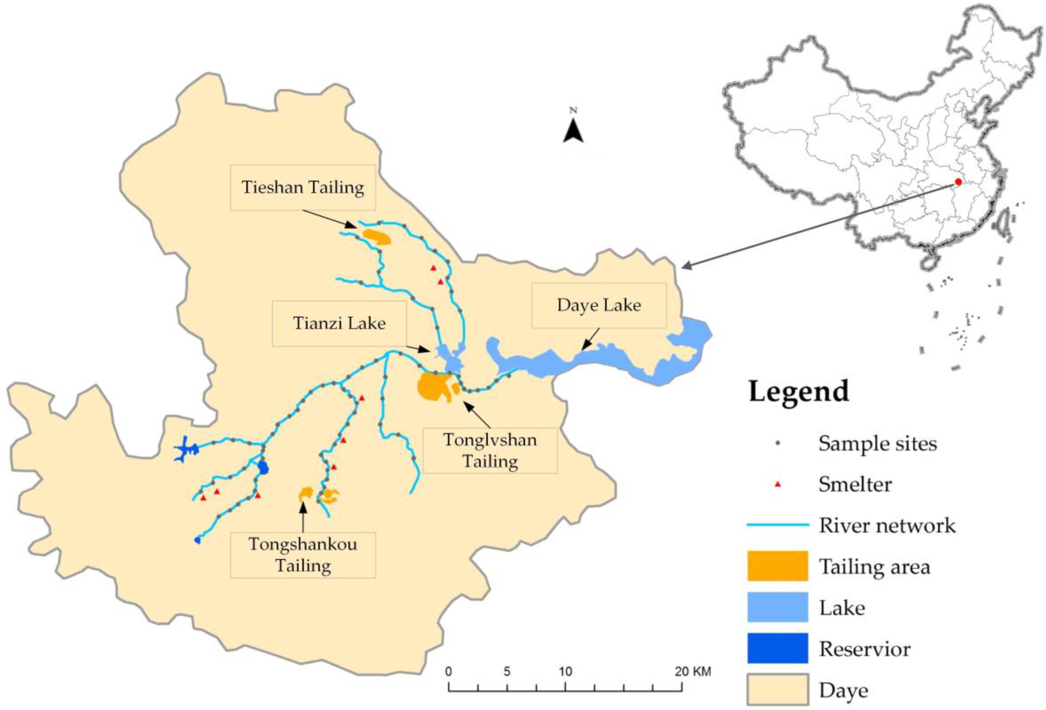
Daye (29°40′–30°15′N, 114°31′–115°20′E) is a county-level city located in the east of Hubei province, China (Figure 1), which has a subtropical monsoon climate, with an annual average temperature and rainfall of 16.9 °C and 1385.8 mm, respectively. A total of 73 sediment samples were randomly collected alongside the river network of Daye in May 2013 (Spring), with all of the sites having collected surface sediment (0–15 cm). The samples have four types of sediment, including sandy silt, sandy mud, silt sand, and gravelly sand. The geograpchical coodinates of sample sites were recorded by a handheld global position system (GPS) and the positioning error is less than 10 m. Approximately 1 kg sediment was collected as samples and was cold-stored in a plastic bag while being transported to a laboratory for chemical analysis. In the laboratory, all of the sediment samples were air dried, ground, screened through a sieve of 2 mm mesh size, and then digested by HCL-HNO3-HF-HCLO4, using the Chinese national standard method (GB/T17140) [28]. The concentrations of copper (Cu) and lead (Pb) were analyzed by atomic absorption spectrophotometer (SPSIC4510, Shanghai, China).
2.2. Network Inverse Distance Weighted Interpolation
Suppose a non-directed network , consisting of a set of nodes and a set of links . Let be the observed attribute values at sample points on , expressed by . An unknown value at an arbitrary point on is predicted using known values in a neighborhood of , denoted by . Thus, the unknown value at is predicted as the weighted average of the known attribute values at the points of a neighborhood , and the value at is interpolated as:
and is calculated by
where . is a predetermined positive parameter that decides how the weight decreases as the distance increases, and is the shortest-path distance from to .
There are no definite rules for determining the value of , and we applied the most popular choice of , so that the data are inversely weighted at the squared distance [15]. The neighborhood in this study was specified using the k-th nearest neighborhood, as defined by nearest points from , where k is a predefined parameter [19]. Similarly, the choice of the number of points in is rather subjective and many empirical studies have demonstrated that the values of can be specified between 3 and 9 [19]. Because the sample size was limited, cross validation was applied in this study. The mean absolute error (MAE) and the root mean square error (RMSE) calculated from the measured and interpolated values at each sample site were used to assess the accuracy of predictions:
where is the interpolated value at location , and is the sample size. Small MRE and RMSE values indicate fewer errors.
2.3. Local Indicators of Network-Constrained Clusters Approaches
Considering the fact that the application of planar analysis methods to network-constrained phenomena could lead to improper pattern inferences, an exploratory methodology, namely local indicators of network-constrained clusters (LINCS), was introduced to detect the local-scale clustering of network events [21,31]. Two types of LINCS methods, namely ILINCS and GLINCS, are the network extension of the local Moran’s I and the local Getis-Ord G statistics, respectively [31,32]. To detect the spatial patterns at a much finer spatial resolution than that imposed by a given network, the links are usually divided into shorter segments in LINCS methods [21,31].
The network autocorrelation analysis modifies the spatial weight matrix to reflect the network connectivity between the links. The local Moran’s I statistic aims to assess the spatial autocorrelation between a unit and its neighbors; however, the local G statistic measures the concentration of attributes of a variable around a unit [33]. In the context of local-scale cluster detection in a network space, each link is usually connected to a relatively small number of other links, thus, the randomization assumption is preferred, and statistical inference based on the Monte Carlo simulation is recommended in related studies [21,32,34]. In this study, the local-scale clustering of heavy metal pollution in river sediments was analyzed using the ILINCS method, which incorporates a Monte Carlo simulation to assess the statistical significance of the detected clusters. The GeoDaNet toolbox [35] is applied to calculate the ILINCS in this research.
3. Results and Discussions
3.1. Sample Characteristics
Statistical analyses, including descriptive statistics, histograms, P-P plots (normal probability plots), and Q-Q plots (normal quantile–quantile plots) were applied in this study and implemented using IBM SPSS Statistics 21. Summary statistics for Cu and Pb contents in river sediments are provided in Table 1. In the study area, the concentrations of Cu and Pb were much higher than the average Chinese soil background value [18], and also higher than the suggested local background value (30.7 mg/kg and 26.7 mg/kg), which might have resulted from the distribution of the sample sites. In this study, sample sites were located along the river network, thus, the sediment sample could be easily influenced by floods carrying heavy metal contents.
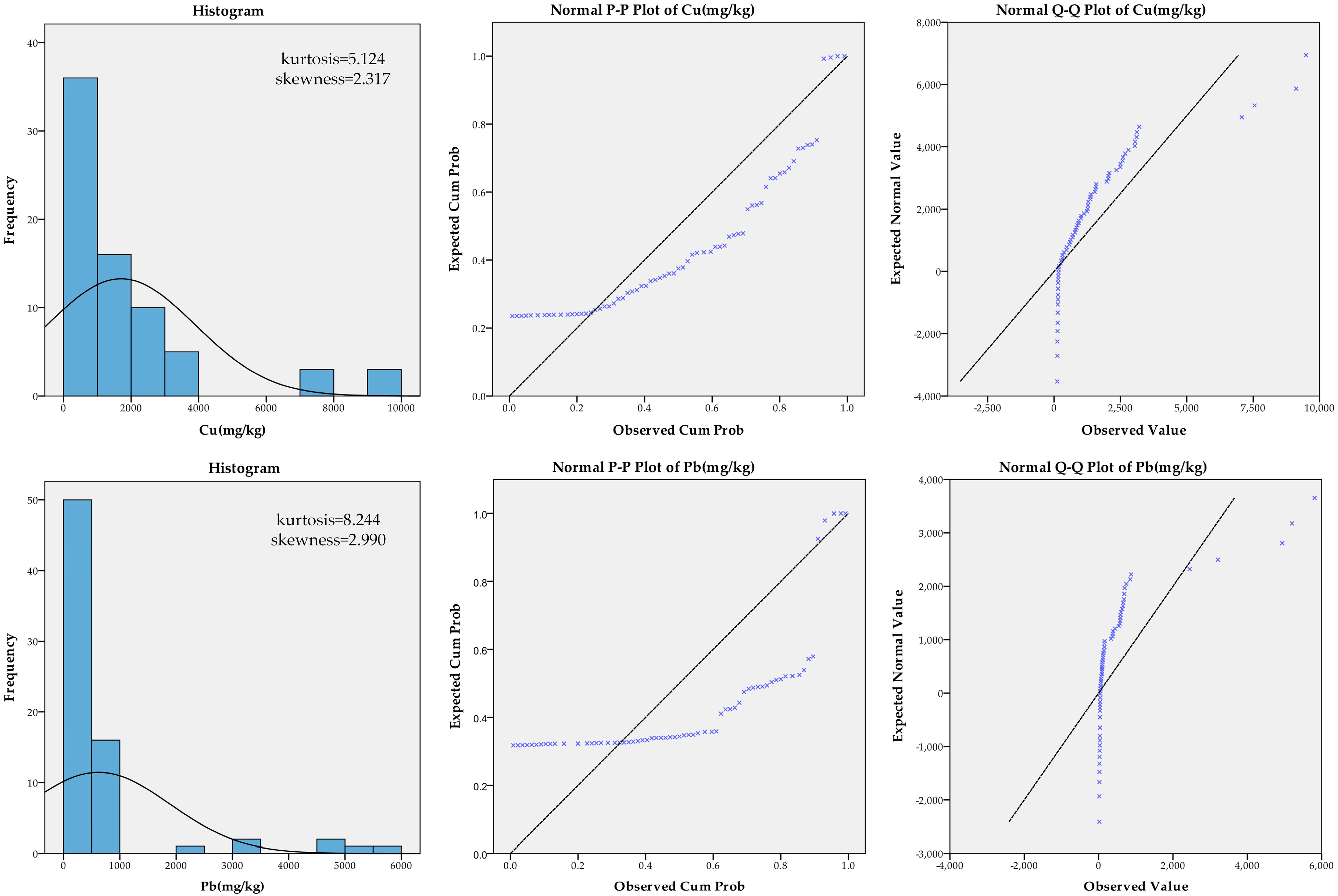
Figure 2 shows the sample data distribution and normality tests results of the total Cu and Pb contents. The histograms suggest that there are some samples with extreme values. The results of the normal P-P plot and Q-Q plot of the total Cu and Pb contents indicate that the sample data of both heavy metal contents are asymmetrical with a peak, and positively skewed. Therefore, the kriging interpolation method was not applied here because of its normality assumption.
3.2. Accuracy of Interpolation Methods
The computation of network inverse distance weighted interpolation (netIDW) was implemented in the ESRI ArcGIS 10.2, using Microsoft Visual C# 2010. The river network was split into shorter segments using a network segmentation algorithm, with a standard length of 100 m [21,34]. In order to analyze the effect of the number of points in the neighborhood on pollution assessment, the parameter in netIDW used 4–7 in this study. In addition, planar interpolation methods, including inverse distance weighting (IDW), local polynomial interpolation (LP), and radial basic functions (RBFs), were evaluated in this study [15]. Specifically, the weight power of IDW used 1–4, the regression coefficient of LP used 1–3, and five radial basis functions, namely completely regularized spline (CRS), inverse multi-quadratic function (IMQ), multi-quadratic function (MQ), spline with tension (ST) and thin-plate spline (TPS), were applied in this study.
The values of the mean absolute error (MAE) and root mean square error (RMSE) are summarized in Table 2. According to the results of cross validation, netIDW is more accurate than other methods, with LP having the biggest estimated error and netIDW5 having the minimum error. NetIDW is sensitive to the number of points in the neighborhood, which controls how the predicted value is weighted by the known attribute values at the points of a neighborhood. A polynomial is usually applied to measure the trends and patterns in the data, rather than as an interpolation method [15]. IDW and RBFs are two widely used interpolation methods that predict a value that is identical to the measured value at a sampled location. IDW creates a surface from measured samples based on the extent of similarity, and the maximum and minimum values in the interpolation surface that can only occur at sample locations. However, based on the degree of smoothing, the RBFs can predict values above the maximum and below the minimum measured values [15,36].
3.3. Spatial Variation of the Cu and Pb Contaminations
In this section, we first measure the spatial distribution of Cu and Pb in river sediments using network inverse distance weighted interpolation, as shown in Figure 3. The results indicate there is an uneven distribution of heavy metal contamination in sediments along the river network. High concentration of Cu and Pb in river sediment is mainly located close to smelters, which is also strongly correlated to the tailing area of Daye. Mining industries that are located at the upper reach of the river have a significant impact on the spatial distribution of the heavy metal contents. The Tieshan tailing area and its adjacent smelters are a major source of Cu and Pb pollution, which may deteriorate the water quality of Tianzi Lake and bring great harm to the water ecological environment of Daye. In addition, the Daye Non-Ferrous Metal Company located in the upper reach of the rivers that flow into Tianzi Lake, could be the major source of Cu and Pb emission [28].
The fact that Cu and Pb have a similar distribution indicates that they might have a similar source in the sediment of this river basin, as shown in a previous study [28]. The spatial distribution characteristics of Cu could be explained by industry waste residue resulting from Cu-Sulfur separation processes, which will stay in the waste residue if not used efficiently. The spatial concentration of Pb is probably associated with the wastewater discharged from the smelting industry. Previous monitoring results have demonstrated that wastewater discharged through smelting industries was abundant in Pb in the study area [37]. However, to identify the real pollution sources of Cu and Pb, further monitoring work on potential pollution sources needs to be implemented in this area.
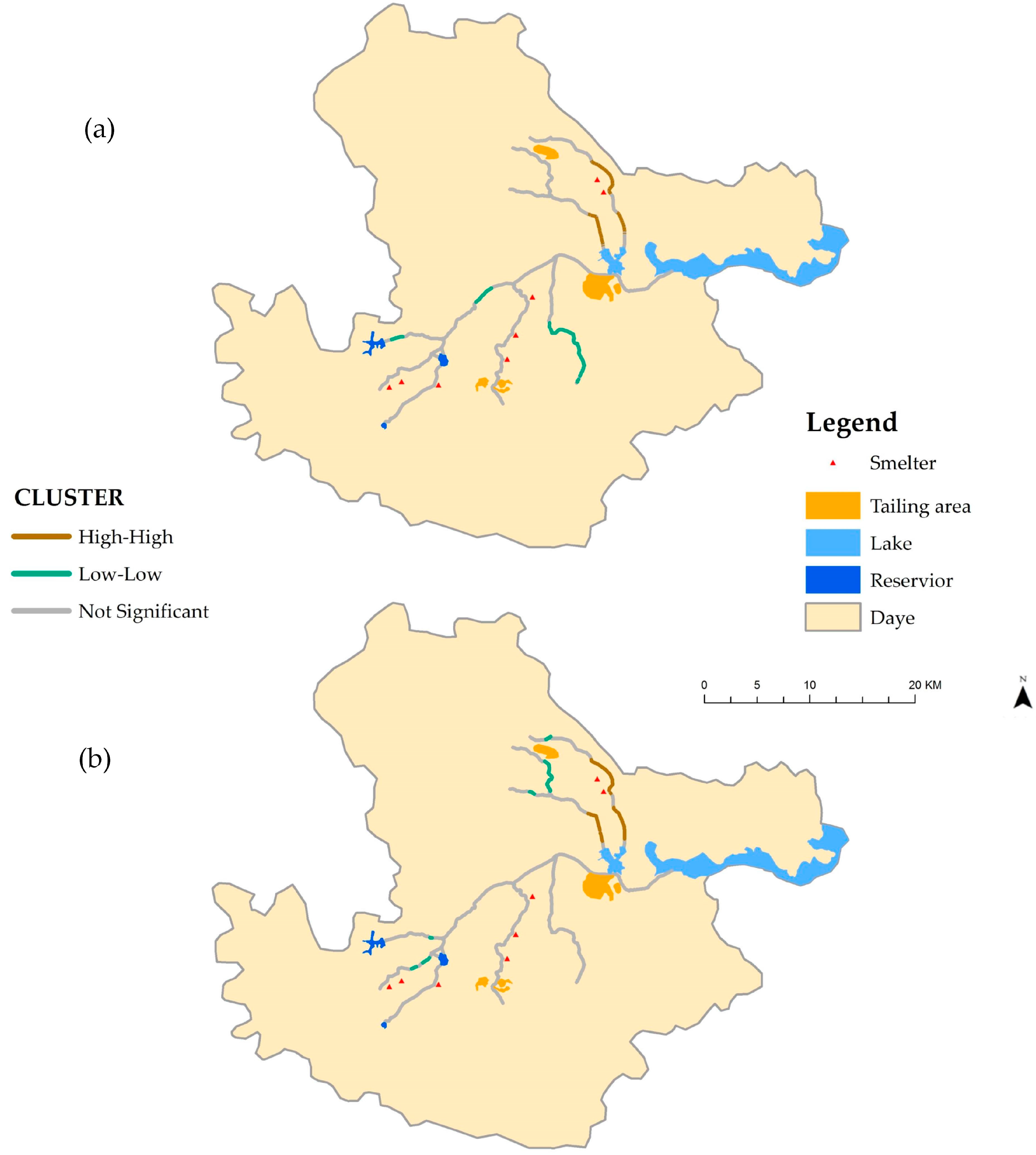
Only visual inspection of spatial concentrations of Cu and Pb contaminations was provided in the results of the network inverse distance interpolation. Therefore, the ILINCS method was then applied in this study, to further explore local spatial patterns of Cu and Pb contaminations in the river sediment. Figure 4 presents the results from the ILINCS method, given 999 conditional permutations and a significance level of 0.01. There is significant network autocorrelation of Cu contaminant in river sediments, and high–high spatial clusters located in the upper reach of the rivers that flow into Tianzi Lake (Figure 4a). These results indicate that smelters may be the main source of Cu emission, in comparison to the Tieshan tailing area. The distribution of high–high spatial clusters of Pb is similar to that of Cu (Figure 4b), which indicates that Cu and Pb could have common pollution sources. In this study, the river network was split into shorter segments, with a standard length of 100 m. However, it is worthwhile searching for the most effective scale of clustering, by examining multiple values of standard length that would reduce potential biases, caused by a presumed cluster size [21].
Effectiveness of pollution evaluation depends on accurate and efficient mapping of heavy metals in river sediment. Generally, a larger number of samples will produce a more accurate map. However, due to the cost of sample collection and chemical analysis, sampling on a large scale is usually impractical, and therefore, the sampling design is essential for heavy metal pollution evaluation [15,38]. In this study, sediment samples were randomly collected alongside the river network of Daye. Although random sampling has several limitations, it is the simplest and most fundamental of probability-based sampling design, and is often used as a first step in other sampling processes [38]. Additional sampling in the region with a high concentration of heavy metals should be done to draw further conclusions.
4. Conclusions
This study was aimed at analyzing spatial distribution characteristics of Cu and Pb contamination in river sediments of Daye, using network spatial analysis methods. The results showed that Cu and Pb contents were unevenly distributed in river sediments, and that the network inverse distance interpolation method was more accurate in assessment, than planar interpolation methods with smaller MAE and RMSE. The ILINCS method was then applied to analyze local spatial patterns of Cu and Pb pollution in river sediments. The results showed that there is significant high-high network autocorrelation in the study region, which is useful in determining sources of pollution in the contaminated areas, as well as in the pollution assessment of Daye.
There are several factors that affect soil pollution mapping, including the number of soil samples, the distance between sampling locations, and the choice of interpolation method [39]. The results of spatial interpolation demonstrate that all of the interpolation techniques have an influence on the pollution area estimation. Even with the same type of interpolation method, the results varied with the parameters of the method. The objective of the interpolations was to estimate the spatial concentrations of heavy metal contents as accurately as possible. In order to minimize the estimated error of global mean, spatial interpolation methods tend to smooth out the original data, which probably contributes towards the high pollution risk area being underestimated, and the clean area overestimated [15]. Therefore, the pollution area estimated by interpolation methods should be further investigated.
This study was conducted in Daye, which was regarded as a ‘resources-exhausting city’ by the Chinese government in 2008. Mining and smelting operations in this region are significant causes of heavy metal contamination in the environment. The findings of this study can be used as an indicator in pollution evaluation, and can assist decision makers to identify the pollution sources for heavy metals. However, there are two main problems that need to be addressed in further research. First, although network inverse distance weighted interpolation outperformed planar interpolation methods, identifying a reach as contaminated should not merely be based on the result of interpolation results. It is suggested that the spatial distribution of heavy metal contents is largely influenced by the natural environment and human activities [2], which should be considered in subsequent analysis. In order to acquire a more reliable pollution assessment, additional sampling at the uncertainty region is necessary. Second, because soil pollution usually has similar pollution sources, the joint distribution of heavy metal contents should be investigated further, to explore the spatial association of heavy metal contaminations. The two problems will be considered together for more comprehensive and detailed results.
Acknowledgments
The research is jointly supported by the National Natural Science Foundation of China (No. 41601407) and the Open Fund of Key Laboratory of Urban Land Resources Monitoring and Simulation, Ministry of Land and Resources (No. KF-2016-02-011).
Author Contributions
Zhensheng Wang designed the approach and conceived the experiments; Zhensheng Wang and Ke Nie wrote most of the manuscript.
Conflicts of Interest
The authors declare no conflict of interest.
References
- Wilson, B.; Pyatt, F.B. Heavy metal dispersion, persistance, and bioccumulation around an ancient copper mine situated in Anglesey, UK. Ecotoxicol. Environ. Saf. 2007, 66, 224–231. [Google Scholar] [CrossRef] [PubMed]
- Huang, J.; Li, F.; Zeng, G.; Liu, W.; Huang, X.; Xiao, Z.; Wu, H.; Gu, Y.; Li, X.; He, X. Integrating hierarchical bioavailability and population distribution into potential eco-risk assessment of heavy metals in road dust: A case study in Xiandao District, Changsha city, China. Sci. Total Environ. 2016, 541, 969–976. [Google Scholar] [CrossRef] [PubMed]
- Khan, S.; Cao, Q.; Zheng, Y.M.; Huang, Y.Z.; Zhu, Y.G. Health risks of heavy metals in contaminated soils and food crops irrigated with wastewater in Beijing, China. Environ. Pollut. 2008, 152, 686–692. [Google Scholar] [CrossRef] [PubMed]
- Zheng, N.; Liu, J.; Wang, Q.; Liang, Z. Health risk assessment of heavy metal exposure to street dust in the zinc smelting district, Northeast of China. Sci. Total Environ. 2010, 408, 726–733. [Google Scholar] [CrossRef] [PubMed]
- Li, Y.; Li, H.; Liu, Z.; Miao, C. Spatial Assessment of Cancer Incidences and the Risks of Industrial Wastewater Emission in China. Sustainability 2016, 8, 480. [Google Scholar] [CrossRef]
- Dong, J.; Yang, Q.; Sun, L.; Zeng, Q.; Liu, S.; Pan, J.; Liu, X. Assessing the concentration and potential dietary risk of heavy metals in vegetables at a Pb/Zn mine site, China. Environ. Earth Sci. 2011, 64, 1317–1321. [Google Scholar] [CrossRef]
- Peters, J.L.; Perlstein, T.S.; Perry, M.J.; McNeely, E.; Weuve, J. Cadmium exposure in association with history of stroke and heart failure. Environ. Res. 2010, 110, 199–206. [Google Scholar] [CrossRef] [PubMed]
- Li, F.; Zhang, J.; Jiang, W.; Liu, C.; Zhang, Z.; Zhang, C.; Zeng, G. Spatial health risk assessment and hierarchical risk management for mercury in soils from a typical contaminated site, China. Environ. Geochem. Health 2016, 1–12. [Google Scholar] [CrossRef] [PubMed]
- Wang, Q.; Cui, Y.; Liu, X. Instances of soil and crop heavy metal contamination in China. Soil Sediment Contam. 2001, 10, 497–510. [Google Scholar]
- Li, Z.; Ma, Z.; van der Kuijp, T.J.; Yuan, Z.; Huang, L. A review of soil heavy metal pollution from mines in China: Pollution and health risk assessment. Sci. Total Environ. 2014, 468–469, 843–853. [Google Scholar] [CrossRef] [PubMed]
- Hu, H.; Jin, Q.; Kavan, P. A Study of Heavy Metal Pollution in China: Current Status, Pollution-Control Policies and Countermeasures. Sustainability 2014, 6, 5820–5838. [Google Scholar] [CrossRef]
- Tang, W.; Shan, B.; Zhang, H.; Zhang, W.; Zhao, Y.; Ding, Y.; Rong, N.; Zhu, X. Heavy Metal Contamination in the Surface Sediments of Representative Limnetic Ecosystems in Eastern China. Sci. Rep. 2014, 4, 7152. [Google Scholar] [CrossRef] [PubMed]
- Liang, J.; Liu, J.; Yuan, X.; Zeng, G.; Lai, X.; Li, X.; Wu, H.; Yuan, Y.; Li, F. Spatial and temporal variation of heavy metal risk and source in sediments of Dongting Lake wetland, mid-south China. J. Environ. Sci. Health A 2015, 50, 100–108. [Google Scholar] [CrossRef] [PubMed]
- Li, F.; Huang, J.; Zeng, G.; Yuan, X.; Li, X.; Liang, J.; Wang, X.; Tang, X.; Bai, B. Spatial risk assessment and sources identification of heavy metals in surface sediments from the Dongting Lake, Middle China. J. Geochem. Explor. 2013, 132, 75–83. [Google Scholar] [CrossRef]
- Xie, Y.; Chen, T.; Lei, M.; Yang, J.; Guo, Q.; Song, B.; Zhou, X. Spatial distribution of soil heavy metal pollution estimated by different interpolation methods: Accuracy and uncertainty analysis. Chemosphere 2011, 82, 468–476. [Google Scholar] [CrossRef] [PubMed]
- Fan, J.; Wang, Y.; Zhou, Z.; You, N.; Meng, J. Dynamic Ecological Risk Assessment and Management of Land Use in the Middle Reaches of the Heihe River Based on Landscape Patterns and Spatial Statistics. Sustainability 2016, 8, 536. [Google Scholar] [CrossRef]
- Her, J.; Park, S.; Lee, J.S. The Effects of Bus Ridership on Airborne Particulate Matter (PM10) Concentrations. Sustainability 2016, 8, 636. [Google Scholar] [CrossRef]
- Chen, Y.; Liu, Y.; Liu, Y.; Lin, A.; Kong, X.; Liu, D.; Li, X.; Zhang, Y.; Gao, Y.; Wang, D. Mapping of Cu and Pb Contaminations in Soil Using Combined Geochemistry, Topography, and Remote Sensing: A Case Study in the Le’an River Floodplain, China. Int. J. Environ. Res. Public Health. 2012, 9, 1874–1886. [Google Scholar] [CrossRef] [PubMed]
- Okabe, A.; Sugihara, K. Spatial Analysis along Networks: Statistical and Computational Methods; John Wiley & Sons: Hoboken, NJ, USA, 2012. [Google Scholar]
- Wang, Z.; Du, Q.; Liang, S.; Nie, K.; Lin, D.; Chen, Y.; Li, J. Analysis of the Spatial Variation of Hospitalization Admissions for Hypertension Disease in Shenzhen, China. Int. J. Environ. Res. Public Health 2014, 11, 713–733. [Google Scholar] [CrossRef] [PubMed]
- Wang, Z.; Yue, Y.; Li, Q.; Nie, K.; Yu, C. Analysis of the Spatial Variation of Network-Constrained Phenomena Represented by a Link Attribute Using a Hierarchical Bayesian Model. ISPRS Int. J. Geo-Inf. 2017, 2, 44. [Google Scholar] [CrossRef]
- Illian, J.; Penttinen, A.; Stoyan, H.; Stoyan, D. Statistical Analysis and Modelling of Spatial Point Patterns; John Wiley & Sons: Hoboken, NJ, USA, 2008. [Google Scholar]
- Haining, R.P. Spatial Data analysis: Theory and Practice; Cambridge University Press: Cambridge, UK, 2003. [Google Scholar]
- Fu, J.; Zhao, C.; Luo, Y.; Liu, C.; Kyzas, G.Z.; Luo, Y.; Zhao, D.; An, S.; Zhu, H. Heavy metals in surface sediments of the Jialu River, China: Their relations to environmental factors. J. Hazard. Mater. 2014, 270, 102–109. [Google Scholar] [CrossRef] [PubMed]
- Kimbrough, S.; Baldauf, R.W.; Hagler, G.S.W.; Shores, R.C.; Mitchell, W.; Whitaker, D.A.; Croghan, C.W.; Vallero, D.A. Long-term continuous measurement of near-road air pollution in Las Vegas: Seasonal variability in traffic emissions impact on local air quality. Air Qual. Atmos. Hlth. 2013, 6, 295–305. [Google Scholar] [CrossRef]
- Nourani, V.; Ejlali, R.G.; Alami, M.T. Spatiotemporal Groundwater Level Forecasting in Coastal Aquifers by Hybrid Artificial Neural Network-Geostatistics Model: A Case Study. Environ. Eng. Sci. 2011, 28, 217–228. [Google Scholar] [CrossRef]
- Okabe, A.; Satoh, T.; Sugihara, K. A kernel density estimation method for networks, its computational method and a GIS-based tool. Int. J. Geogr. Inf. Sci. 2009, 23, 7–32. [Google Scholar] [CrossRef]
- Zhang, J.; Li, Z.H.; Chen, J.; Wang, M.; Tao, R.; Liu, D. Assessment of heavy metal contamination status in sediments and identification of pollution source in Daye Lake, Central China. Environ. Earth Sci. 2014, 72, 1279–1288. [Google Scholar] [CrossRef]
- Deng, H.; Ye, Z.H.; Wong, M.H. Accumulation of lead, zinc, copper and cadmium by 12 wetland plant species thriving in metal-contaminated sites in China. Environ. Pollut. 2004, 132, 29–40. [Google Scholar] [CrossRef] [PubMed]
- Zhang, X.; Hu, M.; Zhao, Y.; Zhao, B. A Survey of Heavy Metals Pollution in Daye Tieshan Area. Enuivon. Sci. Technol. 2005, 28, 40–43. [Google Scholar]
- Yamada, I.; Thill, J. Local indicators of network-constrained clusters in spatial patterns represented by a link attribute. Ann. Assoc. Am. Geogr. 2010, 100, 269–285. [Google Scholar] [CrossRef]
- Anselin, L. Local Indicators of Spatial Association—LISA. Geogr. Anal. 1995, 27, 93–115. [Google Scholar] [CrossRef]
- Getis, A.; Ord, J.K. The Analysis of Spatial Association by Use of Distance Statistics. Geogr. Anal. 1992, 24, 189–206. [Google Scholar] [CrossRef]
- Loo, B.P.Y.; Yao, S. The identification of traffic crash hot zones under the link-attribute and event-based approaches in a network-constrained environment. Comput. Environ. Urban Syst. 2013, 41, 249–261. [Google Scholar] [CrossRef]
- Rey, S.J.; Anselin, L.; Pahle, R.; Kang, X.; Stephens, P. Parallel optimal choropleth map classification in PySAL. Int. J. Geogr. Inf. Sci. 2013, 27, 1023–1039. [Google Scholar] [CrossRef]
- Erdogan, S. A comparision of interpolation methods for producing digital elevation models at the field scale. Earth Surf. Proc. Land. 2009, 34, 366–376. [Google Scholar] [CrossRef]
- Ling, Q.; Yan, S.; Bao, Z. The environmental pollution character and its ecological effect of a large scale smelter. China Environ. Sci. 2006, 26, 603–608. [Google Scholar] [CrossRef]
- Guidance on Choosing a Sampling Design for Environmental Data Collection. Available online: https://www.epa.gov/sites/production/files/2015-06/documents/g5s-final.pdf (accessed on 1 June 2017).
- Kravchenko, A.N. Influence of spatial structure on accuracy of interpolation methods. Soil Sci. Soc. Am. J. 2003, 67, 1564–1571. [Google Scholar] [CrossRef]
Figure 1.
The study area and location of the sample sites.

Figure 2.
Data distribution and normality test results of total Cu and Pb content.

Figure 3.
Spatial distribution of heavy metal contents in river sediments of Daye using network inverse distance weighted interpolation 5 (netIDW5): (a) Cu; (b) Pb.
Figure 3.
Spatial distribution of heavy metal contents in river sediments of Daye using network inverse distance weighted interpolation 5 (netIDW5): (a) Cu; (b) Pb.

Figure 4.
Distribution of spatial clusters of heavy metal contents in river sediments of Daye using ILINCS: (a) Cu; (b) Pb.
Figure 4.
Distribution of spatial clusters of heavy metal contents in river sediments of Daye using ILINCS: (a) Cu; (b) Pb.


Table 1.
Characteristics of Cu and Pb contents in the river sediment sample set (n = 73).
| Heavy Metal Content | Min | Max | Mean | Median | Standard Deviation | Background Value |
|---|---|---|---|---|---|---|
| Cu (mg/kg) | 121.00 | 9490.00 | 1705.92 | 1007.00 | 2195.42 | 20.7 1 |
| Pb (mg/kg) | 18.50 | 5810.00 | 621.15 | 109.00 | 1270.96 | 23.5 1 |
1 Base value of Hubei Province.
Table 2.
The interpolation accuracy of different methods.
| Methods | Mean Absolute Error (MAE) | Root Mean Squared Error (RMSE) | ||
|---|---|---|---|---|
| Cu | Pb | Cu | Pb | |
| netIDW4 | 4.099 | 1.360 | 7.432 | 3.583 |
| netIDW5 | 3.251 | 1.066 | 5.993 | 2.882 |
| netIDW6 | 3.616 | 1.213 | 6.676 | 3.283 |
| netIDW7 | 3.580 | 1.116 | 6.543 | 2.044 |
| IDW1 | 131.107 | 50.370 | 171.801 | 78.105 |
| IDW2 | 7.415 | 3.410 | 15.946 | 6.903 |
| IDW3 | 7.318 | 3.509 | 16.672 | 9.532 |
| IDW4 | 7.530 | 3.610 | 17.747 | 8.636 |
| LP1 | 554.623 | 263.887 | 913.455 | 479.400 |
| LP2 | 465.478 | 205.400 | 825.466 | 444.118 |
| LP3 | 305.627 | 136.610 | 598.253 | 332.665 |
| RBF-CRS | 23.405 | 8.102 | 37.788 | 12.566 |
| RBF-IMQ | 24.315 | 8.339 | 38.999 | 12.752 |
| RBF-MQ | 22.719 | 8.030 | 37.000 | 13.300 |
| RBF-ST | 18.594 | 6.450 | 28.288 | 9.902 |
| RBF-TPS | 24.320 | 8.505 | 35.192 | 12.580 |
© 2017 by the authors. Licensee MDPI, Basel, Switzerland. This article is an open access article distributed under the terms and conditions of the Creative Commons Attribution (CC BY) license (http://creativecommons.org/licenses/by/4.0/).
Share and Cite
MDPI and ACS Style
Wang, Z.; Nie, K. Measuring Spatial Distribution Characteristics of Heavy Metal Contaminations in a Network-Constrained Environment: A Case Study in River Network of Daye, China. Sustainability 2017, 9, 986. https://doi.org/10.3390/su9060986
AMA Style
Wang Z, Nie K. Measuring Spatial Distribution Characteristics of Heavy Metal Contaminations in a Network-Constrained Environment: A Case Study in River Network of Daye, China. Sustainability. 2017; 9(6):986. https://doi.org/10.3390/su9060986
Chicago/Turabian StyleWang, Zhensheng, and Ke Nie. 2017. "Measuring Spatial Distribution Characteristics of Heavy Metal Contaminations in a Network-Constrained Environment: A Case Study in River Network of Daye, China" Sustainability 9, no. 6: 986. https://doi.org/10.3390/su9060986
Note that from the first issue of 2016, this journal uses article numbers instead of page numbers. See further details here.