Evaluating the Scale Effect of Soil Erosion Using Landscape Pattern Metrics and Information Entropy: A Case Study in the Danjiangkou Reservoir Area, China

Abstract

The regular patterns of soil erosion tend to change at different scales of observation, affecting the mechanism of soil erosion and its evolution characteristics. This phenomenon has essential scientific significance for the rational allocation of land resources and for studies on sustainable ecosystems. As an important agricultural area in China, Danjiangkou reservoir is threatened by severe soil erosion. In this study, we selected four kinds of landscape pattern metrics, including patch density, fractal dimension, Shannon diversity index, and connectivity, to analyze soil erosion intensity in the Danjiangkou reservoir area at different scales based on landscape ecological principles. In addition, we determine the optimum research scale of the experimental area by calculating the information entropy value of soil patches at different scales. The findings suggest that: (1) the landscape pattern of soil erosion in the experimental area is obviously scale-dependent, and the responses to scale differ from index to index; (2) as the scale of observation increases, the fragmentation of soil patches is weakened, the stability of different landscape components is enhanced, and the soil becomes less vulnerable to erosion; and (3) based on information entropy theory, 60 m is confirmed to be the optimum scale of this study.

1. Introduction

As a core subject of soil and water conservation research in sustainable ecosystems, soil erosion is affected by various natural and human factors [1,2]. Climate, lithology, soil types, and especially intense land use/cover changes make soil vulnerable to runoff generation and water erosion, leading to the loss of nutrients from the soil, reservoir siltation, and devastating floods [3]. Climatic parameters such as soil moisture, wind, and precipitation are all prone to influence soil erosion. Soil moisture is especially one of the most important factors controlling erosive processes [4], affecting the partitioning of rainfall into infiltration and runoff and consequently influencing soil erosion [5]. Another parameter influencing soil erosion is soil type, as the impact and sensitivity of different soil types to the erosion characteristics arising from land use change are quite different. Purple soil, for instance, was determined to be more sensitive to rainfall intensity in the land-use change from farmland to forest than red soil, black soil, and loess [6]. Moreover, some human impacts have altered land use structures and triggered soil erosion [7]. These land use changes, along with the climate, steep slope, and the fragility of the soil, make the study region very prone to erosion. How to prevent the soil erosion and recover the ecosystems through reasonable land use has become a challenging issue.

Furthermore, the results of studies on soil erosion could vary due to the changes in the scales of observation [8]. Scale is a kind of space or time unit used in studies of certain phenomena, which can be generally divided into a time-scale and space-scale [9,10]. Space-scale refers to the resolution of the smallest recognizable unit; that is, the granularity or the cell size, taking a remote sensing (RS) image as an example. The scale of RS images is an essential factor that must be taken into account when analyzing geospatial issues produced from the RS technique [11]. Methods that deal with spatial autocorrelations are common in non-geostatistical studies. For example, Moran’s ‘I’ and Geary’s ‘C’ statistics are used in spatial correlations for the analysis of raster images [12,13]. Meanwhile, methods based on geo-statistical measures of spatial variability are also widely developed. The most effective method is based on computing a set of textural measures of spatial variability (TMSV) using a moving window [14]. However, the choice of an appropriate moving window size is an important and challenging issue when researching scale-related problems in remote sensing, especially in the scale conversion of raster images. The scale analyses in remote sensing have been achieved by many scholars. For instance, Zhang et al. studied the scale effect of remote sensing images using histo-variograms and conducted scale conversion with an aggregation moving window [15]. Lausch et al. tested and evaluated the suitability of hyper-spectral remote-sensing techniques in detecting the predisposition of spruce vegetation to beetle damage on different spatial scales [16]. The spatial scale effect of mapping plastic-mulched farmland (PMF) was elucidated by Hasituya et al. using high-resolution imagery [17].

Process-based models of ecological function are usually parameterized using measurements at a particular plot, which simplifies only a small fraction of the landscape [18]. This limited sampling means that it is difficult to parameterize ecosystem models across space, which hinders our ability to accurately estimate multi-scale landscapes. Landscape pattern is, to some extent, dependent on scale [19], and changes in scale also have certain impacts on the analyses of landscape patterns [20]. Therefore, landscape pattern research emphasizes the spatial heterogeneity of landscape features [21] and the determination of scales to quantify such variability [22]. Morris et al. quantified the particulate organic matter (POM) cover of a certain area and studied the landscape-scale spatial variation in POM supply to the abyssal seafloor [23]. Furthermore, landscape metrics can be used as indicators of the heterogeneity of different landscape components, which have been studied by many researchers. For example, Zhang et al. assessed ecological security characteristics in the Yuan River watershed based on the relationship between landscape patterns and soil erosion [24]. Morelli et al. explored several models using the metrics of landscape heterogeneity and altitude as predictors of bird diversity in different spatial scales [25]. In another study, the spatial heterogeneity among Greek landscapes was investigated by Plexida and others, where they identified appropriate landscape indicators using different extents [26]. However, among all the above-mentioned studies, few have investigated the importance of the spatial-scale heterogeneity and scale effects on soil erosion in a reservoir region, despite some efforts to research forest and hydrological scale effects. Moreover, appropriate approaches to determine the optimum scale for soil erosion studies are also new area to explore. Here, from the perspective of landscape ecology, we propose a study to investigate ‘landscape pattern-soil erosion’ processes by using landscape metrics and explore the scale effect of soil erosion in an important Chinese agricultural reservoir.

Similarly, few if any examples of scaling in landscape ecology consider the inherent loss or change in information among aggregation process across spatial scales, despite the widespread use of information-theoretic approaches in modeling [27,28]. Changes in information depend on how information is quantified, while techniques from information theory can be applied to quantify how information is gained or lost upon increasing or decreasing the spatial scale of observations [29]. In addition to the selection of entropy for quantifying the amount of information, it can be also chosen for studies on time-scale effects combined with wavelet analysis [30]. Here, we investigate approaches from information theory to determine the optimum research spatial-scale for process-based soil erosion studies. Furthermore, under this optimum cell size, we intend to explore the time-scale effect of soil erosion data combined with wavelet analysis in our future study.

Our research design is based on the Danjiangkou reservoir, China. As an important area in terms of agricultural and economic production in Hubei Province of China, the Danjiangkou reservoir has been threatened by soil erosion. Therefore, this reservoir is taken as a typical area to analyze the relationship between soil erosion and landscape patterns under different spatial scales, as well as to explore the inherent law of changes in soil erosion with spatial scales. In this paper, we aim to detect the scale effect of different landscape pattern metrics for ‘landscape pattern-soil erosion’ studies by using geographic information system (GIS) and remote sensing (RS) technologies. In addition, we attempt to propose a new idea to determine the optimum spatial scale of soil erosion in the reservoir area based on approaches from information entropy theory. The remainder of this paper is organized as follows. After the introduction, Section 2 describes the methodology and data used in this study. Section 3 presents and discusses the main results of our analysis. Section 4 provides a conclusion of the paper and points out limitations for future study.

2. Materials and Methods

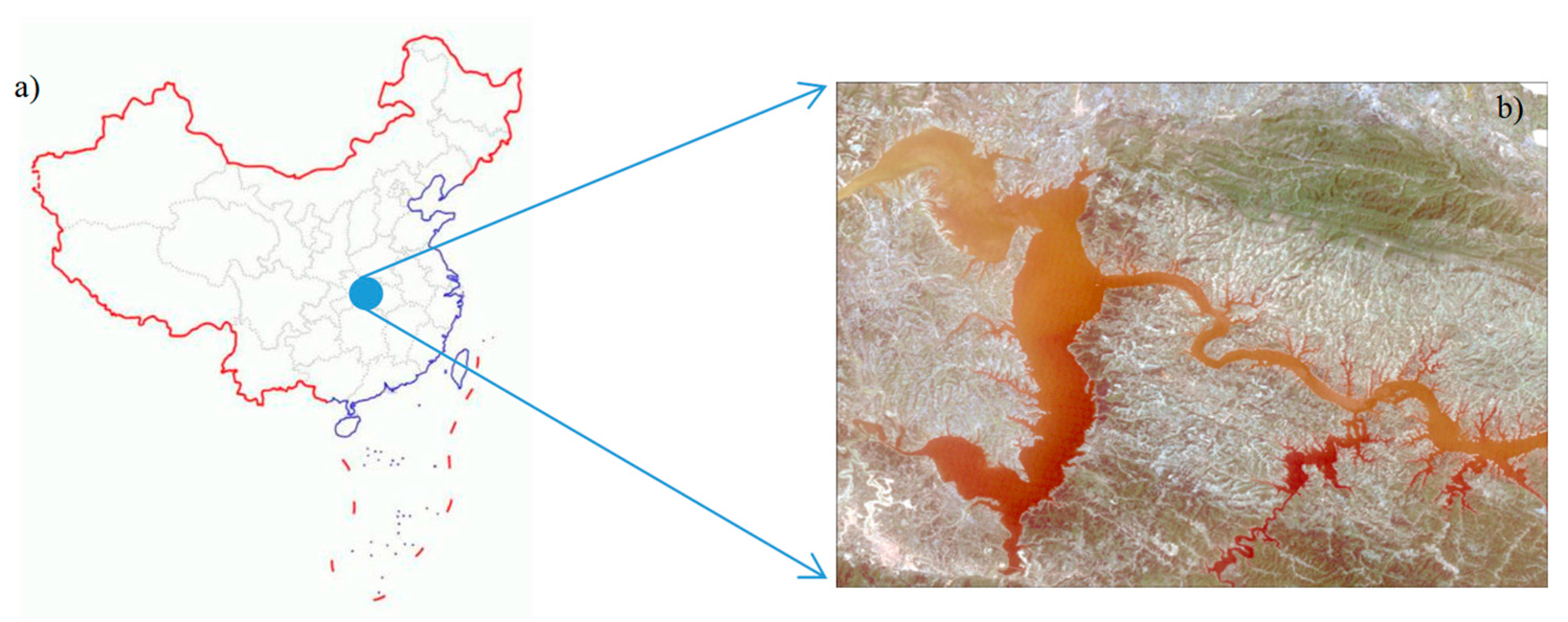
2.1. Study Area and Data

Danjiangkou Reservoir is located in the Yunxian County of Hubei Province, China. The reservoir is bordered by the Danjiangkou city in the east, Xiling of Yunxian County in the west, Wudangtown in the south, and XichuanCounty of Henan Province in the north. The region is situated between 32°36′—33°48′ N and 110°59′—111°49′ E. Figure 1a,b show the relative location and the enlarged image of the area, respectively.

The reservoir’s storage capacity reaches 19 billion m³, which makes it the second-largest artificial reservoir in China. It lies in the transitional zone between the northern subtropics and the warm temperate zone and is affected by the typical monsoon continental semi-humid climate. The region is a relatively independent natural unit, the terrain of which is high in the northwest and low in the southeast. With complex terrain and diverse natural conditions, the reservoir is suitable for the production of vegetation. However, due to poor natural conditions and the impact of human reclamation, the area has experienced different degrees of soil erosion.

The original data used in this study include; Landsat-5 TM images with a resolution of 30 m for the years 2002 and 2009, Digital Elevation Model(DEM) data (with a resolution of 30 m), and other fundamental materials related to soil erosion such as ‘Soil records of Danjiangkou City’.

2.2. Data Processing

In our study, data are processed in GIS and the remote sensing platforms ArcGIS and ENVI. The first data processing step is to transform projection, wherein the administrative data and remote sensing images are projected under a unified projection. Then we use ENVI 5.0 to complete the preprocessing of the remote sensing images of two-year periods, including splicing, cropping, and merging. Through the method of supervised classification, we categorize land use types in the study region into five categories; water, forestland, arable land, construction land, and unused land. Then the land use data is converted into a vector format. The classification of the land-use system is presented in

Table 1. The land use classification system.

First Level Classes	Second Level Classes	Descriptions
Arable land	-	Cultivated lands for crops, including mature cultivated land, newly-cultivated land, reclamation land, shifting cultivated land; crop land in which a crop is a dominant species and land that is used for intercropping such as crop-fruiter; other lands that have been shifted to cultivation temporarily.
	Paddy field	Arable land that has enough water supply and irrigation facilities for the cultivation of paddy rice and other aquatic crops.
	Dry land	Arable land with no water supply and irrigation facilities; arable land that is used for planting dry farming crops with natural precipitation.
Forest land	-	Lands growing trees, including arbor, shrub, bamboo, and for forestry use.
	Forest	Natural or planted forests with tree canopy cover >30%.
	Shrub	Lands covered by trees under 2 m high with canopy cover ≥40%.
	Others	Lands, including sparse woodland and nurseries; lands with the growth of herbs-based land.
Construction land	-	Lands used for settlements, business use, factories, transportation infrastructures, and so on.
	Residential land	Lands used for urban and rural settlements and their ancillary facilities.
	Business land	Lands used for business use, including wholesale and retail land, accommodation land, financial land, and so on.
	Others	Lands used for industrial and mining use, public administration, and public service and lands used for transportation facilities such as airports.
Water	-	Lands covered by natural water bodies or lands with facilities for water reservation.
	Reservoir	Man-made facilities with a total storage capacity more than 10 million cubic meters.
	Lakes and rivers	Lands covered by lakes or rivers, including canals.
Unused land	-	Lands are not utilized or hard to make use of.
	Sandy land	Lands with a surface of sand cover, with no more than 5% vegetation cover.
	Bare land	Bare land with exposed soil or rocks, basically with no vegetation cover.
	Saline land	Lands with saline accumulation and sparse vegetation.
	Undeveloped land	New lands in towns or villages that have not been put into use yet.

.

Vegetation coverage data is extracted from remote sensing images, and slope data is acquired from the DEM. The first step is to calculate the NDVI (normalized differential vegetation index), which is used for constructing vegetation coverage grid data in ArcGIS from the images; the second step is to generate slope grid data, which is derived from the DEM using the ‘slope’ function in the software. Finally, these grid data are converted into vectors to be consistent with the land use data. In this paper, we adopt a method to study soil erosion using a remote sensing monitoring method based on the indicator rules proposed by Zhou in 2005 [31], then overlay the vectors of land use, vegetation coverage, and slope data in order to obtain the soil erosion map.

According to the industrial standard of the People’s Republic of China for the classification and gradation of soil erosion (SL 190-2007), as well as the different combination of topography, geomorphology, land use, and vegetation, the Beijing Municipal Water Resources Bureau formulates a grading system of soil erosion (

Table 2. Grading index of soil erosion intensity.

Vegetation Coverage		Slope (°)
		0~3	3~5	5~8	8~15	15~25	25~35	>35
Forestland	>75%	micro	micro	micro	micro	micro	micro	micro
	60%~75%	micro	micro	mild	mild	mild	moderate	moderate
	45%~60%	micro	micro	mild	mild	moderate	moderate	deep
	30%~45%	micro	micro	mild	moderate	moderate	deep	intensive
	<30%	micro	micro	moderate	moderate	deep	intensive	severe
Arable land and other types	Arable land	micro	mild	mild	moderate	deep	intensive	severe
	Construction land	micro	micro	micro	micro	micro	micro	micro
	Unused land	micro	micro	micro	micro	micro	micro	micro

Note: Intensity classification is judged by land type and erosion factors. For forestland, this is done by using vegetation coverage factor and slope factor; for arable land, by using slope factor directly to determine the erosion intensity; and for other types (water, construction land, and unused land identified as micro-erosion.

).This system divides the erosion intensity into six degrees: (1) micro (no erosion or erosion is not obvious, including forest land with vegetation coverage >75% and lands with slope <5° but not including arable land with a slope of 3~5°); (2) mild (soil erosion is more obvious, including cultivated lands with a slope of 3~8°, land with vegetation coverage of 60~70% and a slope of 5~25°, or land with vegetation coverage of 45~60% and a slope of 5~15°, etc.); (3) moderate (soil erosion is pretty obvious, including cultivated lands with a slope of 8~15°, land with vegetation coverage <30% and a slope of 5~15°, etc.); (4) deep (strong erosion, mainly distributed in mountains with little vegetation, including land with vegetation coverage of 45~60% and a slope >35°, etc.); (5) intensive (intensive erosion, mainly distributed in high hilly slope); (6)and severe (severe erosion, including bare land with sparse vegetation or arable land with a slope higher than 35°).

(3) To test various scale effects of soil erosion, spatial aggregation and scale conversion are processed in ArcGIS to derive a series of data with different spatial resolutions ranging from 30 m to 240 m. We resample the original map (with a resolution of 30 m) and aggregate cells into several larger scale datasets with 30 m increments using an arithmetic average variability weighted (AAVW) algorithm. Then, based on the fractal theory and landscape pattern metrics, we treat the soil erosion unit as a patch from the view of landscape ecology, calculating and comparing the landscape pattern metrics at different spatial scales in order to explore and reveal the inherent law of soil erosion change with scale.

2.3. Calculation of Landscape Pattern Metrics

Landscape pattern metrics can be used to reflect and evaluate the spatial characteristics and the distribution of the landscape [32] such as its fragmentation, complexity, or diversity. In this study, we selected four representative pattern metrics, including Patch Density (PD), Perimeter-Area Fractal Dimension (PAFRAC), Shannon’s Diversity Index (SHDI), and Connectivity (CONNECT).

PD is the number of patches per unit area. The higher the PD, the higher the degree of landscape fragmentation. It reflects the uniform distribution of landscape patches and is conducive to the comparison between landscapes of different sizes.

It can be calculated as follows:

PD = (n/A) × 10000 × 100.

(1)

where A is the area of a certain landscape type (m²), n is the number of patches, and ‘10000 × 100’ represents the number of patches per 100 hectares.

PAFRAC is an index to reveal the relationship between the patch shape and its area, reflecting the complexity of patches and landscape patterns at a given scale of observation [33,34]. Its values are between one and two, with stronger self-similarity in patches when converging towards one, and the shape of patches is also simpler. The expression is shown as follows:

$$\mathrm{PAFRAC}=\frac{\frac{2}{[n_i{{\displaystyle \sum }}_{j=1}^n(\ln p_{ij}\times \ln a_{ij})]-[({{\displaystyle \sum }}_{j=1}^n\ln p_{ij})({{\displaystyle \sum }}_{j=1}^n\ln a_{ij})]}}{(n_i{{\displaystyle \sum }}_{j=1}^n\ln p_{ij}^2)-{({{\displaystyle \sum }}_{j=1}^n\ln p_{ij})}^2}$$

(2)

where n_ij is the number of patches typed as i, a_ij is the jth patch area of patch type i (m²), and p_ij is the jth patch perimeter of patch type i (m).

SHDI reflects the different landscape patterns or the diversity index of a certain kind of landscape pattern at different times. In some landscapes, the richer the land-use, the higher the degree of fragmentation and the higher the value of SHDI. Its calculation formula is:

$$\mathrm{SHDI}=-{\displaystyle \sum }_{j=1}^m(p_i\ln p_i)$$

(3)

where m is the number of landscape types and P_i is the proportion that type i accounts for in all types.

CONNECT is the connection degree of patch-to-patch distance [35,36]. In soil erosion studies, the spatial connectivity of landscape units is very important. For example, the increased connectivity of vegetation patches is conducive to the inhibition of soil erosion [37]. The connect index can be expressed as follows:

$$\mathrm{CONNECT}=({\displaystyle \sum }_{i=1}^m{\displaystyle \sum }_{j=k}^n{c}_{ijk})/({\displaystyle \sum }_{i=1}^m\frac{n_i(n_i-1)}{2})$$

(4)

where c_ijk represents the connection situation between the same type of patches j and k within a given connection threshold (1 for connection and 0 for no connection), n_i is the number of patches for type i, and m is the number of patch types.

3. Results and Discussion

3.1. Scale Effect of Soil Erosion in the Danjiangkou Reservoir Area

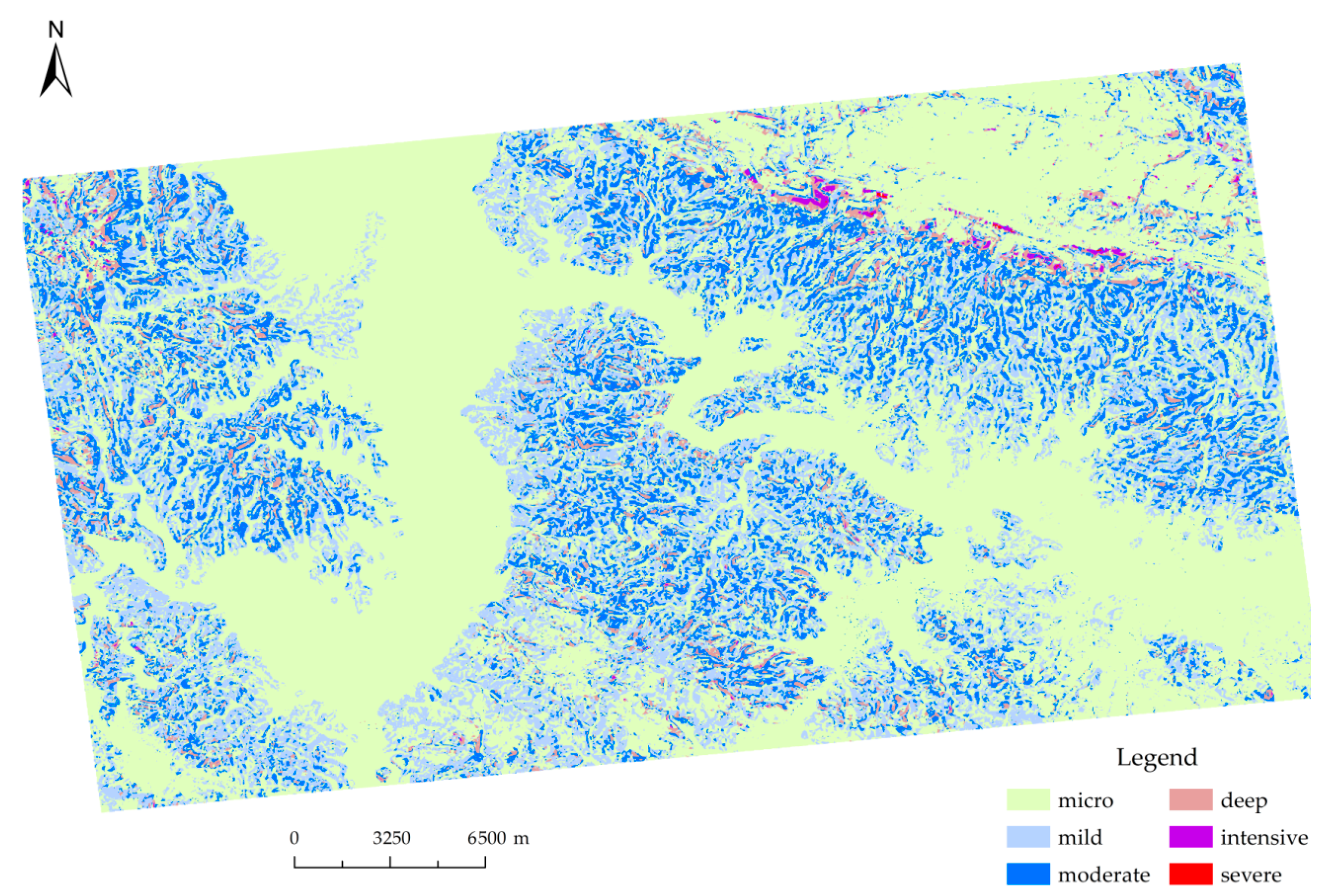
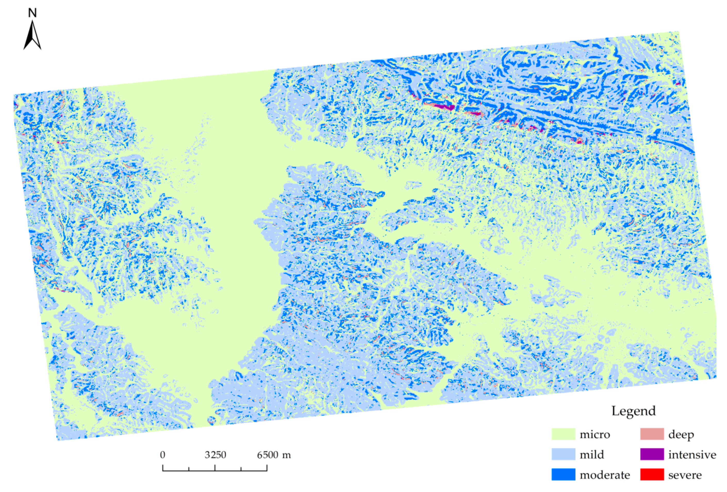
3.1.1. Grading Evaluation of Soil Erosion

Different land-use types, vegetation coverage, topographic gradients, and their combinations correspond to different soil erosion intensity grades. By using the spatial analysis function of ArcGIS, we first overlay the land-use classification map, the vegetation coverage gradation map, and the slope gradation map; then we count the number of cells of soil erosion under each intensity and aggregate the cells with the same erosion degree to obtain the classification tables of soil erosion intensity (

Table 3. Classification of soil erosion intensity in 2002.

Grade Number	Soil Erosion Intensity	Number of Cells (30 m × 30 m)	Percentage
1	micro	194,528	53.88%
2	mild	119,618	33.13%
3	moderate	34,324	9.50%
4	deep	11,555	3.20%
5	intensive	961	0.27%
6	severe	61	0.02%
Total number		361,046	100%

and

Table 4. Classification of soil erosion intensity in 2009.

Grade Number	Soil Erosion Intensity	Number of Cells (30 m × 30 m)	Percentage
1	micro	205,153	60.07%
2	mild	102,243	29.94%
3	moderate	26,874	7.87%
4	deep	6610	1.93%
5	intensive	571	0.17%
6	severe	60	0.02%
Total number		341,512	100%

) and soil erosion intensity grading diagrams (shown in Figure 2 and Figure 3) in Danjiangkou reservoir in the years 2002 and 2009, respectively.

From the charts, we can conclude that the main degrees of soil erosion in the Danjiangkou reservoir area between 2002 and 2009 are micro-erosion and mild-erosion. The total area of erosion decreases to a certain extent in 2009 compared with that in 2002. In the year 2002, micro and mild degrees of soil erosion account for 87.01% of the total erosion area, while moderate erosion and above accounts for 12.99%. However, in 2009, the proportion of micro- and mild-erosion is 90.01% and the percentage of moderate erosion and above is only 9.99%. The results show that, during this period, the intensity of soil erosion in the Danjiangkou reservoir is alleviating, while those areas of more intensive erosion gradually transformed into slighter ones. The total area of micro-erosion increased significantly and the overall level of soil erosion experience a declining trend.

The change in soil erosion can be attributed to natural and human factors. In addition to changes in land use structure, other aspects such as the ‘grain for green project’ and local residents’ promoted awareness of environmental protection, have all contributed to the alleviation of soil erosion. Moreover, the change in agricultural tillage method, wherein the high-load and intensive farming style has been transformed to new eco-friendly one, is also beneficial to lighten the erosion.

3.1.2. Scale Effects of Soil Erosion Patches

Scale effects of soil erosion patches can be explored through analyzing the differences and changing regulations of landscape pattern metrics under different spatial scales [38,39]. Based on the original eroded raster images (with a resolution of 30 m), we generated the soil erosion images at different scales using GIS technology according to an incremental size of 30 m. The maximum raster scale is set as 240 m. Then we calculate and compare the scale response characteristics of each landscape index in two different years. The results are listed in

Table 5. Landscape pattern index values at different scales (in 2002).

Scale(m)	PD	PAFRAC	SHDI	CONNECT
30	61.6811	1.4858	1.3635	0.1614
60	22.9381	1.5813	1.3639	0.1802
90	12.0404	1.6262	1.3643	0.1933
120	7.3581	1.6425	1.3601	0.2122
150	4.9918	1.6561	1.3618	0.2256
180	3.5651	1.6690	1.3640	0.1890
240	2.1285	1.6690	1.3670	0.1633

and

Table 6. Landscape pattern index values at different scales (in 2009).

Scale(m)	PD	PAFRAC	SHDI	CONNECT
30	31.8651	1.4450	1.3111	0.2023
60	13.5211	1.5446	1.3102	0.2407
90	7.2651	1.5918	1.3110	0.2671
120	4.5300	1.5943	1.3113	0.3082
150	3.2065	1.6487	1.3110	0.3334
180	2.3204	1.6458	1.3096	0.2916
240	1.4283	1.6488	1.3097	0.2760

.

It can be noted from the tables that the index values of soil erosion patches have certain responses to the change of scale. The metrics of PD, PAFRAC, and CONNECT are more sensitive to the changes of scale, while the SHDI index has no fluctuation at all. Figure 4 shows the responses of four different metrics to the varying scales.

In terms of these metrics, PD has the largest variation with scale (Figure 4a). With the increase of the scale of observation, the patch density (PD) of the soil erosion unit shows a decreasing trend. The number of patches per unit area of soil is a characterized parameter of landscape fragmentation [40], and the degree of landscape fragmentation is related to natural geographical factors as well as the interference of human economic activities [41]. The higher the soil ecological vulnerability grade is, the less vulnerable soil becomes to erosion and therefore the less intensive the fragmentation of patches is likely to be.

Figure 4b,c show the responses of the PAFRAC and CONNECT metrics due to the increase of scale, respectively, indicating that both of these metrics respond significantly to spatial scales. It is widely acknowledged that the area-perimeter fractal dimension (PAFRAC) is used to describe the complexity of the shape of the patch boundary [31,42]. Therefore, the shape of patches is closely related to their boundary lines, and the shape is supposed to become more complex if the boundary line does. In this study, the growing trend of the PAFRAC index shows that the structure of patches has a moderate scale effect and is projected to suffer higher complexity with the increase of scale.

As for the CONNECT index, the degree of connectivity in landscapes can reflect the diversity, stability, and integrity of different landscape patterns [43]. Therefore, stronger connectivity is also beneficial to the suppression of soil erosion and the maintenance of an ecosystem’s integrity [44]. Figure 4c indicates that the CONNECT index represents scale-dependency to some extent and peaks at the scale of 150 m. This is due to the fact that the stability of different landscape components is enhanced when the scale of the observation is smaller than 150 m, after which the connection of erosion patches is weakened.

Last but not least, the diversity index (SHDI) does not show such significant fluctuations (shown in Figure 4d) as the previous three indices do, which illustrates that the scale effect of the SHDI index is relatively weaker compared to the other metrics, as it responds faintly according to the increase of scale. Therefore, within the selected range of scales, no patch types disappear.

As indicated above, based on the ‘scale-pattern-process’ principle of landscape ecology, we can conclude that, with the increase of scale, the scale effect of PD shows that the fragmentation of soil patches is weakened, and the less vulnerable soil succumbs to erosion. The scale response of PAFRAC indicates that the structure of patches tends to suffer higher complexity; the change of CONNECT suggests that the stability of different landscape components is enhanced when the scale is below 150 m, after which the connection of erosion patches is weakened; and the weak scale effect of the SHDI index illustrates that, within the selected range of scales, nearly no disappearance of patch types occurs.

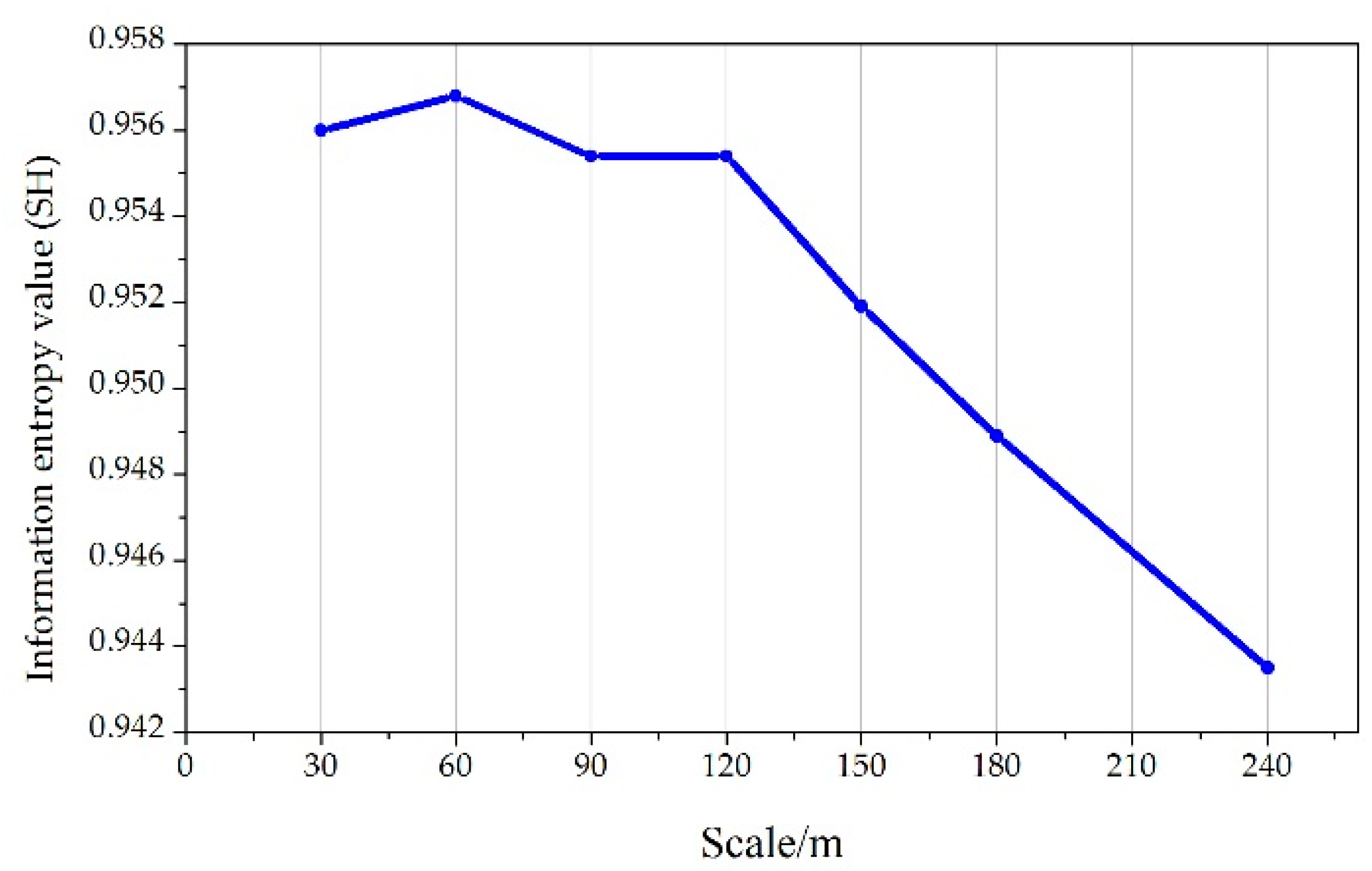
3.2. Optimal Scale Selection of Soil Erosion Based on Information Entropy

At present, many researchers have explored how to determine the best scale to conduct soil erosion research. For example, Lv et al. [45] adopt a method of drawing diagrams of landscape metrics to assign the scale threshold and identify the turning points of landscape metrics to determine the optimal scale. However, this method is significantly affected by subjective factors, which undermine the precision of the results. Other scholars have studied the spatial transfer of soil erosion parameters in agricultural loess areas and found that erosion parameters optimized at smaller scales could be transferred to higher scales without the need for calibration [46]. In this paper, based on the theory of information entropy, we propose a new method to identify the optimal scale of soil erosion research by calculating the information entropy values of erosion patches at different scales, which provides a new way to study scale effects. The basic theoretical framework of this method is as follows.

Land use structure can be analyzed at different scales using entropy [47]. The process of a soil erosion system embodies the proceeding of time and space [48]. In addition to being subject to more or less external constraints, any physical system always has certain internal degrees of freedom, therefore causing the elements within the system to be in different states. If the entropy value is larger on the scale, then the sequence is less self-similar on the scale and the structure is less simple; on the contrary, it is more complex. The maximum entropy occurs when the abundance of the state of things automatically reaches the maximum. In other words, things always strive for (or show) the greatest freedom under constraints, which is the fundamental principle of nature. In most cases, the change of scale will affect the accuracy of the classification of remote sensing images, thereby affecting the amount of information contained in soil erosion patches and the complexity of the erosion system itself. Thus, the assumption is that there must be an optimal scale under which erosion patches contain the most abundant information. In this regard, such scale can be considered the most appropriate.

If the proportion of each erosion category is equal, the information entropy value can reach its maximum value of 1. At this time, the soil erosion system is supposed to be the most complicated, and the information (i.e., diversity) is also the richest in each grid of the patch. However, some types of erosion tend to change to other types over time (for example, areas of moderate erosion and more intensive erosion have transformed into areas of micro and mild erosion over the years in our study area). Then, the order degree of the system will increase and the information entropy value will decrease. The information entropy value will drop to 0 when there is only one type left. Therefore, there must be an extreme information entropy value (closest to 1) when the value of soil erosion changes with scale. The optimal scale selection based on the theory indicated above is calculated as follows.

In information theory, entropy is a measure of the uncertainty of a system. The greater the entropy, the greater the degree of disorder a system contains. Its definition can be expressed as:

$$\mathrm{SH}=-{\displaystyle \sum }_{i=1}^n{P}_i\ln P_i,i=1,2,\dots ,n.$$

(5)

where SH is the information entropy value, n is the number of all events, i represents a random event that occurs in the system, and P_i is the occurrence probability of i. Obviously, ∑P_i=1 satisfies the normalization condition.

For the experimental area, define:

I_k is the study scale (m), $k\in 1,2,\cdots ,7,$ where I_min= 30m, I_max = 240m.

A_i is the eroded area (m²) of different types of soil erosion (classified in Table 1), $i\in 1,2,\cdots ,6$, and the total area of erosion is defined as A.

P_i represents the percentage that each erosion type accounts for in the total area, which can be calculated as follows:

$$P_i=\frac{A_i}{\mathrm{A}}$$

(6)

When A₁ = A₂ = …= A₆, SH_max= 1.

When there is only one A_i and A_i ≠ 0, other erosion types have no area at all; then SH_min = 0.

Thus, there must be I_m; when I_k ≤ I_m, SH increases, and when I_k ≥ I_m, SH decreases. The scale corresponding to the extreme point of the SH value (closest to 1) is supposed to be the optimal scale of soil erosion in this study area.

In this paper, we take the data from the year 2009 as an example. The soil erosion images of Danjiangkou reservoir with different resolutions are graded at each scale (using the method described in Section 3.1.1). Then, the values of A_i and P_i and the information entropy value are calculated at each I_k.

Table 7. Information entropy values of soil erosion under different scales.

Scale (m)	P1	P2	P3	P4	P5	P6	SH
30	0.6007	0.2994	0.0787	0.0193	0.0017	0.0002	0.9560
60	0.5686	0.3407	0.0725	0.0166	0.0015	0.0001	0.9568
90	0.5518	0.3615	0.0701	0.0152	0.0013	0.0001	0.9554
120	0.5391	0.3766	0.0683	0.0146	0.0013	0.0001	0.9554
150	0.5357	0.3823	0.0666	0.0139	0.0014	0.0001	0.9519
180	0.5313	0.3883	0.0656	0.0136	0.0011	0.0001	0.9489
240	0.5324	0.3894	0.0641	0.0129	0.0011	0.0001	0.9435

shows the results (where P₁~P₆ is related to the proportion of the areas of micro, mild, moderate, deep, intensive, and severe erosion to the total erosion area). Based on the results in Table 7, we can draw the response of the information entropy value of soil erosion to the change of scale in our study area (Figure 5).

The results show that the local maximum at a scale of 60 m is highlighted in the charts, and there is an apparent decline in SH beyond the scale of 120 m, which indicates an information loss. Thus, we can reasonably assume that the optimal scale threshold in this study is 60–120 m and that the best scale is located in this threshold interval. In the threshold, the value of SH decreases progressively from the scale of 60 m, which would, therefore, highlight continuous information loss with the increase of scale. Thus, we can conclude that 60 m is the optimal scale in our study area.

As a reflection of the state of open systems [49] such as soil erosion systems, the change of entropy can be used not only to explore the optimal scale, but also to indicate the progress of the erosion system. The evolution of soil erosion follows thermodynamic laws of open systems, wherein a local decrease of entropy is possible and free energy is used to build complex structures while global entropy increases. The fluctuations in open systems decrease the entropy, whereas the irreversible processes restore the system to its initial state. Therefore, the entropy in an isolated system will not reduce continuously (according to the Second Law of Thermodynamics) [50]. A part of the entropy decrease is always accompanied by another part of the entropy increase so as to maintain the stability of open systems. As an open system, soil erosion system follows these dynamic laws with no exception. In the scale response analysis of the information entropy value of soil erosion in the Danjiangkou reservoir area, the entropy increases between the scale of 30 and 60 m and reaches its peak at 60 m, before decreasing dramatically with the further increase of scale.

4. Conclusions

In this paper, we use RS and GIS technologies to explore the scale effect of soil erosion in the Danjiangkou reservoir area between 2002 and 2009. We also use landscape pattern metrics to reveal the scale effect and the evolution law of soil erosion at different scales. In addition, we analyze and identify the optimal scale for the soil erosion of this agricultural area based on information entropy theory. The conclusions are as follows:

(1)

The main degrees of soil erosion in the Danjiangkou reservoir area are micro- and mild-erosion. Compared to the level in 2002, the overall degree of erosion has decreased during this period. The micro- and mild-erosion are concentrated in the arable land with a shallow slope and construction land, while the more severe erosion is clustered in the forestland with little vegetation coverage and a steep slope.

(2)

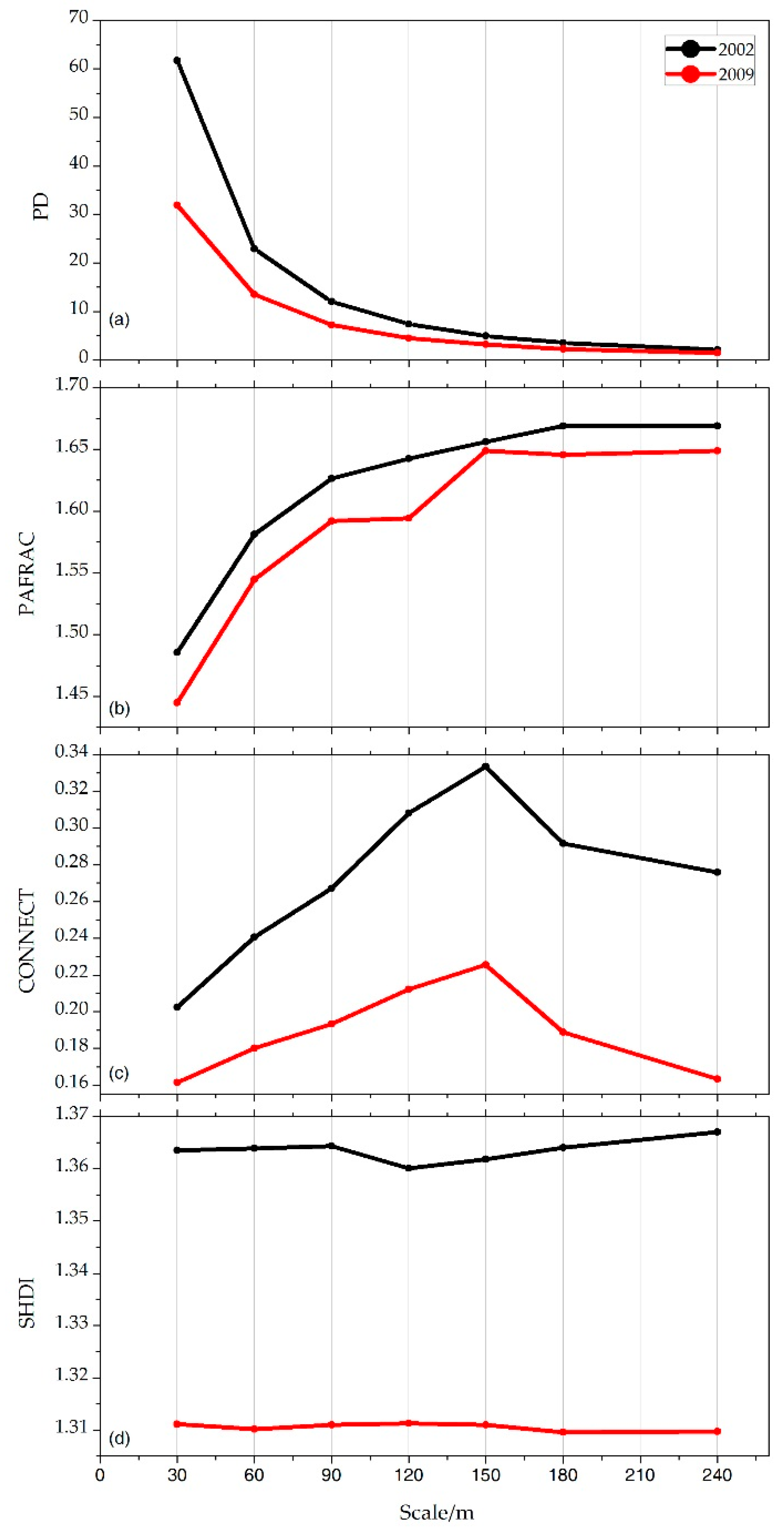
At the holistic level of landscape patterns, the density of soil erosion patches (PD) presents a declining trend with the increase of scale, which demonstrates that the fragmentation of soil patches is weakened and that the less vulnerable soil succumbs to erosion; the area-perimeter fractal dimension (PAFRAC) and the connectivity (CONNECT) fluctuate considerably with scale, showing that the structure of patches tends to suffer higher complexity and that the stability of different landscape components is enhanced when the scale is below 150 m. The response of the diversity index (SHDI) to scale is relatively weak, indicating that nearly no disappearance of patch types occurs within the selected range of scale.

(3)

Information entropy theory is used to reveal the information richness of soil erosion patches. Using this correlation, we identify that the optimal scale threshold in this study is 60–120 m, the value of SH decreases progressively from the scale of 60 m, and there is an obvious decline in SH beyond the scale of 120 m, highlighting an information loss. Thus, the best scale for this reservoir area is supposed to be 60 m.

There are two areas we can improve in the study presented in this paper. First, the landscape pattern metrics we chose in this paper have some limitations if more land use types are taken into consideration. Therefore, it is necessary to include more representative metrics into future research. Secondly, in this paper we investigated approaches from information theory to determine the optimum research spatial-scale for process-based soil erosion studies. Nevertheless, we are also fully aware that time-scale effects of soil erosion can be considered if combined with other mathematical models. Therefore, on top of the optimum spatial cell size method we propose in this paper, we will explore the time-scale effect of soil erosion data using entropy and wavelet analysis in our future work.

References

1. Toor, A.S.; Rana, D.S.; Sur, H.S. Conserve soil and water through grass erosion barriers. Prog. Farming 2003, 39, 16–17. [Google Scholar]
2. Cantón, Y.; Solé-Benet, A.; de Vente, J.; Boix-Fayos, C.; Calvo-Cases, A.; Asensio, C.; Puigdefábregas, J. A review of runoff generation and soil erosion across scales in semiarid south-eastern Spain. J. Arid Environ. 2011, 75, 1254–1261. [Google Scholar] [CrossRef]
3. Sharma, A.; Tiwari, K.N.; Bhadoria, P.B.S. Effect of land use land cover change on soil erosion potential in an agricultural watershed. Environ. Monit. Assess. 2011, 173, 789–801. [Google Scholar] [CrossRef] [PubMed]
4. Wei, L.H.; Zhang, B.; Wang, M.Z. Effects of antecedent soil moisture on runoff and soil erosion in alley cropping systems. Agric. Water Manag. 2007, 94, 54–62. [Google Scholar] [CrossRef]
5. Seeger, M.; Errea, M.P.; Begueria, S. Catchment soil moisture and rainfall characteristics as determinant factors for discharge/suspended sediment hysterestic loops in a small headwater catchment in the Spanish Pyrenees. J. Hydrol. 2004, 288, 299–311. [Google Scholar] [CrossRef]
6. Zhang, S.H.; Li, Y.Q.; Fan, W.W.; Yi, Y.J. Impacts of rainfall, soil type, and land-use change on soil erosion in the Liusha river watershed. J. Hydrol. Eng. 2016, 22, 04016062. [Google Scholar] [CrossRef]
7. McNeill, J.R.; Winiwarter, V. Breaking the sod: Humankind, history and soil. Science 2004, 304, 1627–1629. [Google Scholar] [CrossRef] [PubMed]
8. Zhu, Q.J.; Shuai, Y.M.; Chen, X.; Gan, D.Y.; Yu, F. Soil Erosion Information Entropy: A comprehensive measure index and simulation tool for land surface erodibility. J. Soil Water Conserv. 2002, 16, 50–53. [Google Scholar]
9. Kirkby, M.J.; Imeson, A.C.; Bergkamp, G.; Cammeraat, L.H. Scaling up processes and models from the field plot to the watershed and regional areas. J. Soil Water Conserv. 1996, 51, 391–396. [Google Scholar]
10. Pasquale, B.; Luis, A.S.R.; Brigitta, S. The use of Landsat imagery to assess large-scale forest cover changes in space and time, minimizing false-positive changes. Appl. Geogr. 2013, 41, 147–157. [Google Scholar]
11. Alan, H.S.; Curtis, E.W.; James, A.S. On the nature of models in remote sensing. Remote Sens. Environ. 1986, 20, 121–139. [Google Scholar]
12. Zhang, C.C.; Qin, F.; Wang, Y.X.; Liu, Z.Z.; Chen, Y.S.; Liu, Z.D. Multi-scale quantification of topographic feature using three-dimensional fractal model and its scale effect in watershed: A case of the Two-Tiger Valley of Pisha sandstone area. Res. Soil Water Conserv. 2016, 23, 278–283. [Google Scholar]
13. Panagos, P.; Borrelli, P.; Meusburger, K.; Alewell, C.; Lugato, E.; Montanarella, L. Estimating the soil erosion cover-management factor at the European scale. Land Use Policy 2015, 48, 38–50. [Google Scholar] [CrossRef]
14. Zawadzki, J.; Cieszewski, C.J.; Zasada, M.; Lowe, R.C. Applying geostatistics for investigations of forest ecosystems using remote sensing imagery. Silva Fenn. 2005, 39, 599–617. [Google Scholar] [CrossRef]
15. Zhang, Y.; Jiao, Z.T.; Yang, H.; Li, X.W.; Wang, J.D.; Su, L.H.; Yan, G.J.; Zhao, H.R. Study on scale effect of histogram. Sci. China Ser. D 2002, 32, 307–316. (In Chinese) [Google Scholar]
16. Lausch, A.; Heurich, M.; Gordalla, D.; Dobner, H.J.; Gwillym-Margianto, S.; Salbach, C. Forecasting potential bark beetle outbreaks based on spruce forest vitality using hyperspectral remote-sensing techniques at different scales. For. Ecol. Manag. 2013, 308, 76–89. [Google Scholar] [CrossRef]
17. Hasituya; Chen, Z.X.; Wang, L.M.; Liu, J. Selecting appropriate spatial scale for mapping plastic-mulched farmland with satellite remote sensing imagery. Remote Sens. 2017, 9, 265. [Google Scholar] [CrossRef]
18. Stoy, P.C.; Williams, M.; Spadavecchia, L.; Bell, R.A.; Prieto-Blanco, A.; Evans, J.G.; Van Wijk, M.T. Using information theory to determine optimum pixel size and shape for ecological studies: Aggregating land surface characteristics in Arctic ecosystems. Ecosystems 2009, 12, 574–589. [Google Scholar] [CrossRef]
19. Amy, E.F. A new data aggregation technique to improve landscape metric downscaling. Landsc. Ecol. 2014, 29, 1261–1276. [Google Scholar]
20. Netzel, P.; Stepinski, T.F. Pattern-Based assessment of land cover change on continental scale with application to NLCD 2001–2006. IEEE Trans. Geosci. Remote 2015, 53, 1773–1781. [Google Scholar] [CrossRef]
21. Shi, X.L.; Li, Y.; Deng, R.X. A method for spatial heterogeneity evaluation on landscape pattern of farmland shelterbelt networks: A case study in mid-west of Jilin Province, China. Chin. Geogr. Sci. 2011, 21, 48–56. [Google Scholar] [CrossRef]
22. Li, X.W.; Cao, C.X.; Zhang, Y. A review on scale in remote sensing. J. Remote Sens. 2009, 13, 12–20. (In Chinese) [Google Scholar]
23. Morris, K.J.; Bett, B.J.; Durden, J.M.; Benoist, N.M.; Huvenne, V.A.; Jones, D.O.; Robert, K.; Ichino, M.C.; Wolff, G.A.; Ruhl, H.A. Landscape-scale spatial heterogeneity in phytodetrital cover and megafauna biomass in the abyss links to modest topographic variation. Sci. Rep. 2016, 6, 1–11. [Google Scholar] [CrossRef] [PubMed]
24. Zhang, Z.L.; Liu, S.L.; Dong, S.K. Ecological security assessment of Yuan River watershed based on landscape pattern and soil erosion. Proced. Environ. Sci. 2010, 2, 613–618. [Google Scholar] [CrossRef]
25. Morelli, F.; Pruscini, F.; Santolini, R.; Perna, P.; Benedetti, Y.; Sisti, D. Landscape heterogeneity metrics as indicators of bird diversity: Determining the optimal spatial scales in different landscapes. Ecol. Indic. 2013, 34, 372–379. [Google Scholar] [CrossRef]
26. Plexida, S.G.; Sfougaris, A.I.; Ispikoudis, I.P.; Papanastasis, V.P. Selecting landscape metrics as indicators of spatial heterogeneity—A comparison among Greek landscapes. Int. J. Appl. Earth Obs. 2014, 26, 26–35. [Google Scholar] [CrossRef]
27. Lein, J.K. Toward a remote sensing solution for regional sustainability assessment and monitoring. Sustainability 2014, 6, 2067–2086. [Google Scholar] [CrossRef]
28. Guariglia, E. Entropy and fractal antennas. Entropy 2016, 18, 84. [Google Scholar] [CrossRef]
29. Sharma, A.; Tiwari, K.N.; Bhadoria, P.B. Determining the optimum cell size of digital elevation model for hydrologic application. J. Earth Syst. Sci. 2011, 120, 573–582. [Google Scholar] [CrossRef]
30. Bekiros, S.D. Timescale analysis with an entropy-based shift-invariant discrete wavelet transform. Comput. Econ. 2014, 44, 231–251. [Google Scholar] [CrossRef]
31. Zhou, Y.M. Study on Methods for Soil and Water Conservation Monitoring Small Watershed-Oriented. Ph.D. Thesis, Institute of Remote Sensing Applications; Chinese Academy of Sciences, Beijing, China, 2005. (In Chinese). [Google Scholar]
32. Zhou, Z.X.; Li, J. The correlation analysis on the landscape pattern index and hydrological processes in the Yanhe watershed, China. J. Hydrol. 2015, 524, 417–426. [Google Scholar] [CrossRef]
33. Liu, Y.; Lv, Y.H.; Fu, B.J. Implication and limitation of landscape metrics in delineating relationship between landscape pattern and soil erosion. Acta Ecol. Sin. 2011, 31, 267–275. (In Chinese) [Google Scholar]
34. Guariglia, E. Fractional Derivative of the Riemann Zeta Function. 2015. Available online: https://www.degruyter.com/downloadpdf/books/9783110472097/9783110472097-022/9783110472097-022.pdf (accessed on 16 July 2017).
35. Uezu, A.; Metzger, J.P.; Vielliard, J.M.E. Effects of structural and functional connectivity and patch size on the abundance of seven Atlantic Forest bird species. Biol. Conserv. 2005, 123, 507–519. [Google Scholar] [CrossRef]
36. Wang, J.P.; Yang, L.; Wei, W.; Chen, L.D.; Huang, Z.L. Effects of landscape patterns on soil and water loss in the hilly area of loess plateau in China: Landscape-level and comparison at multiscale. Acta Ecol. Sin. 2011, 31, 5531–5541. [Google Scholar]
37. Michael, W.L.; Paul, A.W.; Maile, C.N. Temporal variability in potential connectivity of Vallisneria Americana in the Chesapeake Bay. Landsc. Ecol. 2016, 31, 2307–2321. [Google Scholar]
38. Wei, W.; Chen, L.D.; Yang, L.; Fu, B.J.; Sun, R.H. Spatial Scale effects of water erosion dynamics: Complexities, variabilities, and uncertainties. Chin. Geogr. Sci. 2012, 22, 127–143. [Google Scholar] [CrossRef]
39. Li, A.N.; Deng, W.; Kong, B.; Lu, X.N.; Feng, W.L.; Lei, G.B.; Bai, J.H. A study on wetland landscape pattern and its change process in Huang-Huai-Hai(3H) area, China. J. Environ. Inf. 2013, 21, 23–34. [Google Scholar] [CrossRef]
40. Janneke, R.W.; Moritz von der, L.; Ingo, K. Seed traits, landscape and environmental parameters as predictors of species occurrence in fragmented urban railway habitats. Basic Appl. Ecol. 2011, 12, 29–37. [Google Scholar]
41. Gao, J.B.; Li, S.C. Detecting spatially non-stationary and scale-dependent relationships between urban landscape fragmentation and related factors using Geographically Weighted Regression. Appl. Geogr. 2011, 31, 292–302. [Google Scholar] [CrossRef]
42. Guariglia, E.; Silvestrov, S. A functional equation for the Riemann zeta fractional derivative. In Proceedings of the AIP Conference Proceedings of ICNPAA 2016 World Congress, American Institute of Physics, La Rochelle, France, 5–8 July 2016; Volume 1798, p. 020063. [Google Scholar] [CrossRef]
43. Marycarol, H.; Bruce, D.; Noah, B. 2010 Joint Meeting of International Study Group for the Multiple Use of Land (ISOMUL) and the Council of Educators in Landscape Architecture (CELA) (review). Landsc. J. 2012, 30, 162–166. [Google Scholar]
44. Marta, A.M.; Santiago, B. Do atmospheric teleconnection patterns influence rainfall erosivity? A study of NAO, MO and WeMO in NE Spain, 1955–2006. J. Hydrol. 2012, 450–451, 168–179. [Google Scholar]
45. Lv, Z.Q.; Wu, Z.F.; Zhang, J.H. Landscape pattern analysis of Guangzhou based on optimization-scale. Geogr. Geo-Inf. Sci. 2007, 23, 89–92. (In Chinese) [Google Scholar]
46. Scherer, U.; Zehe, E. Predicting land use and soil controls on erosion and sediment redistribution in agricultural loess areas: Model development and cross scale verification. Hydrol. Earth Syst. Sci. 2015, 12, 3527–3592. [Google Scholar] [CrossRef]
47. Hu, L.; He, Z.; Liu, J.; Zheng, C. Method for measuring the information content of terrain from digital elevation models. Entropy 2015, 17, 7021–7051. [Google Scholar] [CrossRef]
48. Aucelli, P.P.C.; Massimo, C.; Marta, D.S.; Maurizio, D.M.; Lorenzo, D.; Carmen, M.R.; Francesca, V. Multi-temporal digital photogrammetric analysis for quantitative assessment of soil erosion rates in the Landola catchment of the Upper Orcia Valley(Tuscany, Italy). Land Degrad. Dev. 2016, 27, 1075–1092. [Google Scholar] [CrossRef]
49. Hu, C.Y.; Tang, H.S.; Deng, L.X.; Xue, S.T. The application of an immune clonal selection algorithm based on the information entropy in truss structure multi-objective optimizatio. Appl. Mech. Mater. 2013, 249, 1119–1125. [Google Scholar]
50. Kondepudi, D.; Prigogine, I. Entropy production, fluctuations and small systems. In Modern Thermodynamics: From Heat Engines to Dissipative Structures, 2nd ed.; John Wiley& Sons Ltd.: Chichester, UK, 2014; pp. 323–340. [Google Scholar]
Figure 1. Location of Danjiangkou Reservoir in China: (a) the relative location; and (b) the enlarged remote sensing image of the reservoir.
Sustainability 09 01243 g001
Figure 2. Intensity grading diagram of soil erosion in the reservoir area in 2002.
Sustainability 09 01243 g002
Figure 3. Intensity grading diagram of soil erosion in the reservoir area in 2009.
Sustainability 09 01243 g003
Figure 4. Scale effects of four different metrics at the varying spatial scales. (a) The figure of the patch density index; (b) figure of the perimeter-area fractal dimension index; (c) figure of the connectivity index; and (d) figure of the Shannon’s diversity index.
Sustainability 09 01243 g004
Figure 5. Changes of soil erosion information entropy values at different scales.
Sustainability 09 01243 g005