Application of WEHY-HCM for Modeling Interactive Atmospheric-Hydrologic Processes at Watershed Scale to a Sparsely Gauged Watershed

Abstract
:1. Introduction
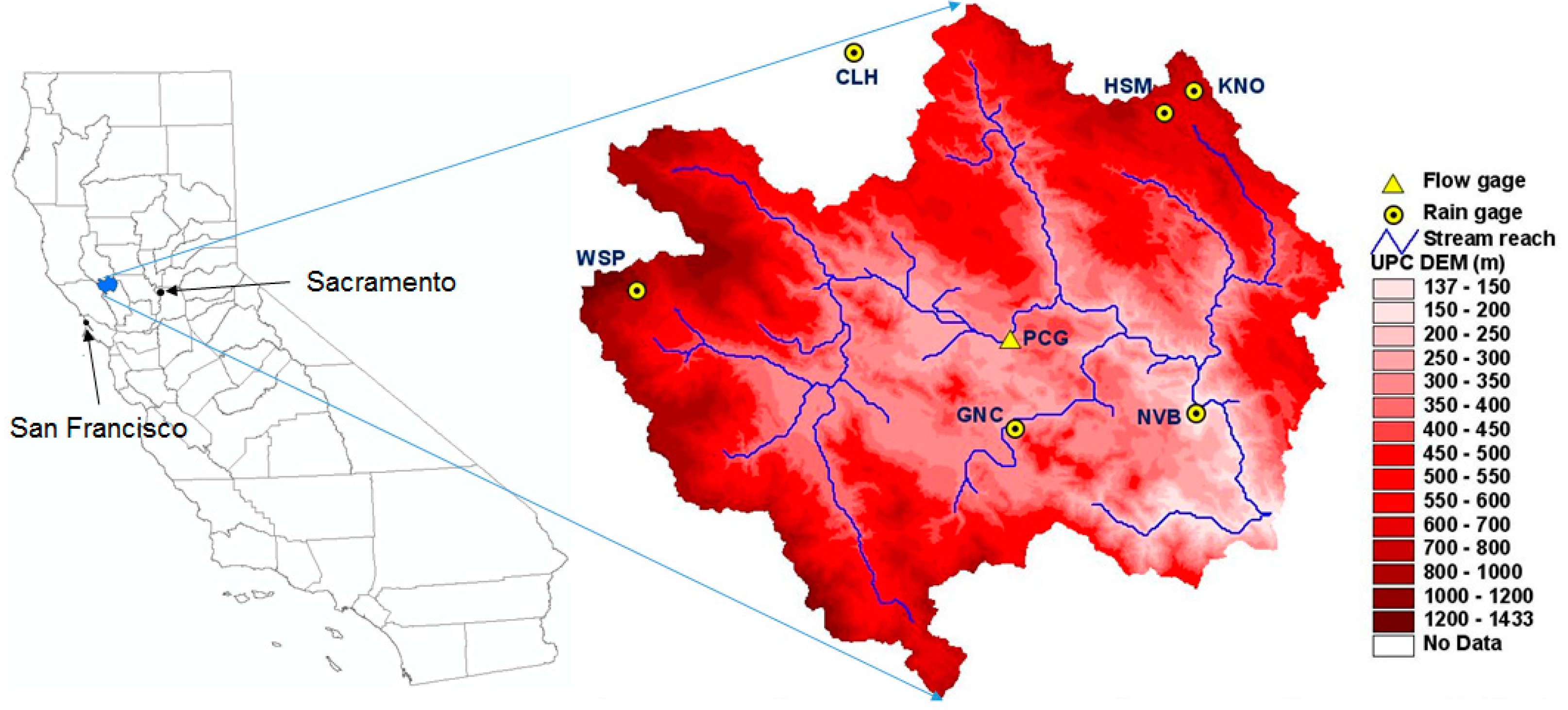
2. Study Area
3. Reconstruction of Historical Atmospheric Conditions
3.1. Methodology for Generating a Reconstructed Atmospheric Data
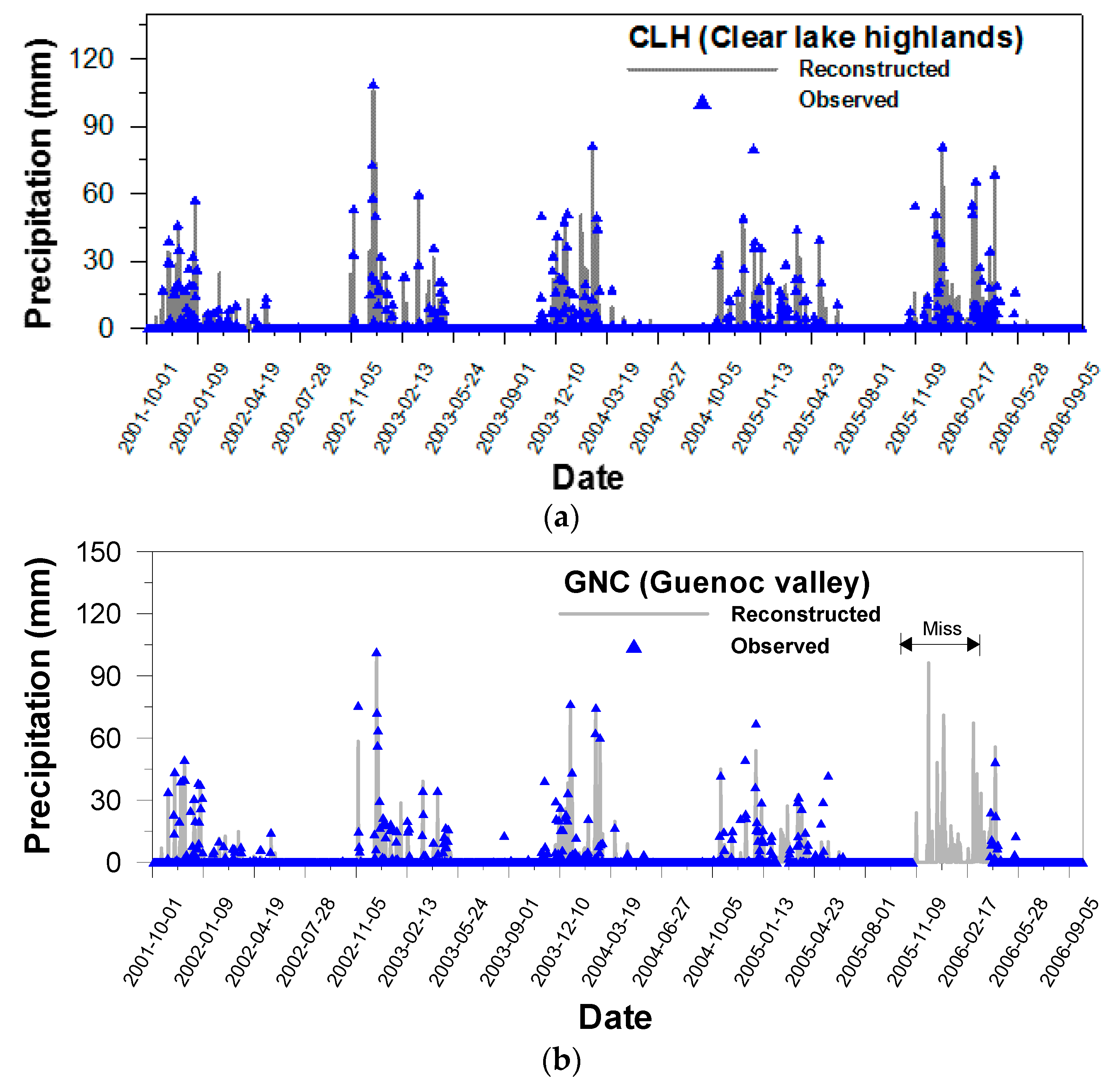
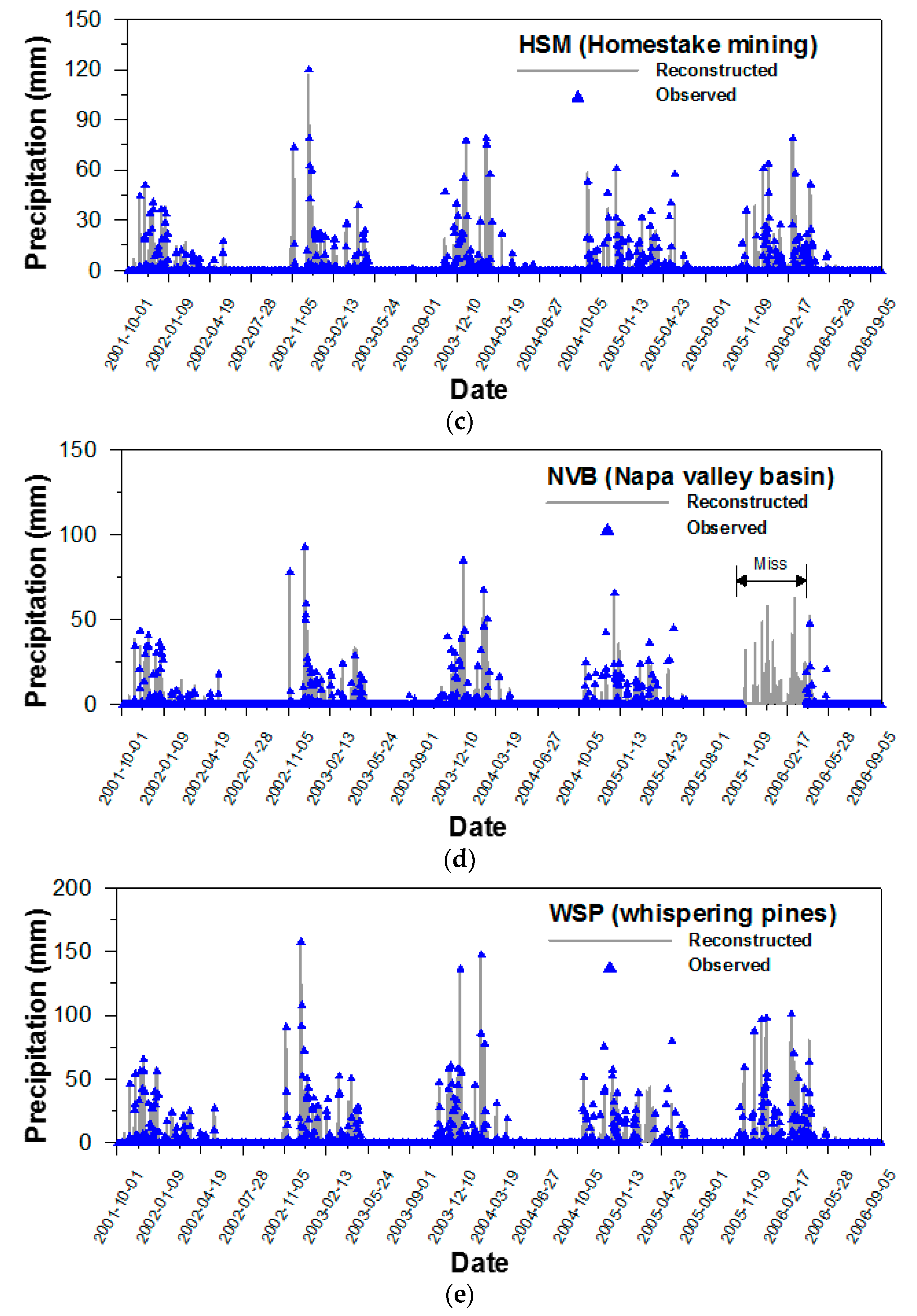
3.2. Bias Correction and Reconstruction of Atmospheric Data
4. Implementation of WEHY Model over Upper Putah Creek Watershed
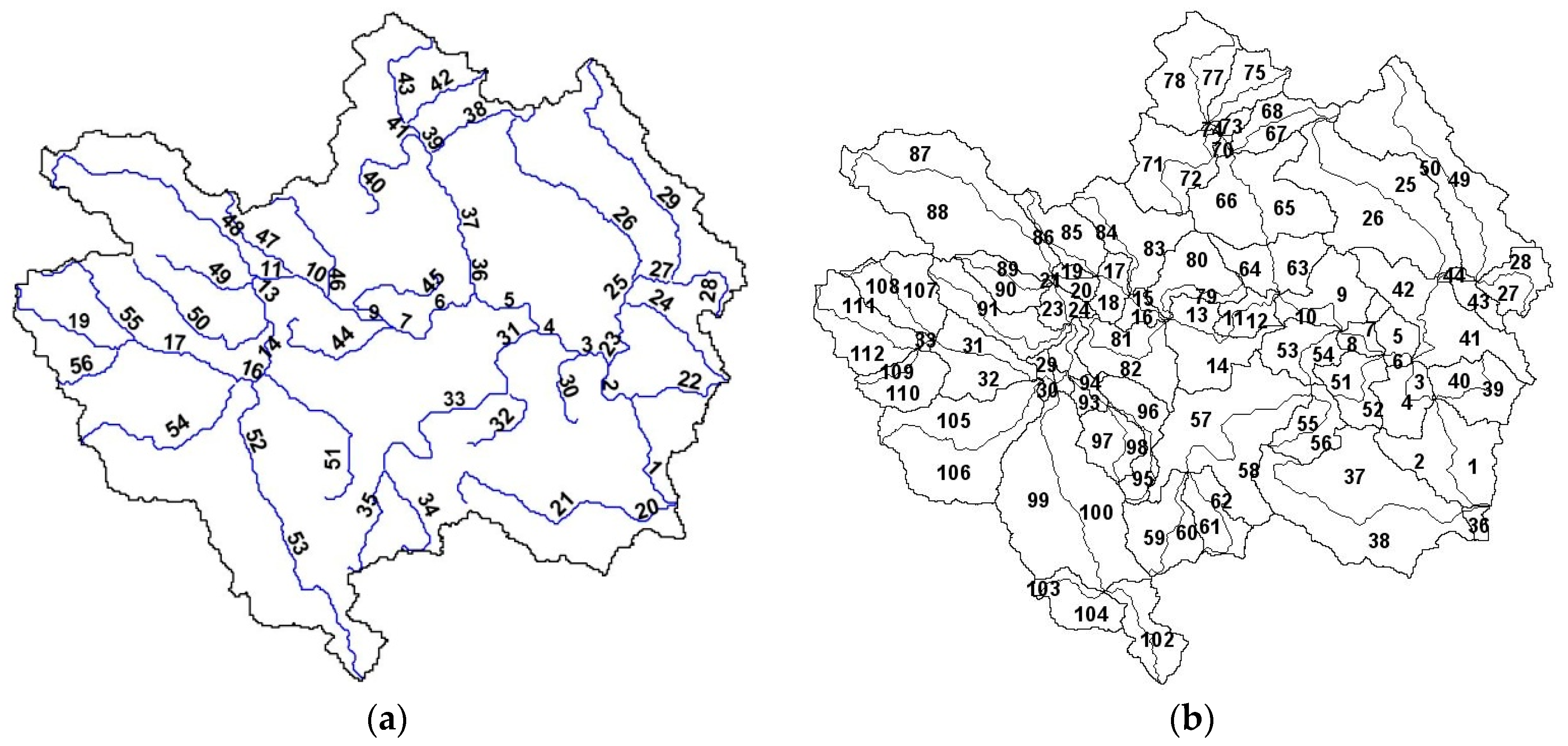
4.1. Delineation of Stream Reaches and Model Computationl Units
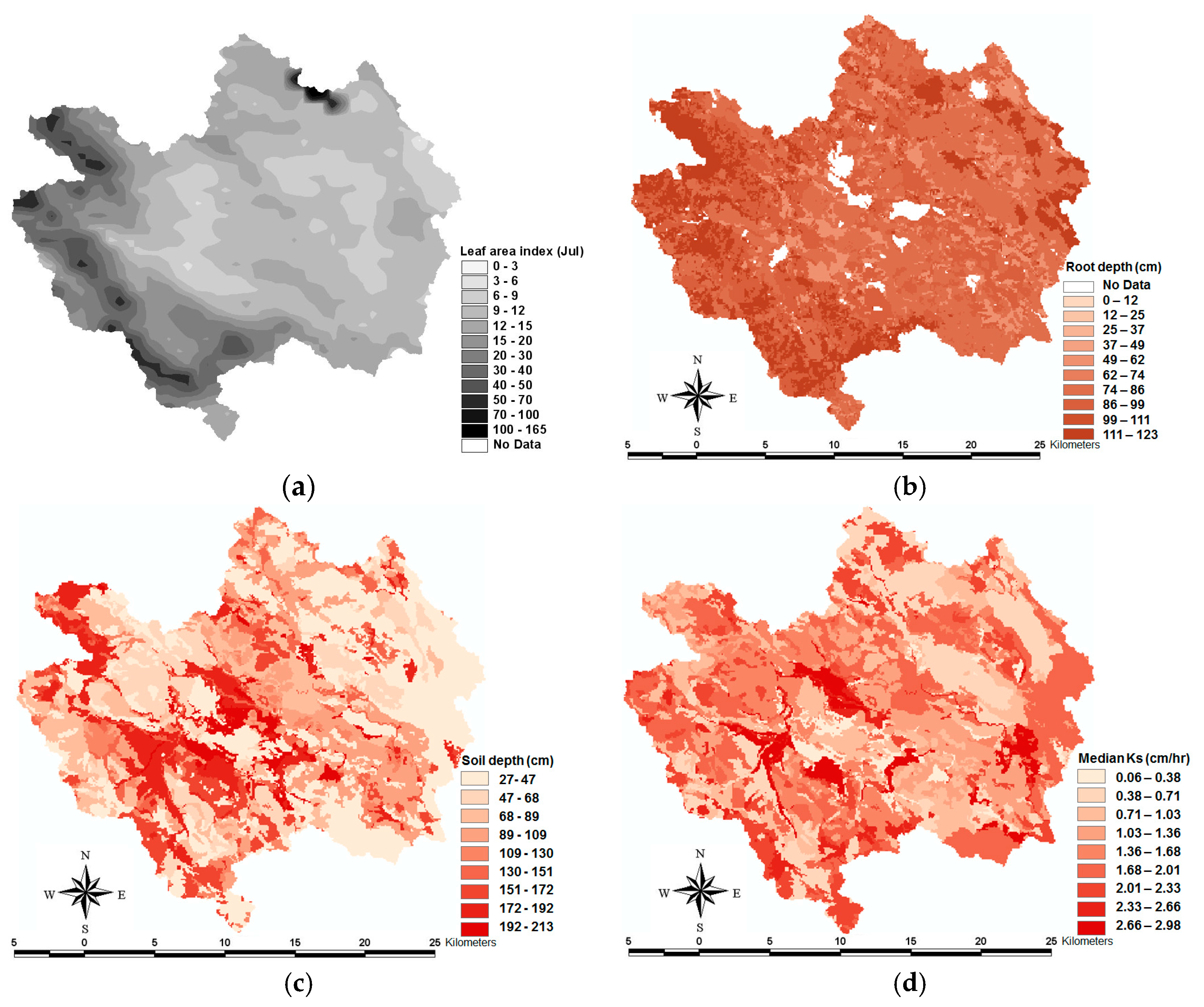
4.2. Estimation of Geommorphologic, Land Surface, and Soil Hydraulic Parameters
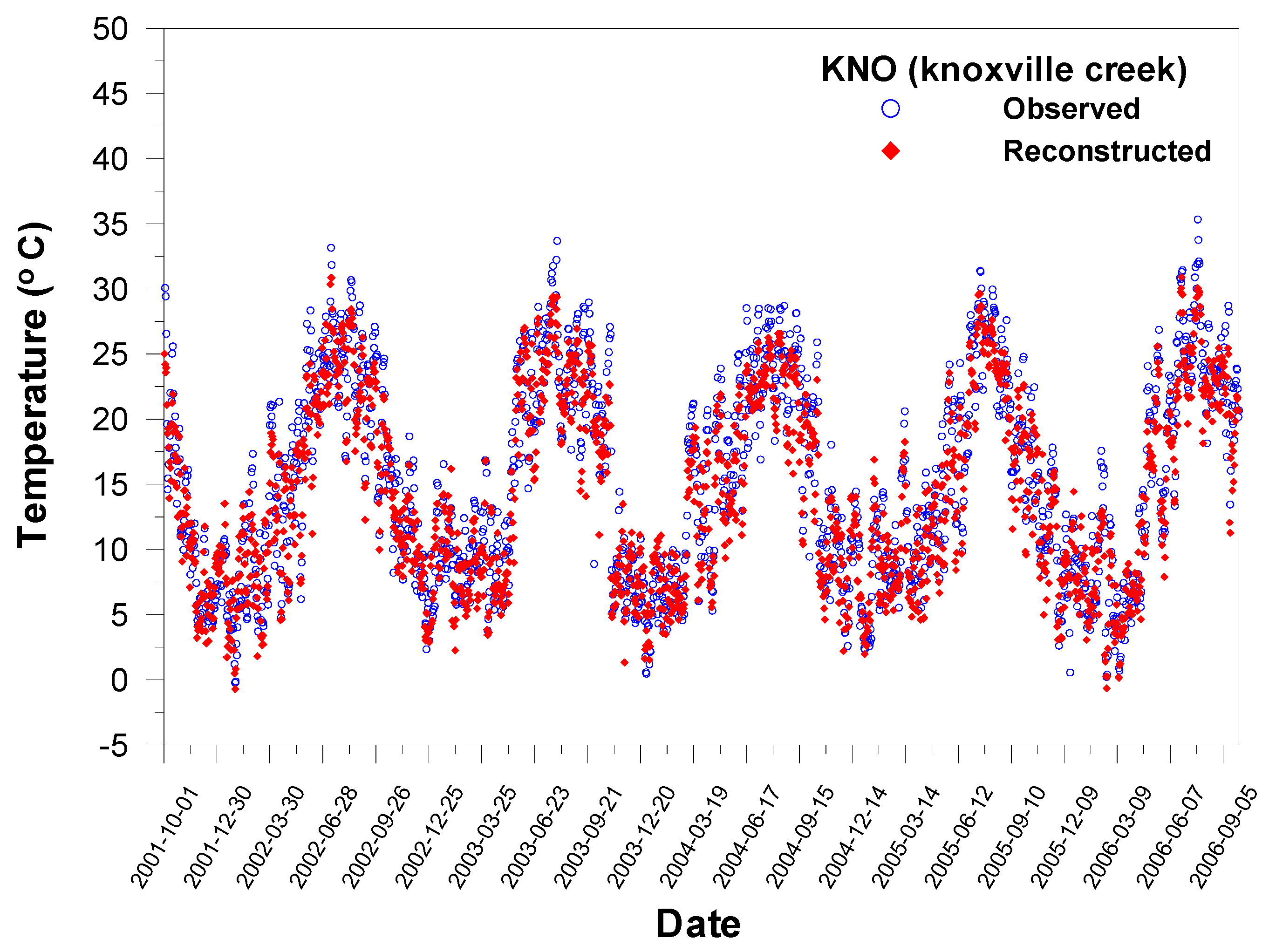
5. Discussion of WEHY-HCM Application Results
6. Conclusions
Acknowledgments
Author Contributions
Conflicts of Interest
References
- Maraun, D.; Wetterhall, F.; Ireson, A.M.; Chandler, R.E.; Kendon, E.J.; Widmann, M.; Brienen, S.; Rust, H.W.; Sauter, T.; Themeßl, M.; et al. Precipitation downscaling under climate change: Recent developments to bridge the gap between dynamical models and the end user. Rev. Geophys. 2010, 48, RG3003. [Google Scholar] [CrossRef]
- Kure, S.; Jang, S.; Ohara, N.; Kavvas, M.L.; Matanga, G.; Nelson, K. Spatial and Temporal Downscaling of Atmospheric Components from GCMs for Historical Reconstructeion and/or for Future Climate Change Study. In Proceedings of the World Environmental and Water Resources Congress 2012, Albuquerque, NM, USA, 20–24 May 2012. [Google Scholar]
- Kavvas, M.L.; Chen, Z.Q.; Dogrul, C.; Yoon, J.Y.; Ohara, N.; Liang, L.; Aksoy, H.; Anderson, M.L.; Yoshitani, J.; Fukami, K.; et al. Watershed Environmental HYdrology (WEHY) Model, based on upscaled conservation equations: Hydrologic module. J. Hydrol. Eng. 2004, 9, 450–464. [Google Scholar] [CrossRef]
- Kampf, S.K.; Burges, S.J. A framework for classifying and comparing distributed hillslope and catchment hydrologic models. Water Resour. Res. 2007, 43, W05423. [Google Scholar] [CrossRef]
- Sayama, T.; McDonnell, J.J. A new time-space accounting scheme to predict stream water residence time and hydrograph source components at the watershed. Water Resour. Res. 2009, 45, W07401. [Google Scholar] [CrossRef]
- Sivapalan, M.; Takeuchi, K.; Franks, S.W.; Gupta, V.K.; Karambiri, H.; Lakshmi, V.; Liang, X.; McDonnell, J.J.; Mendiondo, E.M.; O’Connell, P.E.; et al. IAHS decade on predictions in ungauged basins (PUB), 2003–2012: Shaping an exciting future for the hydrological sciences. Hydrol. Sci. J. 2003, 48, 857–880. [Google Scholar] [CrossRef]
- Cavadias, G.S.; Ouarda, T.B.M.J.; Bobee, B.; Girard, C. A canonical correlation approach to the determination of homogeneous regions for regional flood estimation of ungauged basins. Hydrol. Sci. J. 2001, 46, 499–512. [Google Scholar] [CrossRef]
- Sedaghi, S.H.; Singh, J.K. Derivation of flood hydrographs for un-gauged upstream sub-watersheds using a main outlet hydrograph. J. Hydrol. Eng. 2010, 15, 1059–1069. [Google Scholar] [CrossRef]
- Global Precipitation Measurement (GPM). Available online: https://pmm.nasa.gov/data-access/downloads/gpm (accessed on 10 August 2017).
- TRMM Multi-Satellite Precipitation. Available online: https://pmm.nasa.gov/data-access/downloads/trmm (accessed on 10 August 2017).
- Global Satellite Mapping of Precipitation (GSMaP). Available online: http://sharaku.eorc.jaxa.jp/GSMaP/index.htm (accessed on 10 August 2017).
- Advanced Microwave Scanning Radiometer 2 (AMSR-2). Available online: http://lance.nsstc.nasa.gov/amsr2-science (accessed on 10 August 2017).
- NCEP/EMC U.S. Gridded Precipitation. Available online: http://data.eol.ucar.edu/ (accessed on 10 August 2017).
- Coe, M.T.; Birkett, C.M. Calculation river discharge and prediction of lake height from satellite radar altimetry: Example for the Lake Chad basin. Water Resour. Res. 2004, 40, W10205. [Google Scholar] [CrossRef]
- Bjerklie, D.M.; Moller, D.; Smith, L.C.; Dingman, S.L. Estimating discharge in rivers using remotely sensed hydraulic information. J. Hydrol. 2005, 309, 191–209. [Google Scholar] [CrossRef]
- Sun, W.; Ishidaira, H.; Bastola, S. Estimating discharge by calibrating hydrological model against water surface width measured from satellites in large ungauged basins. Annu. J. Hydraul. Eng. 2009, 53, 49–54. [Google Scholar]
- Sayama, T.; Ozawa, G.; Kawakami, T.; Nabesaka, S.; Fukami, K. Rainfall-runoff-inundation analysis of the 2010 Pakistan flood in the Kabul River basin. Hydrol. Sci. J. 2012, 57, 298–312. [Google Scholar] [CrossRef]
- Kure, S.; Jang, S.; Ohara, N.; Kavvas, M.L.; Chen, Z.Q. WEHY-HCM for modeling interactive atmospheric-hydrologic processes at watershed scale. II: Model application to ungauged and sparsely-gauged watersheds. J. Hydrol. Eng. 2013, 18, 1272–1281. [Google Scholar] [CrossRef]
- Shrivastava, P.K.; Tripathi, M.P.; Das, S.N. Hydrological modeling of a small watershed using satellite data and gis technique. J. Indian Soc. Remote Sens. 2004, 32, 145–157. [Google Scholar] [CrossRef]
- Jang, S.; Kavvas, M.L. Downscaling global climate simulations to regional scales: Statistical downscaling versus dynamical downscaling. J. Hydrol. Eng. 2015, 20, A4014006. [Google Scholar] [CrossRef]
- Kavvas, M.L.; Kure, S.; Ohara, N.; Jang, S.; Chen, Z.Q. WEHY-HCM for modeling interactive atmospheric-hydrologic processes at watershed scale. I: Model description. J. Hydrol. Eng. 2013, 18, 1262–1271. [Google Scholar] [CrossRef]
- Chen, Z.Q.; Kavvas, M.L.; Yoon, J.Y.; Dogrul, E.C.; Fukami, K.; Yoshitani, J.; Matsuura, T. Geomorphologic and soil hydraulic parameters for Watershed Environmental HYdrology (WEHY) Model. J. Hydrol. Eng. 2004, 9, 465–479. [Google Scholar] [CrossRef]
- Chen, Z.Q.; Kavvas, M.L.; Fukami, K.; Yoshitani, J.; Matsuura, T. Watershed Environmental HYdrology (WEHY) Model: Model application. J. Hydrol. Eng. 2004, 9, 480–490. [Google Scholar] [CrossRef]
- Kavvas, M.L.; Yoon, J.; Chen, Z.Q.; Liang, L.; Dogrul, E.C.; Ohara, N.; Aksoy, H.; Anderson, M.L.; Reuter, J.; Hackley, S. Watershed Environmental HYdrology Model: Environmental module and its application to a California watershed. J. Hydrol. Eng. 2006, 11, 261–272. [Google Scholar] [CrossRef]
- Grell, G.; Dudhia, J.; Stauffer, D. A Description of the Fifthgeneration Penn State/NCAR Mesoscale Model (MM5); NCAR Technical Note NCAR/TN-398_STR; National Center for Atmospheric Research: Boulder, CO, USA, 1995. [Google Scholar]
- Dunne, T. Chapter 7: Field studies of hillslope flow processes. In Hillslope Hydrology; Kirkby, M.J., Ed.; Wiley: Chichester, UK, 1978; pp. 227–293. [Google Scholar]
- Horton, R.E. The role of infiltration in the hydrologic cycle. Trans. Am. Geophys. Union 1933, 14, 446–460. [Google Scholar] [CrossRef]
- Horton, R.E. An approach towards a physical interpretation of infiltration capacity. Proc. Soil Sci. Soc. Am. Proc. 1940, 4, 399–417. [Google Scholar]
- Kalnay, E.; Kanamitsu, M.; Kistler, R.; Collins, W.; Deaven, D.; Gandin, L.; Iredell, M.; Saha, S.; White, G.; Woollen, J.; et al. The NCEP/NCAR 40-year reanalysis project. Bull. Am. Meteorol. Soc. 1996, 77, 437–471. [Google Scholar] [CrossRef]
- Anderson, M.L.; Chen, Z.Q.; Kavvas, M.L.; Yoon, J.Y. Reconstructed historical atmospheric data by dynamical downscaling. J. Hydrol. Eng. 2007, 12, 156–162. [Google Scholar] [CrossRef]
- California Data Exchange Center (CDEC). Available online: http://cdec.water.ca.gov/ (accessed on 10 August 2017).
- Amin, M.Z.M.; Shaaban, A.J.; Ercan, A.; Ishida, K.; Kavvas, M.L.; Chen, Z.Q.; Jang, S. Future climate change impact assessment of watershed scale hydrologic processes in Peninsular Malaysia by a regional climate model coupled with a physically-based hydrology model. Sci. Total Environ. 2017, 575, 12–22. [Google Scholar] [CrossRef] [PubMed]
- U.S. Geological Survey (USGS) National Elevation Dataset (NED). Available online: https://lta.cr.usgs.gov/ned (accessed on 10 August 2017).
- California Wildlife Habitat Relationships (CWHR) Multi-Source Land Cover Data. Available online: http://climate.calcommons.org/dataset/multi-source-land-cover-data (accessed on 10 August 2017).
- Asner, G.P.; Scurlock, J.M.O.; Hicke, J.A. Global synthesis of leaf area index observations: Implications for ecological and remote sensing studies. Glob. Ecol. Biogeogr. 2003, 12, 191–205. [Google Scholar] [CrossRef]
- Scurlock, J.M.O.; Asner, G.P.; Gower, S.T. Worldwide Historical Estimates of Leaf Area Index, 1932–2000; ORNL/TM-2001/268; Environmental Science Division, U.S. Department of Energy: Washington, DC, USA, 2001.
- Canadell, J.; Jackson, R.B.; Ehleringer, J.R.; Mooney, H.A.; Sala, O.E.; Schulze, E.D. Maximum rooting depth of vegetation types at the global scale. Oeclogia 1996, 108, 583–595. [Google Scholar] [CrossRef] [PubMed]
- Moderate Resolution Imaging Spectroradiometer (MODIS) Leaf Area Index (LAI). Available online: https://modis.gsfc.nasa.gov/data/dataprod/mod15.php (accessed on 10 August 2017).
- Natural Resources Conservation Service (NRCS) Soil Parameters Were Estimated Using the Soil Survey Geographic (SSURGO) Database. Available online: https://datagateway.nrcs.usda.gov/GDGOrder.aspx (accessed on 10 August 2017).
- Gale, M.R.; Grigal, D.F. Vertical root distribution of northern tree species in relation to successional status. Can. J. For. Res. 1987, 17, 829–834. [Google Scholar] [CrossRef]
- McCuen, R.H.; Rawls, W.J.; Brakensiek, D.L. Statistical analysis of the Brooks-Corey and the Green-Ampt parameters across soil textures. Water Resour. Res. 1981, 2, 1005–1013. [Google Scholar] [CrossRef]
- Yoshitani, J.; Kavvas, M.L.; Chen, Z.Q. Chapter 7: Regional-scale hydroclimate model. In Mathematical Models of Large Watershed Hydrology; Singh, V.P., Frevert, D.K., Eds.; Water Resources Publications, LLC: Littleton, CO, USA, 2002; pp. 237–282. [Google Scholar]
- ASCE Task Committee on Definition of Criteria for Evaluation of Watershed Models. Criteria for evaluation of watershed models. J. Irrig. Drain. Eng. 1993, 119, 429–442. [Google Scholar]
- Martinec, J.; Rango, A. Merits of statistical criteria for the performance of hydrological models. Water Resour. Bull. 1989, 25, 421–432. [Google Scholar] [CrossRef]
- Nash, J.E.; Sutcliffe, J.V. River flow forecasting through conceptual models Part 1—A discussion of principles. J. Hydrol. 1970, 10, 282–290. [Google Scholar] [CrossRef]
- Bingner, R.L.; Murphee, C.E.; Mutchler, C.K. Comparison of sediment yield models on watershed in Mississippi. Trans. ASAE 1989, 32, 529–534. [Google Scholar] [CrossRef]
- Mishra, A.; Kar, S.; Singh, V.P. Determination of runoff and sediment yield from a small watershed in sub-humid subtropics using the HSPF model. Hydrol. Process. 2007, 21, 3035–3045. [Google Scholar] [CrossRef]
- Kavvas, M.L.; Chen, Z.Q.; Tan, L.; Soong, S.-T.; Terakawa, A.; Yoshitani, J.; Fukami, K. A regional-scale land surface parameterization based on areally-averaged hydrological conservation equations. Hydrol. Sci. J. 1998, 43, 611–631. [Google Scholar] [CrossRef]
- Kure, S.; Kavvas, M.L.; Ohara, N.; Jang, S. Upscaling of coupled land surface process modeling for heterogeneous landscapes: Stochastic approach. J. Hydrol. Eng. 2011, 16, 1017–1029. [Google Scholar] [CrossRef]
- Ohara, N.; Kavvas, M.L.; Chen, Z.Q.; Anderson, M.; Liang, L.; Wilcox, J.; Mink, J. Estimation of ET Based on Reconstructed Atmospheric Conditions and Remotely Sensed Information over Last Chance Creek Watershed, Feather River Basin, California. In Proceedings of the World Environmental and Water Resources Congress 2007: Restoring Our Natural Habitat, Tampa, FL, USA, 15–19 May 2007. [Google Scholar]


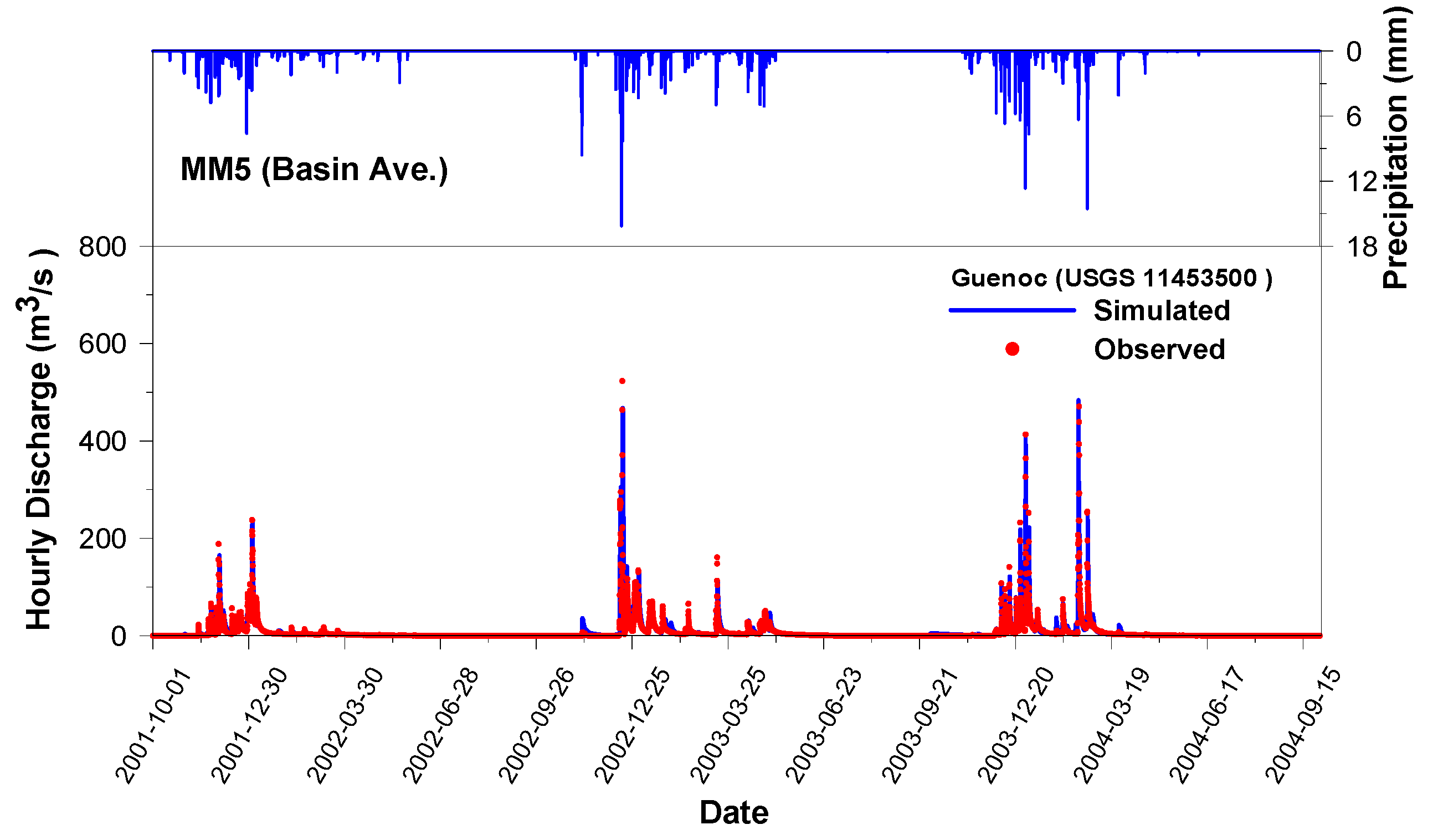
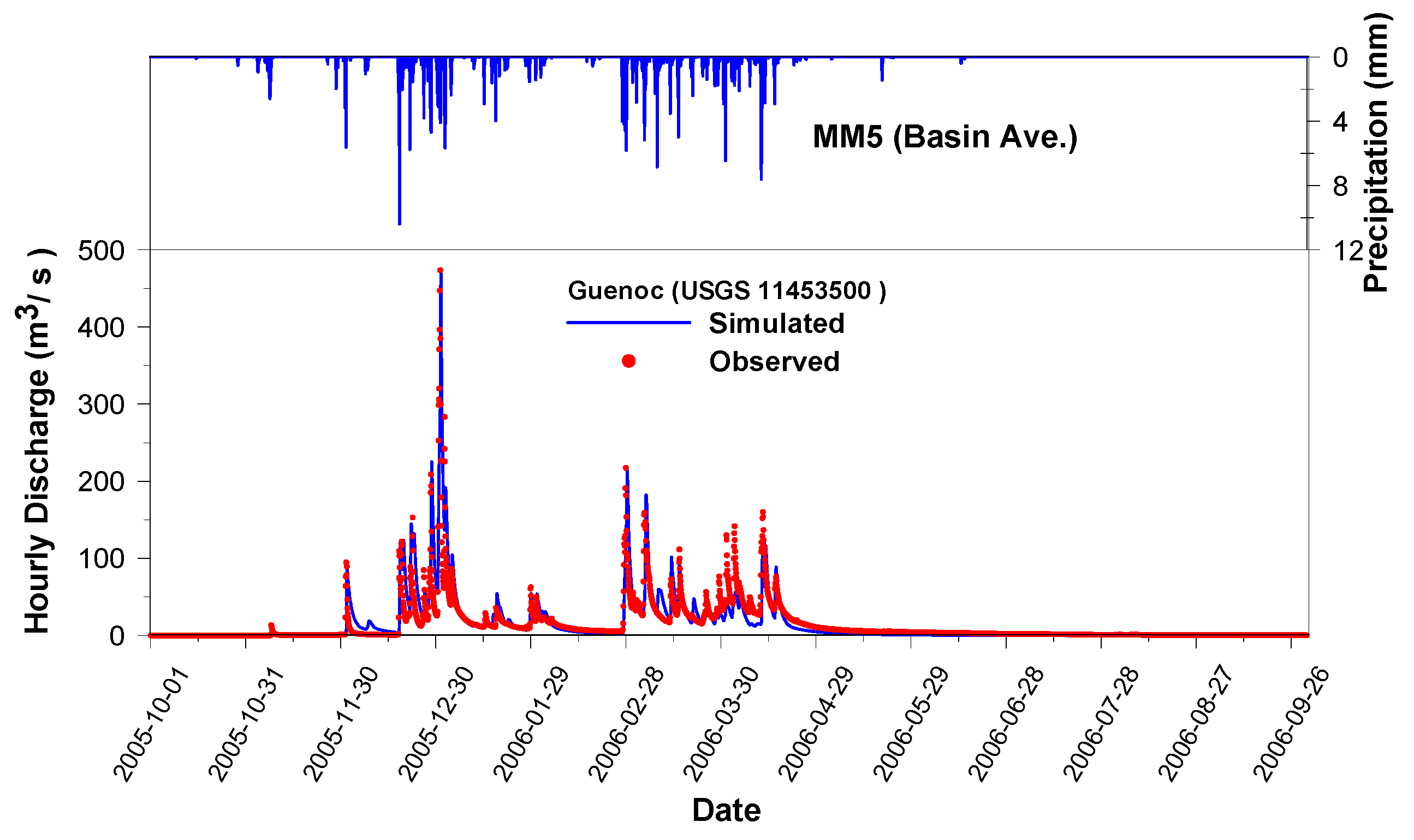
| Statistical Values | Calibration Periods (October 2005–September 2006) | Validation Periods (October 2001–September 2004) |
|---|---|---|
| Mean (observed/simulated) | 14.00/11.67 | 6.63/6.45 |
| STDEV (observed/simulated) | 26.68/27.00 | 18.94/19.26 |
| RMSE | 8.66 | 7.53 |
| Correlation coefficient, R | 0.95 | 0.92 |
| Nash-Sutcliffe efficiency, ENS | 0.89 | 0.84 |
| Volume deviation, Dv (%) | 16.68 | 2.77 |
| Chi-square test, α = 0.05 (critical/calculated) | 18.31/16.08 | 18.31/12.75 |
© 2017 by the authors. Licensee MDPI, Basel, Switzerland. This article is an open access article distributed under the terms and conditions of the Creative Commons Attribution (CC BY) license (http://creativecommons.org/licenses/by/4.0/).
Share and Cite
Jang, S.; Kure, S.; Ohara, N.; Kavvas, M.L.; Chen, Z.Q.; Carr, K.J.; Anderson, M.L. Application of WEHY-HCM for Modeling Interactive Atmospheric-Hydrologic Processes at Watershed Scale to a Sparsely Gauged Watershed. Sustainability 2017, 9, 1554. https://doi.org/10.3390/su9091554
Jang S, Kure S, Ohara N, Kavvas ML, Chen ZQ, Carr KJ, Anderson ML. Application of WEHY-HCM for Modeling Interactive Atmospheric-Hydrologic Processes at Watershed Scale to a Sparsely Gauged Watershed. Sustainability. 2017; 9(9):1554. https://doi.org/10.3390/su9091554
Chicago/Turabian StyleJang, Suhyung, Shuichi Kure, Noriaki Ohara, M. Levent Kavvas, Z. Q. Chen, Kara J. Carr, and Michael L. Anderson. 2017. "Application of WEHY-HCM for Modeling Interactive Atmospheric-Hydrologic Processes at Watershed Scale to a Sparsely Gauged Watershed" Sustainability 9, no. 9: 1554. https://doi.org/10.3390/su9091554