Classification of PolSAR Images Using Multilayer Autoencoders and a Self-Paced Learning Approach

Abstract

In this paper, a novel polarimetric synthetic aperture radar (PolSAR) image classification method based on multilayer autoencoders and self-paced learning (SPL) is proposed. The multilayer autoencoders network is used to learn the features, which convert raw data into more abstract expressions. Then, softmax regression is applied to produce the predicted probability distributions over all the classes of each pixel. When we optimize the multilayer autoencoders network, self-paced learning is used to accelerate the learning convergence and achieve a stronger generalization capability. Under this learning paradigm, the network learns the easier samples first and gradually involves more difficult samples in the training process. The proposed method achieves the overall classification accuracies of 94.73%, 94.82% and 78.12% on the Flevoland dataset from AIRSAR, Flevoland dataset from RADARSAT-2 and Yellow River delta dataset, respectively. Such results are comparable with other state-of-the-art methods.

1. Introduction

Polarimetric synthetic aperture radar (PolSAR) has been one of the most important sensors in remote sensing. In addition to the day–night and all-weather advantages of SAR, PolSAR can transmit and receive electromagnetic energy in more than one polarization. This allows much richer characterization of the observed targets than single-polarization SAR. PolSAR has been proven to be a valuable tool in many areas, such as military, agriculture and environment monitoring [1,2,3,4]. PolSAR image classification is one of the most fundamental issues. With a decade of developments in PolSAR image classification, many effective classification methods have been proposed. Buono et al. [5] used the two most employed unsupervised classification algorithms, namely, the H/a Wishart and the Freeman-Durden Wishart approach, to classify coastal areas, and they evaluated the performance of those classical classifiers over these challenging areas. Xiang et al. [6] presented a new Wishart classification method that used Wishart supervised classification based on the result of H/a-Wishart unsupervised classification. This classification method provides good results in coastal zones. Zhang et al. [7] proposed a supervised PolSAR image classification method that is based on sparse representation. First, the features are extracted. Then, the feature vectors of the training samples construct an over-complete dictionary and obtain the corresponding sparse coefficients; meanwhile, the residual error of the pending pixel with respect to each atom is evaluated and considered as the criteria for classification, and the ultimate class results can be obtained according to the atoms with the least residual error. Du et al. [8] proposed a new method called boosted multiple-kernel extreme learning machines. In this method, Adaptive Boosting was implemented in the training phase, while multiple output fusion strategies, such as Majority Voting, Weighted Majority Voting, MetaBoost, and ErrorPrune were adopted to select the result with the highest overall classification accuracy. Wang et al. [9] proposed a new classification scheme for mud and sand flats on intertidal flats. In this method, Freeman-Durden and Cloude-Pottier polarimetric decomposition components as well as double bounce eigenvalue relative difference were used as features, and random forest theory was used as classification algorithm. Although the above methods have achieved good performance, they still have some limitations. The feature vectors utilized by these methods must be manually constructed, and it is time-consuming to select proper features from various polarization features. In addition, it is challenging to design an appropriate classifier when different types of land cover have similar scattering properties.

In recent years, the booming development of deep learning has motivated many scholars to settle the task by deep learning. Deep learning is fulfilled by a deep neural network (DNN) that has multiple hidden layers and nonlinear activation functions to learn and represent highly nonlinear data. There are many deep learning models, such as autoencoder (AE), deep belief network (DBN) and convolutional neural network (CNN). Xie et al. [10] use the sparse autoencoder (SAE) to extract features from the coherency matrix for terrain classification. Lv et al. [11] proposed a novel classification approach based on DBN. By applying the DBN model, effective spatio-temporal mapping features can be automatically extracted to improve the classification performance. Zhou et al. [12] verify the suitability and effectiveness of CNN in supervised classification of PolSAR images. However, the optimization of DNN is time-consuming, and the quality of the network depends largely on the values in the network initialization. Kumar and Packer et al. [13] have proposed self-paced learning (SPL), which is inspired by the learning process of humans who learn the easier aspects of the task first and then gradually involve more difficult aspects in the training process. This learning paradigm has been empirically demonstrated to be instrumental in accelerating the learning convergence of the network and in weakening the influence of initialization to achieve a stronger generalization capability [14].

In this paper, the classification of PolSAR images based on multilayer autoencoders and self-paced learning (SPLMAE) is proposed. Multilayer autoencoders are a type of unsupervised learning network that converts raw data into more abstract expressions through non-linear models [15]. Several studies have shown the advantages in feature extraction and processing time when using multilayer autoencoders [10,16,17]. The essential idea of multilayer autoencoders is to perform a two-step optimization: pre-training a network layer by layer and fine tuning the network as a classifier. With this two-step optimization, multilayer autoencoders can not only prevent the network from overfitting when the number of labeled samples is relatively small but also extract effective features with its nonlinear mapping ability. Inspired by [18], we use a two-layer autoencoder to learn the features, and a softmax regression is applied to produce the predicted probability distributions over all the classes of each pixel. When optimizing the network, SPL is used to accelerate its learning convergence and achieve a stronger generalization capability.

The remainder of this paper is organized as follows. Section 2 introduces the theory of SPL. Section 3 describes the proposed method. Experiment results on three real PolSAR images are shown in Section 4. Lastly, a brief conclusion is discussed.

2. Related Work

In this section, the key idea of SPL is explained. The goal of SPL is to improve the generalization capability and accelerate the learning convergence through sample selection. Compared with the traditional machine learning methods that consider all samples simultaneously, SPL presents the training data in a meaningful order that facilitates learning, and the order of the samples is determined by the learning difficulty. SPL can trace back to curriculum learning (CL) [19] proposed by Bengio et al. In CL, the order of the training data is unchanged during the iterations. However, SPL dynamically generates the order of the training data according to what the learner has already learned. In [20], Meng et al. ran experiments on various binary classification problems in three University of California Irvine (UCI) datasets (Monk’s problem, Mammographic Mass and SPECT Heart). The experimental results show that the SPL regime can more or less ameliorate the performance (1.63–26.74%) of the traditional classification methods, including logistic regression and support vector classification.

Specifically, in SPL, a weight variable between 0 and 1 is used to denote the learning difficulty of the samples, and a gradually increasing pace parameter is introduced to control the pace at which the model learns new samples. The value of the weight variable is determined by a regularization term called the self-pace regularization term. The model of SPL is formally elaborated below. Given a training dataset $\mathit{D}={\{({\mathit{x}}_i,y_i)\}}_{i=1}^n$, supposed n is the total number of training samples, in which ${\mathit{x}}_i$ denotes the $i^{th}$ observed sample, and $y_i$ represents its label, let $L_i=(y_i,g({\mathit{x}}_i,\mathit{w}))$ denote the loss function, which calculates the training loss (the cost between the ground truth label $y_i$ and the estimated label $g({\mathit{x}}_i,\mathit{w})$). Here, $\mathit{w}$ represents the model parameter inside the decision function $g({\mathit{x}}_i,\mathit{w})$, where $p(\mathit{w})$ is the regularization term imposed on the classifier parameters $\mathit{w}$. Then, a general machine learning framework can be expressed as

$$\mathit{w}=\arg \underset{w}{\min }{\displaystyle \sum _{i=1}^{n}L(y_i,g({\mathit{x}}_i,\mathit{w}))+p(\mathit{w})}$$

(1)

In contrast to Equation (1), the SPL model includes a weighted loss term $v_{i}L(y_i,g({\mathit{x}}_i,\mathit{w}))$ on all samples and a general self-paced regularization term $f(v_i,\lambda )$ imposed on the sample weights $v_i\in [0,1]$, which is expressed as

$$\mathit{w}=\arg \underset{w,v}{\min }{\displaystyle \sum _{i=1}^n{v}_{i}L(y_i,g({\mathit{x}}_i,\mathit{w}))+p(\mathit{w})+f(v_i,\lambda )}$$

(2)

where $\lambda$ is the pace parameter to control the learning process, which will be initialized before training. Here, $f(v_i,\lambda )$ is a regularization term called the self-paced regularization term, which determines the value of the weight $v_i$. The weight $v_i$ is in conformity with the following two rules:

• $v_i$ is monotonically decreasing with respect to the training loss $l_i=L(y_i,g({\mathit{x}}_i,\mathit{w}))$, and it holds that $\underset{l_i->0}{\lim }{v}_i=1$, $\underset{l_i->\infty }{\lim }{v}_i=0$.
• $v_i$ is monotonically increasing with respect to the pace parameter $\lambda$, and it holds that $\underset{\lambda ->0}{\lim }{v}_i=0$, $\underset{\lambda ->\infty }{\lim }{v}_i=1$.

These two rules provide the axiomatic understanding for SPL. Rule (1) indicates that the model is inclined to select easy samples (with smaller training losses). Rule (2) indicates that when the pace parameter $\lambda$ becomes larger, the model tends to incorporate more complex samples to train. Under this axiomatic understanding, Meng, Zhao et al. [20] proposed some typical self-paced regularization terms, and the linear regularization term will be introduced below.

The linear regularization term constrains the relationship between $v_i$ and $l_i=L(y_i,g({\mathit{x}}_i,\mathit{w}))$ into a linear relationship. When the training loss $l_i$ of the $i^{th}$ sample is less than the pace parameter $\lambda$, the weight of this sample is a continuous value between 0 and 1. At each iteration, the weighted samples are used to learn a new parameter vector $\mathit{w}$. The linear regularization term is expressed as follows:

$$f(v_i,\lambda )=\lambda (\frac{1}{2}{v}_i{}^2-v_i)$$

(3)

If we substitute Equation (3) into Equation (2) and simplify, $v_i$ can be obtained by

$$\begin{array}{ll}{v}_i& =\arg \underset{v}{\min }{\displaystyle \sum _{i=1}^n{v}_{i}L(y_i,g({\mathit{x}}_i,\mathit{w}))+p(\mathit{w})-\lambda (\frac{1}{2}{v}_i{}^2-v_i)}\\ & =\arg \underset{v}{\min }{\displaystyle \sum _{i=1}^n{v}_i\left(\frac{1}{2}\lambda v_i+L_i-\lambda \right)+p(\mathit{w})}\\ & \Rightarrow \{\begin{array}{ll}{v}_i=1-\frac{L_i}{\lambda }& if{L}_i<\lambda \\ v_i=0& if{L}_i\ge \lambda \end{array}\end{array}$$

(4)

In SPL, the parameter vector $\mathit{w}$ and $\mathit{v}=[v_1\dots v_i\dots v_n]$ will be calculated iteratively, and the procedure of SPL is as follows:

• Step 1: Initialize the weights of all samples $\mathit{v}$ and parameter $\lambda$.
• Step 2: Fix $\mathit{v}$, and update $\mathit{w}$ by Equation (2).
• Step 3: Fix $\mathit{w}$, calculate the training loss $L(y_i,g({\mathit{x}}_i,\mathit{w}))$, and update $\mathit{v}$ by Equation (4).
• Step 4: If $\mathit{v}$ and $\mathit{w}$ have converged, then go to step 5; otherwise, repeat step 2 and step 3.
• Step 5: Update $\lambda$, $\lambda =\kappa \lambda ,\kappa >1$.
• Step 6: Repeat step 2 to step 5 until the mean of $\mathit{v}$ is equal to or approximately 1. Finally, obtain the solution of $\mathit{w}$.

3. Proposed Method

A new method for PolSAR image classification is proposed in this paper. We use multilayer autoencoders to learn the features for each pixel, and a softmax regression is applied to produce the predicted probability distributions over all the classes of each pixel. To accelerate the learning convergence of the network and achieve a better generalization result, the SPL is introduced when we optimize the multilayer autoencoders network, which learns the easier samples first and then gradually involves more difficult samples in the training process.

3.1. Multilayer Autoencoders Network

In our method, each pixel is represented by a row vector that is extracted from the multi-look coherency matrix T of the PolSAR data, and the row vector is used as the input vector of the network. In the PolSAR data, each pixel is represented as a $2\times 2$ scattering matrix S:

$$\mathbf{S}=\left[\begin{array}{l}{s}_{hh}{s}_{hv}\\ s_{vh}{s}_{vv}\end{array}\right]$$

(5)

where h is the horizontal polarization, and v is the vertical polarization. Therefore, $s_{hv}$ represents the scattering coefficient of the horizontally polarized emission and vertically polarized reception. For the reciprocal backscattering and monostatic radar case, where $s_{hv}=s_{vh}$, the coherency matrix T is obtained by S, which is defined in Equation (6), as follows:

$$\mathbf{T}=\left[\begin{array}{l}{t}_{11},t_{12},t_{13}\\ t_{21},t_{22},t_{23}\\ t_{31},t_{32},t_{33}\end{array}\right]=\frac{1}{2}\left[\begin{array}{ccc}\langle {\left|a\right|}^2\rangle & \langle a{b}^{\prime }\rangle & \langle a{c}^{\prime }\rangle \\ \langle a^{\prime }b\rangle & \langle {\left|b\right|}^2\rangle & \langle b{c}^{\prime }\rangle \\ \langle a^{\prime }c\rangle & \langle b^{\prime }c\rangle & \langle {\left|c\right|}^2\rangle \end{array}\right]$$

(6)

where ′ is the complex conjugate, $a=s_{hv}+s_{vv}$, $b=s_{hh}-s_{vv}$, and $c=2s_{hv}$. The input vector ${\mathit{x}}_i$ is extracted from the coherency matrix T:

$${\mathit{x}}_i=[t_{11},t_{22},t_{33},real(t_{12}),imag(t_{12}),real(t_{13}),imag(t_{13}),real(t_{23}),imag(t_{23})]$$

(7)

Here, real() and imag() represent the real and imaginary parts of the complex number.

$\mathbf{D}={\{({\mathit{x}}_i,y_i)\}}_{i=1}^n$ is the selected training sample set, with n is the total number of training samples, in which ${\mathit{x}}_i$ denotes the $i^{th}$ observed sample’s input vector, and $y_i$ represents its label. Here, we construct a two-layer autoencoders neural network to learn the feature vector of each input vector. Then, a softmax regression is applied to produce the predicted probability distributions over all the classes of each pixel. The two-layer autoencoders with the softmax regression neural network is shown in Figure 1a. In this network, the number of input layer neurons is equal to the dimension of the input vector ${\mathit{x}}_i$, and the number of autoencoder layers and neurons will be determined in our experiment. The number of neurons in the output layer is the number of classes. Here, ${\mathsf{\theta }}^{(k)}$ and ${\mathit{b}}^{(k)}$ ($k\in \{1,2,3\}$) are the parameters of the network. ${\mathsf{\theta }}^{(k)}$ represents the weight matrix of the $k^{th}$ layer, and ${\mathit{b}}^{(k)}$ is the bias vector of the $k^{th}$ layer. The output vector $\mathit{p}$ is the predicted probability distribution over all the classes of input vectors.

3.2. Optimization of Multilayer Autoencoders Network Based on SPL

A two-layer autoencoder with the softmax regression neural network is trained by the following two steps: pre-training the weights and the biases of the network layer by layer and fine tuning those parameters with softmax regression [21]. ${\mathsf{\theta }}^{(k)}$ and ${\mathit{b}}^{(k)}$ ($k\in \{1,2\}$) are optimized by unsupervised pre-training, and then, ${\mathsf{\theta }}^{(k)}$ and ${\mathit{b}}^{(k)}$ ($k\in \{1,2,3\}$) are supervised fine-tuned. The details of the two steps are described as follows.

3.2.1. Unsupervised Pre-Training the Parameters of Each Autoencoder Layer

When pre-training the weights and the biases of the network layer by layer, each autoencoder layer could be considered as an autoencoder. The autoencoder contains an input layer, an encode layer and a decode layer (see Figure 1b), and Figure 1b shows the 1st autoencoder layer of Figure 1a.

The encoding step is

$${\mathit{h}}_i^k=\sigma ({\mathbf{W}}^{(k,1)}{\mathit{x}}_i+{\mathit{b}}^{(k,1)})$$

(8)

where ${\mathbf{W}}^{(k,1)}$ and ${\mathit{b}}^{(k,1)}$ denote the weight matrix and bias vector respectively, $k$ represents the $k^{th}$ autoencoder layer and 1 represents the encode layer, $k\in \{1,2\}$. Here, ${\mathit{x}}^i$ denotes the $i^{th}$ feature vector, and $\sigma$ is an activation function defined by $\sigma (z)=1/(1+e^{-z})$ [22]. ${\mathit{h}}_i^k$ is the $i^{th}$ output vector of the encode layer.

The decoding step is

$${\widehat{\mathit{x}}}_i={\mathbf{W}}^{(k,2)}{\mathit{h}}_i^k+{\mathit{b}}^{(k,2)}$$

(9)

where ${\mathbf{W}}^{(k,2)}$ and ${\mathit{b}}^{(k,2)}$ are the trainable parameters, $k$ represents the $k^{th}$ autoencoder layer and 2 represents the decode layer, $k\in \{1,2\}$. Here, ${\widehat{\mathit{x}}}_i$ is the $i^{th}$ output vector of the decode layer.

Therefore, the cost function of the autoencoder network can be defined as follows:

$$L(\mathbf{W},\mathit{b})=\frac{1}{2}{\Vert {\mathit{x}}_i-{\widehat{\mathit{x}}}_i\Vert }^2$$

(10)

The optimization objective of the autoencoder is to minimize the expectation risk Equation (11) and solve for the parameters W and b.

$$(\mathbf{W},\mathit{b})=\arg \underset{\mathbf{W},\mathit{b}}{\min }\frac{1}{2n}{\displaystyle \sum _{i=1}^n{\Vert {\mathit{x}}_i-{\widehat{\mathit{x}}}_i\Vert }^2}$$

(11)

Stochastic gradient descent and its variants are probably the most used optimization algorithms for deep learning, and mini-batch gradient descent enjoys better convergence rates than stochastic gradient descent in theory. Back propagation algorithm can be used to efficiently compute these gradients [23]. Therefore, back propagation and mini-batch gradient descent are used to train our model. In addition, inspired by the SPL, weighted samples are used to learn the parameter vector in each iteration. Therefore, each sample’s loss $L(\mathbf{W},\mathit{b})$ is multiplied by a weight $v_i$. Then, the cost function $L_{SPL}(\mathbf{W},\mathit{b})$ and optimization objective of SPLMAE of the pre-training can be formulated as in Equations (12) and (13), respectively:

$$L_{SPL}(\mathbf{W},\mathit{b})=v_{i}L(\mathbf{W},\mathit{b})=\frac{1}{2}{v}_i{\Vert {\mathit{x}}_i-{\widehat{\mathit{x}}}_i\Vert }^2$$

(12)

$$(\mathbf{W},\mathit{b})=\arg \underset{\mathbf{W},\mathit{b}}{\min }\frac{1}{2n}{\displaystyle \sum _{i=1}^n{v}_i{\Vert {\mathit{x}}_i-{\widehat{\mathit{x}}}_i\Vert }^2}+f(v_i,\lambda )$$

(13)

The weight $v_i$ represents the $i^{th}$ sample’s learning difficulty in the current iteration, and the easy samples have relatively large weights. Here, $f(v_i,\lambda )$ is the linear SPL regularization term presented in Section 2. When $v_i=0$, the loss incurred by the $i^{th}$ sample is always zero, and when the weight $v_i$ of all samples is equal to 1, Equation (13) can be seen as degenerating to Equation (11). The pace parameter $\lambda$ controls the learning process, and it is initialized before training.

There are three variables (W, b and $v_i$) in the objective function in Equation (13), and it is difficult to optimize these variables at the same time. We can obtain the solution according to the following steps:

• Step 1: initialize the parameters: ${\mathbf{W}}^{(k,1)}$, ${\mathit{b}}^{(k,1)}$, ${\mathbf{W}}^{(k,2)}$, ${\mathit{b}}^{(k,2)}$ and $\lambda$.
• Step 2: apply the mini-batch gradient descent algorithm based on SPL to optimize the parameters.
• Step 2.1: select a mini-batch sample to optimize the parameters.
• Step 2.2: calculate the output vector and loss function for each input vector through forward propagation, and then, calculate the weight parameter $v_i$ by Equation (4).
• Step 2.3: fix the weight parameter $v_i$, and use back propagation to train the parameters ${\mathbf{W}}^{(k,1)}$, ${\mathit{b}}^{(k,1)}$, ${\mathbf{W}}^{(k,2)}$, ${\mathit{b}}^{(k,2)}$.
• Step 2.4: Update $\lambda$, $\lambda =\kappa \lambda ,\kappa >1$. In general, we need the range of training loss values in advance to determine the initial value of $\lambda$ and the step size $\kappa$. In our experiment, the initial value of $\lambda$ is set to the first quartile of the sample training losses, and $\kappa =1.1$.
• Step 2.5: repeat step 2.2 to step 2.4 until the value of $\mathit{v}$ is approximately 1 (all the samples of the current iteration have been completely learned). Here, $\mathit{v}$ is defined as $\mathit{v}=\frac{1}{n}{\displaystyle \sum _{i=1}^n{v}_i}$.
• Step 2.6: a new mini-batch sample is selected to optimize the parameter until all the samples are learned.
• Step 3: repeat step 2 until the number of epochs achieve a predefined threshold, and then, obtain the parameters ${\mathbf{W}}^{(k,1)}$ and ${\mathit{b}}^{(k,1)}$.

3.2.2. Supervised Fine-Tuning Those Parameters with Softmax Regression

The ${\mathbf{W}}^{(k,1)}$ and ${\mathit{b}}^{(k,1)}$ obtained by pre-training are used as the initial parameters of the two-layer autoencoders network shown in Figure 1a. ${\mathsf{\theta }}^{(1)}$ and ${\mathsf{\theta }}^{(2)}$ are initialized by the values of ${\mathbf{W}}^{(1,1)}$ and ${\mathbf{W}}^{(2,1)}$, respectively. Here, ${\mathit{b}}^{(1,1)}$ and ${\mathit{b}}^{(2,1)}$ are used to initialize ${\mathit{b}}^{(1)}$ and ${\mathit{b}}^{(2)}$, respectively. Then, apply supervised fine tuning of the multilayer autoencoders network to update the parameters ${\mathsf{\theta }}^{(k)}$ and ${\mathit{b}}^{(k)}$ ($k\in \{1,2,3\}$). The output layer is a softmax regression classifier, and the number of its neurons is equal to the number of classes. The value of the output vector can be obtained as follows:

$$P({\mathit{h}}_2^{(i)})=\frac{1}{{\displaystyle \sum _{j=1}^c{e}^{{\mathbf{\theta }}_j^{\mathrm{T}}{\mathit{h}}_2^{(i)}}}}{\left[e^{{\mathbf{\theta }}_1^{\mathrm{T}}{\mathit{h}}_2^{(i)}},e^{{\mathbf{\theta }}_2^{\mathrm{T}}{\mathit{h}}_2^{(i)}},\dots ,e^{{\mathbf{\theta }}_c^{\mathrm{T}}{\mathit{h}}_2^{(i)}}\right]}^{\mathrm{T}}$$

(14)

where $P({\mathit{h}}_2^{(i)})$ denotes the predicted probability distributions over all of the classes of the $i^{th}$ sample, and ${\mathit{h}}_2^{(i)}$ is the 2nd layer autoencoder’s output vector of the $i^{th}$ sample. Here, c represents the number of classes, and ${\mathbf{\theta }}_j^{\mathrm{T}}$ (T is the transpose operator) denotes the weight vector of the $j^{th}$ neuron of the output layer. To accelerate the learning convergence and obtain a better locally optimal solution, the optimization objective based on SPL can be formulated as follows:

$$({\mathsf{\theta }}^{(\mathrm{k})},{\mathit{b}}^{(\mathrm{k})})=\arg \underset{{\mathsf{\theta }}^{(\mathrm{k})},{\mathit{b}}^{(\mathrm{k})}}{\min }-\frac{1}{n}\left[{\displaystyle \sum _{i=1}^n{\displaystyle \sum _{j=1}^c{v}_{i}1\{y^{(i)}=j\}\log (\frac{e^{{\mathbf{\theta }}_j^{\mathrm{T}}{\mathit{h}}_2^{(i)}}}{{\displaystyle \sum _{k=1}^c{e}^{{\mathbf{\theta }}_k^{\mathrm{T}}{\mathit{h}}_2^{(i)}}}})+f(v_i,\lambda )}}\right]$$

(15)

where $y^{(i)}$ is the true label of the $i^{th}$ sample, when $y^{(i)}=j$, $1\{y^{(i)}=j\}$ is equal to 1. A two-layer autoencoder with a softmax regression output layer is trained by back propagation and mini-batch gradient descent. The procedure is similar to the pre-training of each autoencoder layer.

4. Experiments

In this section, three real PolSAR data sets are used to validate the performance of the proposed method. In addition, the proposed method is compared with three typical PolSAR classification methods, including SVM [24], Wishart classifier (WC) [25], and Sparse Representation-based classification (SRC) [26]. For the SVM and SRC methods, three polarimetric parameters (entropy, anisotropy and mean scattering angle) extracted by Cloude-Pottier decomposition [27] are used as features. The WC method does not need to extract features, and the coherency matrix is used to classify. For the SVM method, the radial basis function (RBF) kernel is used, the parameter gamma for RBF is 1, and the tolerance of the termination criterion and the cost factor are 0.00001 and 100, respectively. In our experiment, the results of SVM are obtained by the libsvm-3.2 toolbox [28]. For the WC method, the training samples are used to calculate the Wishart centers of each class, and the Wishart distance is used to classify each pixel without iterations. For the SRC method, we use the K-Singular Value Decomposition (K-SVD) [29] algorithm to train an over-complete dictionary. The sparse representation of the test samples is obtained by the orthogonal matching pursuit (OMP) [30] algorithm. In addition, to validate the effectiveness of SPL in neural network optimization, the two-layer autoencoder network without SPL called MAE is used as a comparison algorithm. MAE is also optimized by back propagation and mini-batch gradient descent. All the experiments were performed on an Intel i5-6500 CPU 3.2 GHz, and the code was written with the MATLAB R2015b development environment.

4.1. Network Architecture Analysis

For the multilayer autoencoders network, the numbers of neurons and layers are vital; they affect the quality of the network recovered by the training process and its ability to classify the test dataset [18]. To obtain better classification results, the numbers of neurons and layers are determined by the experiments. This experiment is conducted on the Flevoland dataset from AIRSAR, and this dataset will be described in detail in Section 4.2. In this experiment, we fix the same number of neurons for all layers and train the network by varying the numbers of neurons and layers. The overall accuracy (OA) of the Flevoland dataset obtained by the network with different parameters is shown in Figure 2. In Figure 2, the x-axis and y-axis represent the number of neurons and OA, respectively. The red line represents the single layer autoencoder network; the blue line and black line represent the 2-layer and 3-layer autoencoder network, respectively. The number of neurons ranges from 10 to 130. As shown in the figure, the 2-layer autoencoder network with 90 neurons obtains the highest accuracy (approximately 0.94). The single layer autoencoder network with any number of neurons cannot obtain a good accuracy due to its poor fitting capability. With the increase in the autoencoder layer, the network has better fitting capability. However, the larger the number of network layers, the larger the number of labeled samples that are needed. The black line shows that the 3-layer autoencoder network is worse than the 2-layer autoencoder network. This finding could be due to the overfitting problem because the number of training samples with labels is relatively small. In the synthesis of the factor, the numbers of layers and neurons are set to 2 and 90, respectively.

4.2. Flevoland Dataset from AIRSAR

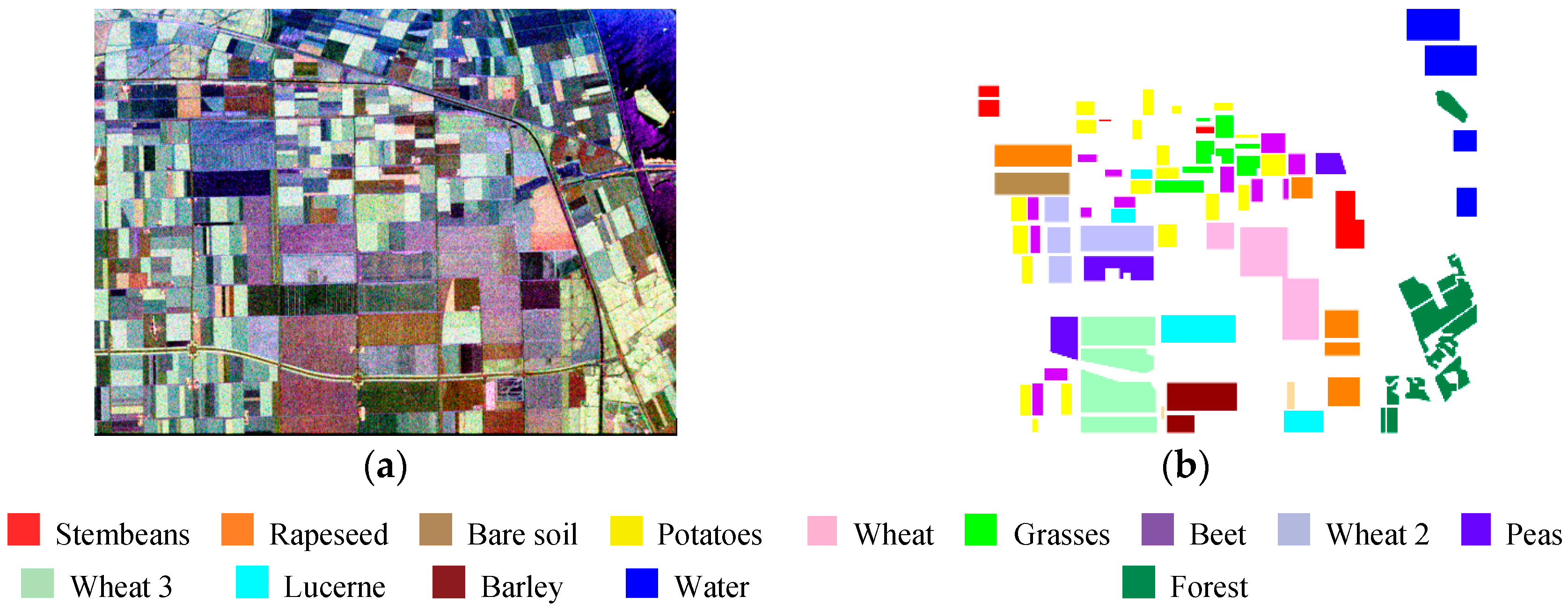
Here, we used the NASA/JPL AIRSAR L-Band four-look PolSAR dataset of Flevoland, the Netherlands, which has the size of 1024 × 750 pixels. The pixel size is 6.6 m in the slant range direction and 12.10 m in the azimuth direction. Figure 3 illustrates the corresponding Pauli RGB image and ground truth (the ground truth is obtained from reference [31]). There are 14 classes in this ground truth, where each class indicates a type of land covering and is identified by one color. A total of 167,712 pixels are labeled in the ground truth, and 15% of them are used to train the network (the training samples are randomly selected). The reported testing accuracies are obtained by testing on the 85% residual pixels. The SPLMAE and MAE is trained by mini-batch gradient descent with an adaptive learning rate, the batch size is 256, and the number of epochs is 3000. The initial learning rate is 1, and after each iteration, the new learning is equal to the learning rate multiplied by 0.999.

4.2.1. Convergence Analysis of Our Algorithm

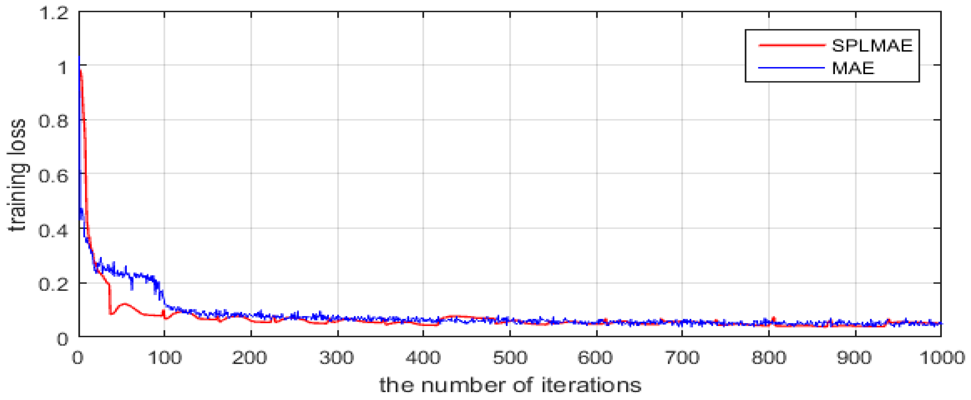
Figure 4 shows that the average training loss of all the training samples (y-axis) varies with the number of epochs (x-axis) in the fine tuning process. The red line represents the optimization process of SPLMAE, and the blue line is the optimization process of MAE. As shown in the two curves, SPLMAE converges faster than MAE. The average training loss is below 0.5 at approximately the 1200th epoch in the red line, but the MAE requires 1500 epochs. In addition, the training loss of the proposed method eventually converges to a lower value than the MAE. In time, as shown in

Table 1. The accuracies of the Flevoland dataset from AIRSAR. AA: average accuracy; OA: overall accuracy.

Class	SVM	SRC	WC	MAE	SPLMAE
Stembeans	0.9719	0.9642	0.9508	0.9842	0.9801
Rapeseed	0.7351	0.6049	0.7484	0.8487	0.9003
Bare soil	0.9802	0.9211	0.9920	0.9039	0.8649
Potatoes	0.9811	0.6631	0.8775	0.9858	0.9815
Beet	0.9541	0.9561	0.9513	0.9679	0.9713
Wheat 2	0.7875	0.7797	0.8272	0.8582	0.8559
Peas	0.9258	0.9396	0.9628	0.9664	0.9676
Wheat 3	0.9288	0.8226	0.8864	0.9732	0.9749
Lucerne	0.9292	0.9513	0.9293	0.9553	0.9608
Barley	0.9365	0.9322	0.9526	0.9738	0.9795
Wheat	0.8128	0.7610	0.8622	0.9656	0.9592
Grasses	0.8373	0.6284	0.7246	0.8203	0.8555
Forest	0.7562	0.9797	0.8791	0.9601	0.9707
Water	0.8213	0.8002	0.5175	0.7981	0.9434
AA	0.8827	0.8360	0.8616	0.9258	0.9404
OA	0.8708	0.8231	0.8504	0.9304	0.9473
Train + Test time (s)	1.3 + 17	84 + 155	130	1539 + 3.4	1495 + 3.5

, SPLMAE reduces the time-consumption slightly compared with MAE. However, both SPLMAE and MAE spend more time in training than SVM and SRC.

4.2.2. Classification Results

Figure 5 shows the visual classification results of the Flevoland dataset, and the accuracies for each class are listed in Table 1. The SVM method is an effective algorithm in the field of classification. It obtains a notably good result with an overall accuracy of 0.8708. As shown in Figure 5a–c, there is less misclassification in the Potatoes, Wheat 3 and Grasses categories in the result obtained from SVM than from SRC and WC. The results of SRC show that most of the Rapeseed, Potatoes and Grasses are misclassified to other categories. The result of the MAE method, shown in Figure 5d, is better than those of SVM, SRC and WC, because the features learned by the multilayer autoencoder network from raw data are better than the shallow features extracted by polarization decomposition. The proposed method SPLMAE has the highest overall accuracy, 0.9473, among all the algorithms, and this result has better performances on most classes, including Rapeseed, Grasses, and Water. In the Water category (see red circles in Figure 5), the compared methods misclassify some Water pixels to Bare soil. Our proposed approach outperforms MAE, which validates the effectiveness of SPL in helping the network to achieve a stronger generalization capacity. The running times for each method are listed in Table 1. MAE and SPLMAE spend more time on training than SVM and SRC. However, SVM and SRC need more time on testing and the extra time of SVM and SRC on feature extraction is not included in Table 1.

4.3. Flevoland Dataset from RADARSAT-2

The Flevoland Dataset from RADARSAT-2 is C-band single-look fully PolSAR data with a resolution of 10 × 5 m and was obtained at fine quad-mode in 2008. A sub-region with 1200 × 1400 pixels was selected, as shown in Figure 6a, and the ground-truth datum is shown in Figure 6b, with the ground truth obtained from [32]. There are four main types of terrain as follows: (1) forest; (2) cropland; (3) water; and (4) urban area. Approximately 5% of the labeled samples are randomly selected to train the network. The SPLMAE and MAE are trained by mini-batch gradient descent with an adaptive learning rate, and the batch size is 256. The algorithm converges more readily in the second experiment than in the first, and therefore, the number of epochs was set to 50. The initial learning rate is 1, and after each iteration, the new learning was equal to the learning rate multiplied by 0.999.

Figure 7 shows the descent curve of the average training loss of Flevoland dataset from RADARSAT-2. This dataset is not especially challenging, and most areas such as forest, water and cropland are homogeneous regions, and their scattering characteristics have obvious differences. When optimizing this dataset, our model converges at the 30th epoch. Therefore, to clearly show the descent curve of the training loss, the x-axis represents the number of iterations (the number of parameter updates) and not epochs. As shown in this figure, the SPLMAE converges faster than MAE. Both SPLMAE and MAE could eventually converge to a low training loss. Figure 6c–g shows the visual classification results, and

Table 2. The accuracies of Flevoland dataset from RADARSAT-2. AA: average accuracy; OA: overall accuracy.

Class	SVM	SRC	WC	MAE	SPLMAE
Urban	0.8051	0.7579	0.6022	0.8712	0.8921
Water	0.9693	0.9779	0.9854	0.9878	0.9870
Forest	0.9207	0.9195	0.8479	0.9537	0.9468
Cropland	0.9372	0.8759	0.8071	0.9327	0.9408
AA	0.9080	0.8828	0.8107	0.9363	0.9417
OA	0.9229	0.8978	0.8382	0.9449	0.9482
Train + Test time (s)	1+ 11.7	26 + 436	87.5	51 + 5	42 + 4.7

shows the accuracies for each class. The proposed method SPLMAE has the best visual effect and the highest overall accuracy, 0.9482, compared with other algorithms. The accuracy benefits from the better performances on the urban areas (see white circles in Figure 6c–g). The urban areas have a mixed scattering mechanism that is more difficult to classify than the other categories. The results of SVM, SRC and WC show that most of the Urban areas are misclassified to Forest. However, when employing the features that are learned by our network, it can effectively classify this area, as in Figure 6f,g. This dataset is not especially challenging, and the scattering characteristics of different categories have obvious differences. Therefore, the result of SPLMAE is a slight improvement against the result of MAE.

4.4. Yellow River Delta Dataset from ALOS-2

To validate the performance of the SPLMAE on scenes that are characterized by several types of land cover with similar scattering properties, an ALOS-2 fully PolSAR image acquired on 9 May 2015 over the Yellow River Delta, China (see Figure 8a) is also considered. The size of the image is 23,210 × 7496 pixels. The pixel spacing is 3.125 m. The study area is a coastal region that is covered with different land-use types. The regions of interest include coastal shoal, alkali soil, wetland, plantation, pond, and river (see Figure 8b). Classifying different types of land cover in coastal zones using SAR imagery is a challenge because many types of coastal zone have similar backscattering characteristics. Most of the classification algorithms are based on the intensity of the image, and they do not perform well in different coastal zone types [33,34]. Considering the limited memory, we intercept the sub-areas that have different land-use types in the image, as is shown in the red rectangle of Figure 8a,b, where the size of the sub-image is 2000 × 5000.

The classification results of this sub-image are shown in Figure 9. Table 2 shows the accuracies and running time for each method. SVM can classify the pond, alkali soil and coastal shoal well but not the plantation and river (see the red circles in Figure 9b). However, SRC cannot classify most of the categories and the result contains a lot of noise. The result of WC (see Figure 9d) is quoted from referenced [5]. WC has the ability to recognize wetland and plantation but pond, alkali soil, coastal shoal and river are classified into the same class. Different land cover in this dataset have similar scattering characteristics, and it is more difficult to distinguish them. SPLMAE and MAE achieve better results in each class than the other methods, which shows that the features extracted by multilayer autoencoders are effective over these challenging areas. In addition, according to Figure 9e,f and the accuracies of SPLMAE and MAE (

Table 3. The accuracies of the Yellow River Delta. AA: average accuracy; OA: overall accuracy.

Class	SVM	SRC	WC	MAE	SPLMAE
Pond	0.8540	0.3680	--	0.9230	0.9132
Alkali Soil	0.8498	0.4681	--	0.8350	0.8523
Coastal Shoal	0.7192	0.4912	--	0.7798	0.7758
Wetland	0.5544	0.2311	--	0.5908	0.6678
Plantation	0.5280	0.4377	--	0.7175	0.7124
River	0.1444	0.3144	--	0.3215	0.4489
AA	0.6083	0.3851	0.6	0.6946	0.7284
OA	0.7113	0.3963	--	0.7627	0.7812
Train + Test time (s)	5 + 305	39 + 2871	--	5840 + 52	5643 + 53

), we can conclude that the network optimized under SPL regime can obtain a better solution. The running times of each method are listed in Table 3. MAE and SPLMAE spend more time on training than SVM and SRC. However, SVM and SRC need more time on testing and the extra time of SVM and SRC on feature extraction is not included in Table 3.

5. Conclusions

In this paper, a classification method based on the SPL algorithm and multilayer autoencoders network is proposed for PolSAR image classification. In the proposed model, a two-layer autoencoder is used to learn the features, and a softmax regression is applied to produce the predicted probability distributions over all the classes of each pixel. When we optimize the network, SPL is used to accelerate the learning convergence of a network and achieve a stronger generalization capacity. According to the experimental results presented above, we can draw the following conclusions.

First, SPLMAE obtained better classification results than conventional algorithms such as SVM, SRC and WC because it can extract more abstract and effective features. The abstract features can better reveal the differences between different classes, which makes terrains easier to classify. The proposed method spends more time on training than SVM and SRC but saves extra time for feature extraction and feature selection. Second, SPLMAE works even better compared to MAE. Although MAE can also extract deep features, the quality of the network depends largely on the value of the network initialization. SPL is instrumental in accelerating the learning convergence of a network and in weakening the influence of initialization to achieve a stronger generalization capacity. Therefore, SPLMAE converges faster than MAE (see Figure 4 and Figure 6) and has better visual classification results, especially in some scenes that are characterized by several types of land cover that have similar scattering properties. In addition, the proposed method performs well on the first two datasets collected over the same area at different frequencies, which proves the robustness of our method with regard to variations in the frequency.

The spatial information in the PolSAR data is useful for classification. However, the input of the multilayer autoencoder must be a one-dimensional vector instead of image patches, which cannot exploit the spatial information very well. Zhou et al. [12] proposed that the CNN can automatically learn hierarchical polarimetric spatial features from the raw data. Therefore, we plan to investigate classification techniques based on the CNN, autoencoder and SPL in terms of future research.

References

- Liu, F.; Jiao, L.; Hou, B.; Yang, S. POL-SAR image classification based on Wishart DBN and local spatial information. IEEE Trans. Geosci. Remote Sens. 2016, 54, 3292–3308. [Google Scholar] [CrossRef]
- Nunziata, F.; Migliaccio, M.; Li, X.; Ding, X. Coastline extraction using dual-polarimetric COSMO-SkyMed PingPong mode SAR data. IEEE Geosci. Remote Sens. Lett. 2014, 11, 104–108. [Google Scholar] [CrossRef]
- Ding, X.; Li, X. Shoreline movement monitoring based on SAR images in Shanghai, China. Int. J. Remote Sens. 2014, 35, 3994–4008. [Google Scholar] [CrossRef]
- Ding, X.; Li, X. Monitoring of the water-area variations of Lake Dongting in China with ENVISAT ASAR images. Int. J. Appl. Earth Obs. Geoinform. 2011, 13, 894–901. [Google Scholar] [CrossRef]
- Buono, A.; Nunziata, F.; Migliaccio, M.; Yang, X.; Li, X. Classification of the Yellow River delta area using fully polarimetric SAR measurements. Int. J. Remote Sens. 2017, 38, 6714–6734. [Google Scholar] [CrossRef]
- Xiang, H.; Liu, S.; Zhuang, Z.; Zhang, N. A classification algorithm based on Cloude decomposition model for fully polarimetric SAR image. IOP Conf. Ser. Earth Environ. Sci. 2016, 46. [Google Scholar] [CrossRef]
- Zhang, L.; Sun, L.; Zou, B. Fully polarimetric SAR image classification via sparse representation and polarimetric features. IEEE J. Sel. Top. Appl. Earth Obs. Remote Sens. 2015, 8, 7978–7990. [Google Scholar] [CrossRef]
- Du, P.; Samat, A.; Gamba, P.; Xie, X. Polarimetric SAR image classification by boosted multiple-kernel extreme learning machines with polarimetric and spatial features. Int. J. Remote Sens. 2014, 35, 7978–7990. [Google Scholar] [CrossRef]
- Wang, W.; Yang, X.; Li, X. A Fully Polarimetric SAR Imagery Classification Scheme for Mud and Sand Flats in Intertidal Zones. IEEE Trans. Geosci. Remote Sens. 2017, 55, 1734–1742. [Google Scholar] [CrossRef]
- Xie, H.; Wang, S.; Liu, K.; Lin, S.; Hou, B. Multilayer feature learning for polarimetric synthetic radar data classification. In Proceedings of the IEEE Conference on International Geoscience and Remote Sensing Symposium (IGARSS), Quebec City, QC, Canada, 13–18 July 2014; pp. 2818–2821. [Google Scholar]
- Lv, Q.; Dou, Y.; Niu, X. Classification of land cover based on deep belief networks using polarimetric RADARSAT-2 data. In Proceedings of the IEEE Conference on International Geoscience and Remote Sensing Symposium (IGARSS), Quebec City, QC, Canada, 13–18 July 2014; pp. 4679–4682. [Google Scholar]
- Zhou, Y.; Wang, H.; Xu, F. Polarimetric SAR image classification using deep convolutional neural networks. IEEE Geosci. Remote Sens. Lett. 2016, 13, 1935–1939. [Google Scholar] [CrossRef]
- Kumar, M.P.; Packer, B.; Koller, D. Self-paced learning for latent variable models. In Proceedings of the Conference on Advances in Neural Information Processing Systems (NIPS), Vancouver, BC, Canada, 6–9 December 2010; pp. 1189–1197. [Google Scholar]
- Tang, Y.; Yang, Y.B.; Gao, Y. Self-paced dictionary learning for image classification. In Proceedings of the ACM International Conference on Multimedia, Nara, Japan, 29 October–2 November 2012; pp. 833–836. [Google Scholar]
- Kang, M.; Ji, K.; Leng, X. Synthetic Aperture Radar Target Recognition with Feature Fusion Based on a Stacked Autoencoder. Sensors 2017, 17, 192. [Google Scholar] [CrossRef] [PubMed]
- Ranzato, M.A.; Szummer, M. Semi-supervised learning of compact document representations with deep networks. In Proceedings of the International Conference on Machine Learning (ICML), Helsinki, Finland, 5–9 July 2008; pp. 792–799. [Google Scholar]
- Huang, F.J.; Boureau, Y.L.; LeCun, Y. Unsupervised learning of invariant feature hierarchies with applications to object recognition. In Proceedings of the IEEE Conference on Computer Vision and Pattern Recognition (CVPR), Minneapolis, MI, USA, 12–22 June 2007; pp. 1–8. [Google Scholar]
- Hou, B.; Kou, H.D. Classification of polarimetric SAR image using multilayer autoencoders and superpixels. IEEE J. Sel. Top. Appl. Earth Obs. Remote Sens. 2016, 9, 3072–3081. [Google Scholar] [CrossRef]
- Bengio, Y.; Louradour, J. Curriculum learning. In Proceedings of the International Conference on Machine Learning (ICML), Montreal, QC, Canada, 14–18 June 2009; pp. 41–48. [Google Scholar]
- Meng, D.Y.; Zhao, Q.; Jiang, L. What objective does self-paced learning indeed optimize? arXiv, 2015; arXiv:1511.06049. [Google Scholar]
- Rifai, S.; Mesnil, G.; Vincent, P.; Muller, X.; Bengio, Y.; Dauphin, Y.; Glorot, X. Higher order contractive auto-encoder. In Proceedings of the European Conference on Machine Learning and Principles and Practice of Knowledge Discovery in Databases (ECML PKDD), Athens, Greece, 5–9 September 2011; pp. 645–660. [Google Scholar]
- LeCun, Y.; Bengio, Y.; Hinton, G. Deep learning. Nature 2015, 521, 436–444. [Google Scholar] [CrossRef] [PubMed]
- Goodfellow, I.; Bengio, Y.; Courville, A. Deep Learning; MIT Press: Cambridge, MA, USA, 2016; pp. 203–218, 277–282. ISBN 9780262337434. [Google Scholar]
- Lardeux, C.; Frison, P.L.; Tison, C. Support vector machine for multifrequency SAR polarimetric data classification. IEEE Trans. Geosci. Remote Sens. 2009, 47, 4143–4152. [Google Scholar] [CrossRef]
- Lee, J.S.; Grunes, M.R.; Ainsworth, T.L. Unsupervised classification using polarimetric decomposition and the complex wishart classifier. IEEE Trans. Geosci. Remote Sens. 1999, 37, 2249–2258. [Google Scholar]
- Feng, J.; Cao, Z.; Pi, Y. Polarimetric contextual classification of PolSAR images using sparse representation and superpixels. Remote Sens. 2014, 6, 7158–7181. [Google Scholar] [CrossRef]
- Cloude, S.R.; Pottier, E. An entropy based classification scheme for land applications of Polarimetric SAR. IEEE Trans. Geosci. Remote Sens. 1997, 35, 68–78. [Google Scholar] [CrossRef]
- Chang, C.C.; Lin, C.J. LIBSVM: A library for support vector machines. ACM Trans. Intell. Syst. Technol. 2011, 2, 1–27. [Google Scholar] [CrossRef]
- Aharon, M.; Elad, M.; Bruckstein, A. K-SVD: An algorithm for designing overcomplete dictionaries for sparse representation. IEEE Trans. Signal Proc. 2006, 54, 4311–4322. [Google Scholar] [CrossRef]
- Pati, Y.C.; Rezaiifar, R.; Krishnaprasad, P.S. Orthogonal matching pursuit: Recursive function approximation with applications to wavelet decomposition. In Proceedings of the IEEE Asilomar Conference on Signals, Systems and Computers, Pacific Grove, CA, USA, 1–3 November 1993; pp. 40–44. [Google Scholar]
- Ainsworth, T.; Kelly, J.; Lee, J.S. Classification comparisons between dual-pol, compact polarimetric and quad-pol SAR imagery. ISPRS J. Photogramm. Remote Sens. 2009, 64, 464–471. [Google Scholar] [CrossRef]
- Uhlmann, S.; Kiranyaz, S. Integrating color features in polarimetric SAR image classification. IEEE Trans. Geosci. Remote Sens. 2014, 52, 2197–2216. [Google Scholar] [CrossRef]
- Buono, A.; Nunziata, F.; Mascoloand, L.; Migliaccio, M. A multi-polarization analysis of coastline extraction using X-band COSMO-SkyMed SAR data. IEEE J. Sel. Top. Appl. Earth Obs. Remote Sens. 2014, 7, 2811–2820. [Google Scholar] [CrossRef]
- Gou, S.P.; Yang, X.F.; Li, X.F. Coastal zone classification with full-polarization SAR imagery. IEEE Geosci. Remote Sens. Lett. 2016, 13, 1616–1620. [Google Scholar] [CrossRef]
Figure 1.
(a) Two-layer autoencoder with softmax regression neural network; (b) 1st autoencoder network.
Figure 2.
The performance analysis of the networks with different architectures.
Figure 3.
(a) Pauli RGB; (b) Ground truth; white area denotes unlabeled pixels.
Figure 4.
The convergence analysis of the Flevoland dataset from AIRSAR.
Figure 5.
The classification results of the Flevoland dataset from AIRSAR. (a) SVM, OA = 0.8708; (b) SRC, OA = 0.8231; (c) WC, OA = 0.8504; (d) MAE, OA = 0.9304; (e) SPLMAE, OA = 0.9473.
Figure 6.
The classification results of the Flevoland dataset from RADARSAT-2. (a) Pauli RGB; (b) Ground truth; black area denotes unlabeled pixels; (c) SVM, OA = 0.9229; (d) SRC, OA = 0.8231; (e) WC, OA = 0.8382; (f) MAE, OA = 0.9449; (g) SPLMAE, OA = 0.9482.
Figure 7.
The convergence analysis of the Flevoland dataset from RADARSAT-2.
Figure 8.
(a) Yellow River Delta dataset; (b) Official land use of study area generated for 2015.
Figure 9.
The classification results of the sub-image. (a) Pauli RGB; (b) SVM; (c) SRC; (d) WC; (e) MAE; (f) SPLMAE.