Band Subset Selection for Hyperspectral Image Classification

Abstract

This paper develops a new approach to band subset selection (BSS) for hyperspectral image classification (HSIC) which selects multiple bands simultaneously as a band subset, referred to as simultaneous multiple band selection (SMMBS), rather than one band at a time sequentially, referred to as sequential multiple band selection (SQMBS), as most traditional band selection methods do. In doing so, a criterion is particularly developed for BSS that can be used for HSIC. It is a linearly constrained minimum variance (LCMV) derived from adaptive beamforming in array signal processing which can be used to model misclassification errors as the minimum variance. To avoid an exhaustive search for all possible band subsets, two numerical algorithms, referred to as sequential (SQ) and successive (SC) algorithms are also developed for LCMV-based SMMBS, called SQ LCMV-BSS and SC LCMV-BSS. Experimental results demonstrate that LCMV-based BSS has advantages over SQMBS.

1. Introduction

Hyperspectral image classification has received considerable interest in recent years [1,2,3,4,5,6,7,8,9,10,11,12,13,14,15,16,17,18,19,20,21,22,23]. Its band selection (BS) issue has been also studied extensively [24,25,26,27,28,29,30,31,32,33,34,35,36,37,38,39,40,41,42,43,44,45,46,47,48,49,50,51,52,53,54,55,56,57]. In general, there are two approaches to BS. One is to select bands one at a time, sequentially; this is referred to as sequential multiple band selection (SQMBS). In this case, a criterion that can be used to select bands, according to priorities ranked by the criterion, is usually required. Such a criterion is referred to as a band prioritization (BP) criterion, and it can be designed according to two perspectives. One type of BP criterion is based on data characteristics or statistics such as variance, signal-to-noise ratio (SNR), entropy, and information divergence (ID) to calculate a priority score for each of the individual bands in order to rank them [25]. As a result, such BP-based SQMBS is generally unsupervised and is not adaptive to any particular application. In other words, the same selected bands are also applied to all different applications. The other type of BP criterion is supervised and is adaptive to a particular application, such as classification [26,27,28,29,30,31,32,33,34,35,36,37,38,39,40,41,42,43,44,45,46,47,48,49,50,51,52,53,54,55,56,57], target detection [49,50], endmember extraction [51], spectral unmixing [52], etc. Unfortunately, one of major problems with BP-derived BS methods is how to deal with band correlation. Since hyperspectral imagery has very high interband correlation, the fact that a band has a high priority to be selected implies that its adjacent bands also have high priorities to be selected. To avoid this dilemma, band decorrelation may be required to remove redundant bands from a group of selected bands. However, this also comes with two issues, i.e., how to select a band correlation criterion to measure the correlation between two bands, and how to determine the threshold for two bands that are sufficiently decorrelated.

As an alternative to BP-based SQMBS methods, another approach, referred to as simultaneous multiple band selection (SMMBS), is to select multiple bands simultaneously as a band subset. This approach does not have issues in prioritizing bands or decorrelating bands that are encountered in SQMBS. However, the price paid for these advantages is how to develop an effective search strategy to find an optimal band subset, since it generally requires an exhaustive search, which is practically infeasible. To address this issue, several works have been recently proposed, such as band clustering [58,59,60], particle swarm optimization (PSO) in [35], firefly algorithm (FA) in [36], multitask sparsity pursuit (MTSP) [38], multigraph determinantal point process (MDPP) [43], dominant set extraction BS (DSEBS) in [40], etc. Of particular interest is a new concept of band subset selection (BSS) to address this issue which is quite different from the aforementioned SMMBS methods in the sense of the search strategy to be used for finding an optimal set of multiple bands. It considers a selected band as a desired endmember. Accordingly, finding an optimal set of endmembers from all data sample vectors can be translated to selecting an optimal band subset simultaneously from all bands. With this interpretation, two sequential algorithms designed to realize an N-finder algorithm (N-FINDR) [61] numerically, called sequential N-FINDR (SQ N-FINDR) and successive N-FINDR (SC N-FINDR) [62,63,64,65] can be redesigned to find desired band subsets, called SQ BSS and SC BSS algorithms. These two SQ BSS and SC BSS algorithms were recently developed for SMMBS in applications of anomaly detection [66] and spectral unmixing and classification [67,68]. This paper further extends BSS to hyperspectral image classification and has several different aspects not found in [66,67,68]. First and foremost is the criterion used for BSS, which is the minimum variance resulting from a linearly constrained finite impulse response filter arising in adaptive beamforming in array signal processing [69,70,71,72]. This linearly constrained minimum variance (LCMV)-based BSS interprets signal sources as class signature vectors and linearly constrains the class signature vectors, finding an optimal band subset for classification. It is very different from constrained energy minimization (CEM)-based BS [26], which constrains a single selected band, and also from constrained multiple band selection (CMBS) [68], which extends CEM-BS by constraining multiple bands as band subsets, not as class signature vectors as LCMV-BSS does. Secondly, two new SQ BSS and SC BSS algorithms are developed for LCMV-BSS, specifically for classification, referred to as SQ LCMV-BSS and SC LCMV-BSS. Thirdly, the classifier used to evaluate BS performance is also an LCMV classifier which is particularly designed to best utilize the bands selected by LCMV-BSS. Fourthly, despite the fact that LCMV-BSS may not exhaust all possible band combinations, to the authors’ best knowledge, LCMV-BSS is probably the only BSS algorithm to search band subsets among all possible band combinations numerically compared to other SMMBS algorithms such as PSO, FA, MTSP, MDPP, DSEBS which are indeed designed to run only a very small selected set of band subsets. Finally, and most importantly, the proposed LVMV-BSS is very easy to implement because there are no parameters that need to be tuned, as many BS methods have. This is a tremendous advantage since such parameters must be adaptive to various applications.

2. LCMV Criterion for BSS

Suppose that there are M classes of interest and each class is specified by a class signature vector, denoted by $d_1,\hspace{0.17em}{d}_2,\hspace{0.17em}\cdots ,\hspace{0.17em}{d}_M$. We can now form a class signature matrix, denoted by $D=\left[d_1{d}_2\cdots d_M\right]$. The goal is to design an FIR linear filter with L filter coefficients $\{w_1,\hspace{0.17em}{w}_2,\hspace{0.17em}\cdots ,\hspace{0.17em}{w}_L\}$, denoted by an L-dimensional vector $w=\left(w_1{w}_2\cdots w_L\right){}^T$ that minimizes the filter output energy subject to the following constraint:

$$D^{T}w=c \mathrm{where} d_j^{T}w={\displaystyle {\sum }_{l=1}^L{w}_l{t}_{jl}} \mathrm{for} 1\le j\le M$$

(1)

where $c=\left(c_1{c}_2\cdots c_k\right){}^T$ is a constraint vector. Using (1), we derive the following linearly constrained optimization problem:

$${\min }_w\left\{w^{T}Rw\right\} \mathrm{subject} \mathrm{to}{D}^{T}w=c$$

(2)

where $R=\left(1/N\right){\displaystyle {\sum }_{i=1}^N{r}_i{r}_i^T}$ is the autocorrelation sample matrix of the image. The solution to (2) is called the LCMV-based classifier and can be obtained in [69,71,72] by

$${\delta }^{\mathrm{LCMV}}(r)={\left(w^{\mathrm{LCMV}}\right)}^{T}r$$

(3)

with

$$w^{\mathrm{LCMV}}=R^{-1}D{\left(D^T{R}^{-1}D\right)}^{-1}c.$$

(4)

Substituting (3) into (4) yields

$$\begin{array}{l}{\left(w^{\mathrm{LCMV}}\right)}^T{R}^{-1}{w}^{\mathrm{LCMV}}\\ ={\left[R^{-1}D{\left(D^T{R}^{-1}D\right)}^{-1}c\right]}^T{R}^{-1}\left[R^{-1}D{\left(D^T{R}^{-1}D\right)}^{-1}c\right]\\ =c^T{\left(D^T{R}^{-1}D\right)}^{-1}{D}^T{R}^{-1}D{\left(D^T{R}^{-1}D\right)}^{-1}c=c^T{\left(D^T{R}^{-1}D\right)}^{-1}c\end{array}.$$

(5)

According to [70], (5) is the minimum variance weighted by $R^{-1}$. As a matter of fact, (5) can be also viewed as the minimal $R^{-1}$-weighted least squares error (LSE) caused by misclassification errors from operating δ^LCMV on the entire image cube. For those who would like to learn more about LCMV, its details can be found in [69,70,71].

3. Band Subset Selection

A BS problem is generally described as follows. Assume that J(.) is a generic objective function of Ω_BS for the BS to be optimized where Ω_BS is a band subset selected from a full band set Ω. For a given number n_BS of selected bands, a BS method is to find an optimal band subset ${\mathbf{\Omega }}_{\mathrm{BS}}^{*}$ with $\left|{\mathbf{\Omega }}_{\mathrm{BS}}\right|=n_{\mathrm{BS}}$ which satisfies the following optimization problem:

$${\mathbf{\Omega }}_{\mathrm{BS}}^{*}=\arg \left\{\max /{\min }_{{\mathbf{\Omega }}_{\mathrm{BS}}\subset \mathbf{\Omega },\left|{\mathbf{\Omega }}_{\mathrm{BS}}\right|=n_{\mathrm{BS}}}J\left({\mathbf{\Omega }}_{\mathrm{BS}}\right)\right\}.$$

(6)

Depending upon how the objective function J(Ω_BS) is designed, the optimization in (6) can be performed by either maximization or minimization over all possible band subsets Ω_BS contained in Ω with $\left|{\mathbf{\Omega }}_{\mathrm{BS}}\right|=n_{\mathrm{BS}}$.

Since solving (6) requires exhausting all possible n_BS-band combinations to find an optimal band subset, ${\mathbf{\Omega }}_{\mathrm{BS}}^{*}$, it is practically impossible to do so. Accordingly, many approaches have been investigated by designing various criteria or features to define J(Ω_BS) and solve (6). One traditional approach is to design a BP criterion to rank all bands from which BS can be carried out by selecting bands according to their calculated priorities by a particular BP criterion. Such an approach generally results in an SQMBS method which selects multiple bands one at a time sequentially. As noted in the introduction, one major issue arising from this approach is how to deal with redundant bands caused by band correlation. As an alternative, another BP-derived SQMBS method is to specify a particular application such as minimum estimated abundance covariance (MEAC) for classification [34], which can generate feature vectors for BP and then takes advantage of the sequential forward floating search (SFFS) and sequential backward floating search (SBFS) developed in [73] to derive forward and backward BS methods. However, the band correlation issue still remains.

In contrast to SQMBS, many recent efforts have been directed to SMMBS, which selects multiple bands simultaneously at the same time. Associated with SMMBS are also two main issues needed to be addressed. One is determining the number n_BS of bands to be selected, which is also an issue in SQMBS. Generally, n_BS can be determined by either trial-and-error or the virtual dimensionality (VD) developed in [69,74]. The other is a more critical issue, which is to how to find appropriate n_BS bands. Suppose that n_BS = p is the number of bands needed to be selected, ${\mathbf{\Omega }}_p=\left\{B_{l_1},B_{l_2},\dots ,B_{l_p}\right\}$ is a p-band band subset selected from a full band set $\mathbf{\Omega }=\left\{B_1,B_2,\cdots ,B_L\right\}$ where L is the total number of bands, and $B_{l_j}$ is the selected jth band. In order to find an optimal band subset ${\mathbf{\Omega }}_p^{*}$, we must run through all possible $\left(\begin{array}{l}L\\ p\end{array}\right)=\frac{L!}{p!(L-p)!}$ p-combinations among L bands. Practically, this is infeasible if L is large such as in hyperspectral imagery. In this case, developing an effective search strategy for finding an optimal set of multiple bands that does not exist in SQMBS is a great challenge to SMMBS.

A simple SMMBS approach is to group or combine bands into clusters, each of which produces a representative band for BS using certain band measure criteria [58,59,60]. In particular, the concept in [58] is similar to Fisher’s ratio, using mutual information as a band prioritization criterion for clustering. Most interestingly, a band group-wise method was developed [38], which used band combinations by compressive sensing and a multitask sparsity pursuit (MTSP)-based criterion to select band combinations based on linear sparse representation via an evolution-based algorithm-derived search strategy. Another SMMBS approach is to narrow the search range by specifying particular parameters to limit a small number of band subsets as candidate optimal sets, then follow an optimization algorithm such as PSO [35] or FA [36] to find an optimal band subset from the selected candidate set of band subsets.

Most recently, two other promising approaches have been reported. One is to use graph-based representations with each path used to specify a particular band subset. For example, Yuan et al. [43] proposed a graph-based SMMBS method, called multigraph determinantal point process (MDPP), which makes use of multiple graphs to discover a structure and diverse band subset from a graph where each node represents a band and the edges are specified by similarity between bands. Accordingly, a path represents a possible band subset. Then, a search algorithm called mixture determinantal point process (Mix-DPP) was further developed to find a diverse subset that can be a potential optimal band combination. The other is DSEBS, which exploits structure information via a set of local spatial–spectral filters and uses a graph-based clustering search strategy derived from dominant set extraction to find a potential optimal band subset [40].

In addition to the above-mentioned approaches there is also a new approach, called BSS, which considers the problem of multiple band selection as an endmember finding problem. If a desired selected band is interpreted as an endmember and the full band set as the entire data set, then a band subset can be interpreted as a set of endmembers. Consequently, finding an optimal set of n_BS bands can be carried out in a similar way to finding an optimal set of n_BS endmembers. This BSS-based approach has recently proved to be very promising and has great potential in various applications such as anomaly detection in [65], spectral unmixing in [66], and target detection in [67]. This paper presents another new application of BSS to hyperspectral image classification with LCMV used as a criterion particularly designed for classification.

4. LCMV-BSS Algorithms

Now, if we replace the full band set Ω in $R^{-1}$ of (5) with a selected band subset Ω_BS, then (5)

$$\mathrm{MV}({\mathbf{\Omega }}_{\mathrm{BS}})={\mathbf{c}}^T{\left({\mathbf{D}}_{{\mathbf{\Omega }}_{\mathrm{BS}}}^T{\mathbf{R}}_{{\mathbf{\Omega }}_{\mathrm{BS}}}^{-1}{\mathbf{D}}_{{\mathbf{\Omega }}_{\mathrm{BS}}}\right)}^{-1}\mathbf{c}$$

(7)

which is the minimum variance weighted by ${\mathrm{R}}_{{\mathbf{\Omega }}_{\mathrm{BS}}}^{-1}$ resulting from the LCMV filter using a partial band subset specified by Ω_BS. There is another interpretation of (7) which can be also considered as the least ${\mathrm{R}}_{{\mathbf{\Omega }}_{\mathrm{BS}}}^{-1}$-weighted square error. It should be noted that the constraint vector c is specifically designed to take care of M class signatures, $d_1,\hspace{0.17em}{d}_2,\hspace{0.17em}\cdots ,\hspace{0.17em}{d}_M$, not bands. Accordingly, c has nothing to do with the selected band subset Ω_BS and, thus, it remains a constant in (7) for any selected band subset Ω_BS.

Using the MV(Ω_BS) in (7), a criterion can be designed to find an optimal band subset ${\mathbf{\Omega }}_{\mathrm{BS}}^{*}$ which solves

$${\mathbf{\Omega }}_{\mathrm{BS}}^{*}=\arg \left\{{\min }_{{\mathbf{\Omega }}_{\mathrm{BS}}\subset \mathbf{\Omega }}\mathrm{MV}({\mathbf{\Omega }}_{\mathrm{BS}})\right\}.$$

(8)

By virtue of (8), two types of algorithms from SQ N-FINDR and SC N-FINDR, called the sequential LCMV-BSS (SQ LCMV-BSS) algorithm and the successive LCMV-BSS (SC LCMV-BSS) algorithm, can be further developed as follows.

4.1. SQ LCMV-BSS

The idea of SQ LCMV-BSS is to use two loops to iterate band subsets Ω_BS in an outer loop and compute MV(Ω_BS) in (7) in an inner loop. Depending upon how MV(Ω_BS) is computed in the inner loop, two versions can be developed. The first one is called SQ LCMV-BSS-1, and finds the minimum variance $\mathrm{MV}({\mathbf{\Omega }}_{\mathrm{BS}}^{(j)})$ currently being iterated for $1\le j\le n_{\mathrm{BS}}$ in the inner loop compared to the minimum variance $\mathrm{MV}({\mathbf{\Omega }}_{\mathrm{BS}}^{(l)})$ obtained at the lth iteration in the outer loop. A detailed step-by-step implementation is described below.

Algorithm 1 SQ LCMV-BSS-1

Step 1: Initial conditions

(i) nBS = p, which is the number of selected multiple bands determined by VD. (ii) Let ${\mathbf{\Omega }}_p^{(0)}=\left\{B_1^{(0)},\hspace{0.17em}{B}_2^{(0)},\hspace{0.17em}\cdots \hspace{0.17em},\hspace{0.17em}{B}_p^{(0)}\right\}$ with $B_1^{(0)}=B_1,B_2^{(0)}=B_2,\cdots ,B_p^{(0)}=B_p$ uniformly selected from the band set Ω. (iii) Calculate       $\mathrm{MV}({\mathbf{\Omega }}_p^{(0)})=c^T{\left(D_{{\mathbf{\Omega }}_p^{(0)}}^T{R}_{{\mathbf{\Omega }}_p^{(0)}}^{-1}{D}_{{\mathbf{\Omega }}_p^{(0)}}\right)}^{-1}c$.

Step 2: Outer loop  For $l=1,\cdots ,L$ do

Step 3: Inner loop   Compute $\mathrm{MV}({\mathbf{\Omega }}_p^{(l)})$    For $j=1,\cdots ,p$ do    Find an index j* by          $j^{*}=\arg \left\{\left({\min }_{1\le j\le p}\mathrm{MV}({\mathbf{\Omega }}_p^{(j)})\right)<\mathrm{MV}({\mathbf{\Omega }}_p^{(l)})\right\}$    with           $\mathrm{MV}({\mathbf{\Omega }}_p^{(j)})=c^T{\left(D_{{\mathbf{\Omega }}_p^{(j)}}^T{R}_{{\mathbf{\Omega }}_p^{(j)}}^{-1}{D}_{{\mathbf{\Omega }}_p^{(j)}}\right)}^{-1}c$    which specifies the band to be replaced by the lth band Bl. Such a band is now denoted by $B_j^{(l+1)}$. A new set of bands is then produced by letting $B_{j^{*}}^{(l+1)}=B_l$ and $B_j^{(l+1)}=B_j^{(l)}$ for $j\ne j^{*}$

A second version of SQ LCMV-BSS, referred to as SQ LCMV-BSS-2, always finds the minimum variance $\mathrm{MV}({\mathbf{\Omega }}_{\mathrm{BS}}^{(j)})$ currently being iterated for $1\le j\le n_{\mathrm{BS}}$ at each iteration in the inner loop; its detailed step-by-step implementation is summarized as follows.

Algorithm 2 SQ LCMV-BSS-2

Step 1: Initial conditions (i) nBS = p, which is the number of selected multiple bands determined by VD. (ii) Let ${\mathbf{\Omega }}_p^{(0)}=\left\{B_1^{(0)},\hspace{0.17em}{B}_2^{(0)},\hspace{0.17em}\cdots \hspace{0.17em},\hspace{0.17em}{B}_p^{(0)}\right\}$ with $B_1^{(0)}=B_1,B_2^{(0)}=B_2,\cdots ,B_p^{(0)}=B_p$ uniformly selected from the band set Ω. (iii) Calculate       $\mathrm{MV}({\mathbf{\Omega }}_p^{(0)})=c^T{\left(D_{{\mathbf{\Omega }}_p^{(0)}}^T{R}_{{\mathbf{\Omega }}_p^{(0)}}^{-1}{D}_{{\mathbf{\Omega }}_p^{(0)}}\right)}^{-1}c$.

Step 2: Outer loop  For $l=1,\cdots ,L$ do

Step 3: Inner loop    For $j=1,\cdots ,p$ do     Find an index j* by             $j^{*}=\arg \left\{{\min }_{1\le j\le p}\mathrm{MV}({\mathbf{\Omega }}_p^{(j)})\right\}$     with           $\mathrm{MV}({\mathbf{\Omega }}_p^{(j)})=c^T{\left(D_{{\mathbf{\Omega }}_p^{(j)}}^T{R}_{{\mathbf{\Omega }}_p^{(j)}}^{-1}{D}_{{\mathbf{\Omega }}_p^{(j)}}\right)}^{-1}c$     which specifies the band to be replaced by the lth band Bl. Such a band is now denoted by $B_j^{(l+1)}$. A new set of bands is then produced by letting $B_{j^{*}}^{(l+1)}=B_l$ and $B_j^{(l+1)}=B_j^{(l)}$ for $j\ne j^{*}$

4.2. SC LCMV-BSS

A second type of LCMV-BSS algorithm is SC LCMV-BSS, which reverses the two loops implemented in SQ LCMV-BSS by iterating the computation of MV(Ω_BS) in (7) in an outer loop, while iterating band subsets n_BS in an inner loop. Its detailed step-step implementation is provided in the following.

Algorithm 3 SC LCMV-BSS

Step 1: Initial conditions (i) nBS = p, which is the number of selected multiple bands determined by VD. (ii) Let ${\mathbf{\Omega }}_p^{(0)}=\left\{B_1^{(0)},\hspace{0.17em}{B}_2^{(0)},\hspace{0.17em}\cdots \hspace{0.17em},\hspace{0.17em}{B}_p^{(0)}\right\}$ with $B_1^{(0)}=B_1,B_2^{(0)}=B_2,\cdots ,B_p^{(0)}=B_p$ uniformly selected from the band set Ω. (iii) Calculate $\mathrm{MV}({\mathbf{\Omega }}_p^{(0)})=c^T{\left(D_{{\mathbf{\Omega }}_p^{(0)}}^T{R}_{{\mathbf{\Omega }}_p^{(0)}}^{-1}{D}_{{\mathbf{\Omega }}_p^{(0)}}\right)}^{-1}c$

Step 2: Outer loop   For $j=1,\cdots ,p$ do

Step 3: Inner loop     For $l=1,\cdots ,L$ do      Find           $B_j^{(*)}=\arg \left\{{\min }_{B_l\in \bar{\mathbf{\Omega }}}\mathrm{MV}({\tilde{\mathbf{\Omega }}}_p^l)\right\}$      where    $\bar{\mathbf{\Omega }}=\mathbf{\Omega }-\left\{B_1^{(*)},\cdots ,B_{j-1}^{(*)},B_{j+1}^{(p)},\cdots ,B_p^{(p)}\right\}$, ${\tilde{\mathbf{\Omega }}}_p^l=\left\{B_1^{(*)},\cdots ,B_{j-1}^{(*)},B_l,B_{j+1}^{(p)},\cdots ,B_p^{(p)}\right\}$.

Step 4: Output the final band subset, $\left\{B_1^{(*)},\hspace{0.17em}{B}_2^{(*)},\hspace{0.17em}\cdots \hspace{0.17em},B_p^{(*)}\right\}$.

5. Real Image Experiments

Three popular real hyperspectral images, Purdue University’s Indiana Indian Pines, Salinas, and University of Pavia, available at http://www.ehu.eus/ccwintco/index.php?title=Hyperspectral_Remote_Sensing_Scenes, were used in experiments. The detailed data descriptions and matlab data files can be also found on this website.

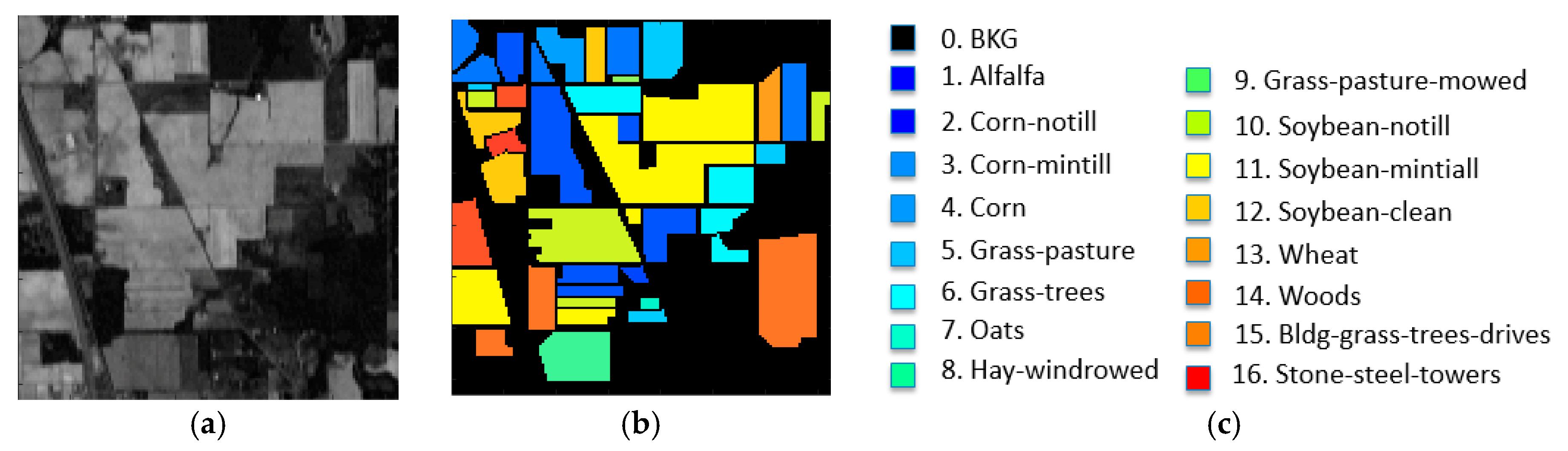
5.1. Purdue Indiana Indian Pines Scene

The first image scene used for experiments is an airborne visible/infrared imaging spectrometer (AVIRIS) hyperspectral data set from the Purdue Indiana Indian Pines test site shown in Figure 1a, with its ground truth of 17 class maps in Figure 1b. It has a size of $145\times 145$ pixel vectors, taken from an area of mixed agriculture and forestry in Northwestern Indiana, USA with details of band and wavelength given in the caption. The data set is available at website https://purr.purdue.edu/publications/1947/serve/1?el=1. It was recorded in June 1992 with 220 bands which include water absorption bands (bands 104–108 and 150–163, 220).

5.2. Salinas

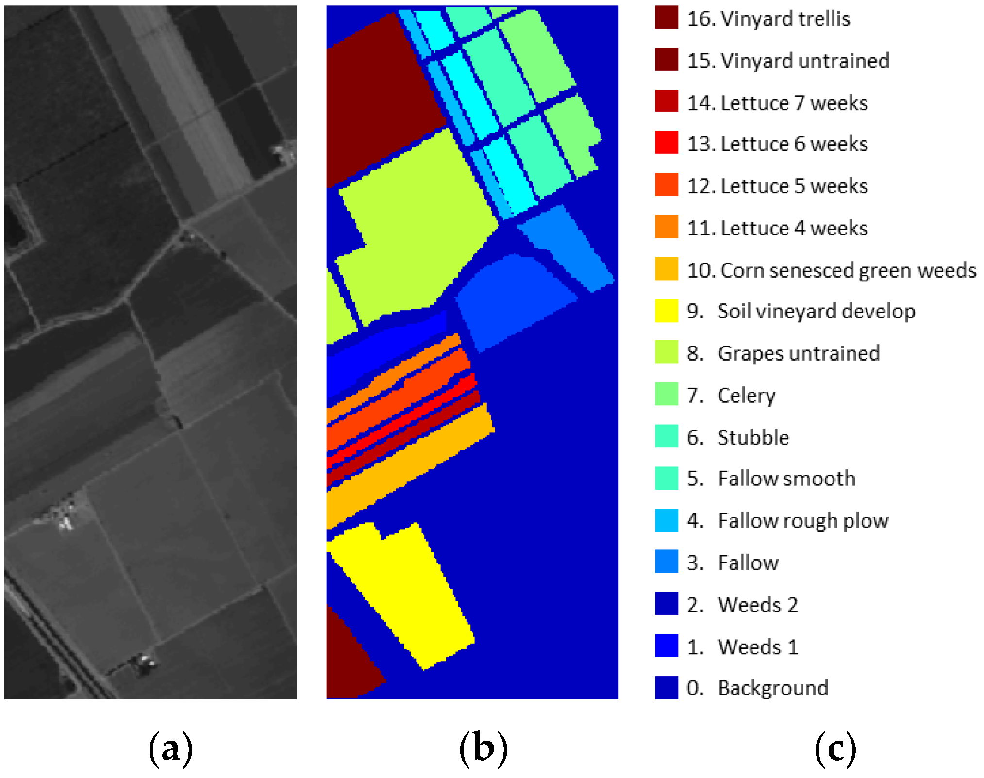
A second set of AVIRIS data used for experiments was the Salinas scene shown in Figure 2a, which was captured by the AVIRIS sensor over Salinas Valley, California, with a spatial resolution of 3.7 m per pixel and spectral resolution of 10 nm. It has a size of $512\times 217\times 224$. Figure 2b,c show the color composite of the Salinas image along with the corresponding ground truth class labels.

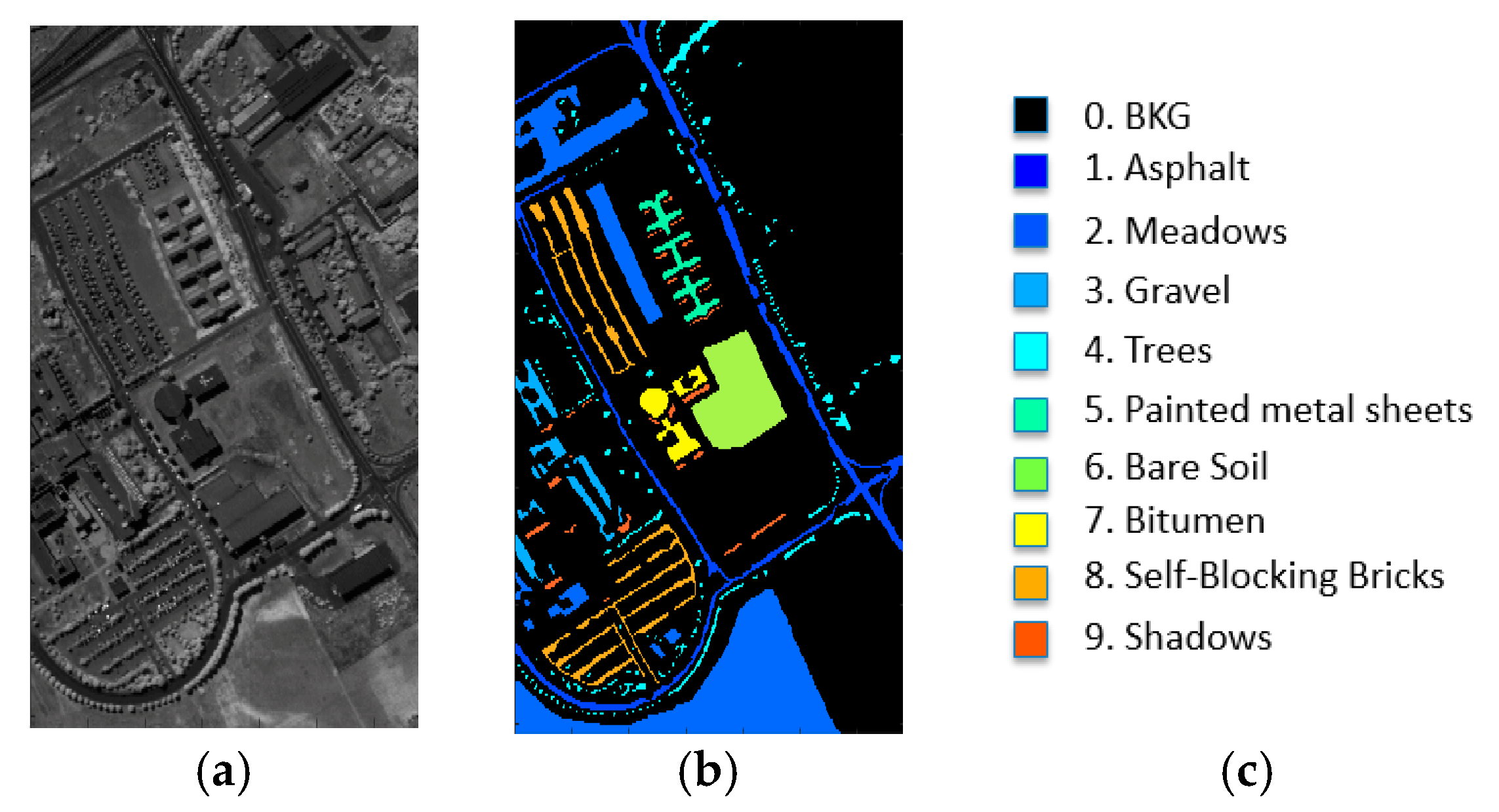
5.3. ROSIS Data

The last hyperspectral image data used for experiments was the University of Pavia image shown in Figure 3, which is an urban area surrounding the University of Pavia, Italy. It was recorded using the ROSIS-03 satellite sensor. It is of size $610\times 340\times 115$ with a spatial resolution of 1.3 m per pixel and spectral coverage ranging from 0.43 to 0.86 μm with spectral resolution of 4 nm (the 12 most noisy channels were removed before experiments). Nine classes of interest, plus a background (BKG) class (class 0), were considered for this image.

In the following experiments, four types of BS methods were tested for a comparative study and analysis.

• Uniform band selection (UBS): According to our extensive experiments, UBS is a reasonably good BS method which is also reported in the literature. It does not require any prior knowledge or BS criterion. It is the simplest BS method.
• MEAC: This uses the minimum covariance derived from the estimated abundance matrix, which is similar to the minimum variance in (5). In addition, it can also represent the category of SQMBS methods.
• MDPP and DSEBS: Both represent the category of SMMBS methods. They make use of graph representations to specify band groups. Most importantly, these two methods were compared with CEM/LCMV-based methods in [26] and both are also based on the LCMV formulation specified by (2).
• LCMV-BSS developed in this paper: This represents the category of BSS methods using the LCMV formulation in (2).

As noted in the introduction and in Section 3, although PSO, FA, and MTSP are also SMMBS methods, they are not compared in this paper for the following reasons. One is that their design rationale is completely different from that of LCMV-BSS. Secondly, the initial candidate sets from which their search algorithms find an optimal band subset are random and are also too small. So, their results are not representative and also are not reproducible. Thirdly, the details of their used parameters were not specified and provided in their papers. Therefore, it is very difficult to implement their algorithms for fair comparisons.

Table 1. n_BS estimated by HySime and HFC/NWHFC.

	PF = 10−1	PF = 10−2	PF = 10−3	PF = 10−4	PF = 10−5
Purdue	73/21	49/19	35/18	27/18	25/17
Salinas	32/33	28/24	25/21	21/21	20/20
Univ. of Pavia	25/34	21/27	16/17	14/14	13/12

tabulates the number n_BS of selected bands estimated for three scenes using Harsanyi-Farrand-Chang (HFC) method/noise whitened HFC (NWHFC method developed for VD in [69,74,75] where n_BS was determined to be n_BS = 18 for Purdue’s data, 21 for Salinas and 14 for University of Pavia with a false alarm probability of 10⁻⁴.

Table 2. Bands selected by UBS, SQ LCMV-BSS-1, SQ LCMV-BSS-2, SC LCMV-BSS.

Data	Methods	Selected Bands
Purdue Indian Pines (18 bands)	UBS	1, 14, 27, 40, 53, 66, 79, 92, 105, 118, 131, 144, 157, 170, 183, 196, 209, 220
	MEAC	159, 3, 92, 96, 82, 36, 39, 55, 41, 1, 2, 33, 206, 38, 163, 17, 204, 9
	MDPP	10, 39, 59, 75, 79, 85, 92, 130, 140, 146, 147, 149, 150, 152, 160, 164, 175, 193
	DSEBS	42, 129, 97, 131, 174, 16, 176, 177, 172, 43, 192, 193, 98, 171, 99, 132, 40, 33
	SQ LCMV-BSS-1	39, 164, 29, 155, 108, 66, 79, 8, 105, 42, 44, 17, 156, 150, 3, 43, 213, 41
	SQ LCMV-BSS-2	38, 109, 29, 52, 163, 66, 158, 8, 164, 219, 43, 78, 157, 220, 3, 49, 218, 2
	SC LCMV-BSS	54, 156, 42, 159, 53, 41, 79, 91, 105, 57, 51, 43, 157, 48, 107, 160, 115, 163
Salinas (21 bands)	UBS	1, 12, 23, 34, 45, 56, 67, 78, 89, 100, 111, 122, 133, 144, 155, 166, 177, 188, 199, 210, 224
	MEAC	107, 148, 203, 149, 5, 8, 105, 3, 28, 12, 18, 10, 44, 36, 25, 17, 51, 32, 110, 68, 58
	MDPP	1, 8, 11, 22, 27, 28, 50, 57, 58, 65, 90, 99, 105, 119, 123, 134, 142, 157, 175, 191, 204
	DSEBS	99, 101, 16, 119, 177, 112, 44, 46, 120, 47, 131, 175, 196, 121, 17, 102, 174, 180, 187, 135, 42
	SQ LCMV-BSS-1	7, 50, 23, 48, 45, 73, 65, 15, 40, 19, 80, 122, 38, 41, 42, 46, 78, 47, 200, 37, 2
	SQ LCMV-BSS-2	7, 42, 56, 28, 45, 58, 67, 15, 41, 19, 50, 122, 38, 34, 36, 47, 224, 46, 183, 37, 172
	SC LCMV-BSS	18, 39, 41, 31, 45, 44, 67, 78, 90, 101, 40, 91, 42, 141, 46, 48, 102, 185, 47, 86, 50
Univ. of Pavia (14 bands)	UBS	1, 9, 17, 25, 33, 41, 49, 57, 65, 73, 81, 89, 97, 103
	MEAC	1, 23, 24, 40, 42, 58, 56, 59, 48, 31, 47, 83, 25, 54
	MDPP	2, 23, 44, 46, 50, 62, 66, 73, 89, 91, 92, 93, 96, 102
	DSEBS	86, 102, 64, 20, 21, 63, 65, 6, 19, 22, 7, 66, 95, 67
	SQ LCMV-BSS-1	1, 4, 55, 16, 95, 83, 84, 93, 39, 77, 91, 102, 92, 103
	SQ LCMV-BSS-2	1, 4, 38, 76, 85, 55, 84, 102, 16, 83, 93, 89, 92, 103
	SC LCMV-BSS	1, 4, 84, 16, 38, 102, 85, 92, 83, 72, 95, 91, 96, 103

lists the bands selected by seven BS methods—uniform BS (UBS), minimum estimated abundance covariance (MEAC), multigraph determinantal point process (MDPP), dominant set extraction BS (DSEBS), SQ LCMV-BSS-1, SQ LCMV-BSS-2, and SC LCMV-BSS—for the three scenes; n_BS = 18 for Purdue’s Indian Pines, n_BS = 21 for Salinas, and n_BS = 14 for University of Pavia.

In order to perform HSIC, choosing an appropriate classifier is crucial. Recently, Yu et al. [76] developed a new classifier, called the iterative multiclass constrained background suppression classifier (IMCBSC), and further demonstrated that IMCBSC performed well in both overal accuarcy rate (P_OA) and precision rate (P_R) Since IMCBSC was also derived from LCMV and implemented by LCMV in an iterative manner, the iterative linearly constrained minimum variance (ILCMV) is used in this paper instead of IMCBSC to reflect its idea arising from LCMV and its iterative nature in algorithm implementation. Most importantly, ILCMV was adopted for two main reasons. One is because of the work in [76], which showed that ILCMV could perform at least comparably in P_OA but significantly better than the work in [12]. The other is that ILCMV is indeed derived from the LCMV criterion specified by (2). So, it is natural to use ILCMV to perform classification.

Two remarks on the implementation of ILCMV are noteworthy.

• Unlike most supervised classifiers used for HSIC which require training samples, ILCMV only needs the knowledge of the class signatures D, which can be obtained by either prior knowledge or class sample means. Specifically, the class signatures in D are not necessarily real data samples.
• Also, unlike most supervised classifiers used for HSIC which require test and training data samples from the same class, the test samples for ILCMV can be selected from any arbitrary class including the BKG class, and are not necessarily limited to the same class trained by the training samples. This is a crucial difference between ILCMV and existing hyperspectral image classification algorithms reported in the literature. For more details, we refer to [23,76].

Figure 4c–i, Figure 5c–i and Figure 6c–i show classification maps produced by ILCMV, using bands selected in Table 2 by seven BS methods—UBS, MEAC, MDPP, DSEBS, SQ LCMV-BSS-1, SQ LCMV-BSS-2, and SC LCMV-BSS, respectively—where the ground truth map and classification map produced by the full bands are also included in (a) and (b), respectively, for comparison.

Apparently, it is difficult to see any appreciable difference among all the classification results in Figure 4, Figure 5 and Figure 6 by visual inspection. In this case, to better evaluate each BS method, conducting a quantitative analysis is necessary. It has been shown in [23,76] that using overall accuracy (OA), P_OA may not be sufficient to evaluate the effectiveness of classification performance. To address this issue, two additional measures, called precision rate, P_R, and detection rate, P_D (also known as recall rate), developed in [23,76] were introduced for HSIC where P_R and P_D have been widely used in pattern recognition such as medical imaging, handwritten character recognition, and biometric recognition. The definitions and details of P_OA, P_R, and P_D can be found in [23,76].

Table 3. P_D, P_OA, and P_R calculated from the classification results in Figure 4 for Purdue’s data.

Class	Full Bands		UBS		MEAC		MDPP		DSEBS		SQ LCMV-BSS-1		SQ LCMV-BSS-2		SC LCMV-BSS
	PD	PR	PD	PR	PD	PR	PD	PR	PD	PR	PD	PR	PD	PR	PD	PR
1	95.65	100	95.65	100	93.48	100	95.65	100	95.65	100	95.65	100	97.83	100	100	100
2	96.01	100	97.13	99.57	93.07	99.63	96.08	100	96.99	100	95.59	99.71	93.78	99.85	94.89	99.85
3	96.99	99.88	96.51	100	96.27	100	97.35	100	97.23	99.88	96.39	100	95.67	100	94.10	100
4	98.73	100	98.73	100	98.31	100	99.58	100	98.31	100	97.89	100	98.31	100	98.31	100
5	89.44	100	90.68	100	91.51	100	92.34	100	93.58	100	91.93	100	92.34	100	92.96	100
6	97.12	100	97.67	100	97.40	99.58	96.71	100	97.12	100	96.44	100	97.95	100	95.75	100
7	100	100	100	100	100	100	100	100	100	100	100	100	100	100	100	100
8	98.78	100	98.54	100	99.16	100	97.49	100	97.91	100	97.91	100	99.16	100	98.95	100
9	100	100	100	100	90.00	100	100	100	100	100	100	90.91	100	95.24	100	100
10	93.93	99.78	91.98	100	93.31	100	94.65	99.78	93.00	100	94.24	100	91.98	99.58	91.98	100
11	94.70	99.87	96.13	99.96	94.55	98.22	95.48	99.87	95.85	100	95.48	99.96	96.17	100	95.93	99.49
12	95.45	100	94.94	100	96.29	100	96.80	100	97.30	100	95.95	100	95.11	100	96.63	100
13	98.54	100	98.54	100	99.02	100	97.56	100	96.59	100	97.56	100	98.54	100	98.54	100
14	93.52	100	94.15	100	94.78	100	94.70	100	94.55	100	95.89	100	96.05	100	96.13	100
15	90.67	100	95.60	100	92.49	100	96.89	100	93.52	100	94.82	100	94.56	100	96.11	100
16	98.92	98.92	98.92	98.92	98.92	100	98.92	98.92	98.92	100	98.92	100	97.85	100	95.70	97.80
POA	95.09		95.69		94.91		95.89		95.88		95.67		95.48		95.46
PR	97.61		97.90		97.52		98.00		97.99		97.89		97.80		97.79

,

Table 4. P_D, P_OA, and P_R calculated from the classification results in Figure 5 for Salinas.

Class	Full Bands		UBS		MEAC		MDPP		DSEBS		SQ LCMV-BSS-1		SQ LCMV-BSS-2		SC LCMV-BSS
	PD	PR	PD	PR	PD	PR	PD	PR	PD	PR	PD	PR	PD	PR	PD	PR
1	95.52	100	97.16	100	97.71	100	97.76	100	97.16	100	96.37	100	97.01	100	96.91	100
2	98.42	100	98.85	100	98.44	100	97.99	100	99.17	100	98.79	100	98.36	100	98.71	100
3	93.78	99.70	95.50	100	94.03	100	93.98	100	95.65	100	90.44	100	95.14	100	95.95	100
4	95.62	100	94.69	98.80	94.33	97.84	97.49	98.76	94.74	99.62	96.56	98.39	95.91	99.11	92.04	94.83
5	96.90	100	96.45	100	95.19	99.88	95.22	100	96.90	99.85	95.87	100	95.94	100	90.78	99.79
6	98.79	100	98.59	100	98.56	100	98.79	100	98.56	100	97.95	100	98.91	100	97.75	100
7	98.63	100	98.21	100	98.18	100	97.99	100	97.65	100	98.35	100	98.44	100	98.32	100
8	96.69	98.26	95.81	99.39	97.40	99.84	95.23	99.74	96.11	99.38	95.84	99.06	97.47	100	96.61	99.42
9	95.87	100	95.60	100	94.74	100	95.29	100	95.73	100	94.79	100	94.89	100	95.44	100
10	96.67	100	96.37	100	96.34	100	96.46	100	97.25	100	95.73	100	96.58	100	96.77	100
11	97.75	100	97.85	100	91.10	100	97.75	100	98.31	100	95.79	100	97.38	100	97.66	100
12	97.15	100	96.16	100	95.54	100	97.46	100	97.66	100	96.32	100	95.39	100	95.43	100
13	96.51	100	96.94	99.44	93.35	99.88	96.40	100	95.63	100	87.77	100	97.38	99.78	94.00	98.97
14	95.89	100	98.14	100	97.66	99.90	97.01	100	98.04	100	97.76	99.05	97.20	100	96.93	99.81
15	94.00	98.66	95.27	98.09	96.52	100	95.42	96.70	95.25	98.84	95.42	97.73	96.27	99.86	95.84	98.60
16	93.30	100	96.07	100	93.86	100	95.07	100	95.02	100	95.68	100	95.13	100	95.41	100
POA	96.37		96.49		96.45		96.25		96.63		95.93		96.81		96.21
PR	98.23		98.29		98.27		98.17		98.36		98.02		98.45		98.15

and

Table 5. P_D, P_OA, and P_R calculated from the classification results in Figure 6 for University of Pavia.

Class	Full Bands		UBS		MEAC		MDPP		DSEBS		SQ LCMV-BSS-1		SQ LCMV-BSS-2		SC LCMV-BSS
	PD	PR	PD	PR	PD	PR	PD	PR	PD	PR	PD	PR	PD	PR	PD	PR
1	86.42	99.90	87.67	99.45	86.44	99.76	87.97	99.68	87.71	99.74	84.44	99.63	88.05	99.44	88.67	99.77
2	73.34	99.99	84.38	99.95	83.33	99.89	82.14	99.96	84.63	99.92	84.14	99.89	85.21	99.98	86.76	99.95
3	79.85	96.30	78.90	100	76.66	100	76.17	99.02	79.22	100	76.49	100	74.71	100	78.56	99.95
4	98.81	96.65	97.84	95.16	98.88	87.91	96.95	91.85	97.99	88.71	98.14	88.96	97.77	95.30	97.70	93.11
5	91.49	100	89.93	100	91.33	100	93.32	100	87.11	100	93.50	100	90.57	100	90.77	100
6	89.10	99.98	91.35	100	82.78	100	87.53	100	87.44	100	86.19	100	90.00	100	91.13	100
7	81.10	100	83.32	100	76.26	100	75.64	100	76.34	100	82.84	100	82.92	100	82.46	100
8	78.46	85.20	79.09	97.37	79.51	97.20	79.83	95.71	79.30	97.44	77.09	97.16	77.09	98.45	79.30	98.96
9	77.24	99.87	75.86	99.47	76.32	100	74.01	98.44	76.17	100	80.21	99.46	78.22	99.86	77.08	99.87
POA	84.32		85.19		83.85		84.33		84.25		84.45		85.41		85.92
PR	96.76		96.93		96.64		96.76		96.75		96.78		96.96		96.95

show P_D, P_OA, and P_R calculated by the ILCMV classification results in Figure 4, Figure 5 and Figure 6 using the bands selected in Table 2 for Purdue’s data, Salinas, and University of Pavia, respectively, where the best results with highest rates are shown in boldface. Here, we would like to point out a crucial fact used in the experiments, as noted in the second remark described above, where the P_D, P_OA, and P_R were calculated by including the background (BKG) for classification because LCMV is particularly designed to take care of the BKG issue in classification, as shown in [76]. This is quite different from many reports which calculate P_OA excluding BKG from classification, such as [12].

Since P_D varies with each class, it is difficult to evaluate the overall classification performance. So, our analysis is conducted based on P_OA and P_R. As we can see from the tables, SQ LCMV-BSS-2 and SC LCMV-BSS outperformed all the other five BS methods in terms of P_OA and P_R for Salinas and University of Pavia scenes, but were slightly worse than MDPP in P_OA and DSEBS in P_R. Interestingly, both MDPP and DSEBS produced the best results in terms of P_OA and P_R respectively for the Purdue data. As also noted in Table 3, Table 4 and Table 5, the P_OA and P_R using full bands were generally not as good as those produced by most of the test BS methods, but also worse than that produced by UBS. These experiments showed that hyperspectral image classification can benefit greatly from the judicious selection of bands with appropriately determined n_BS.

Table 6. Computing time in seconds required by six test BS methods: MEAC, MDPP, DSEBS, SQ LCMV-BSS-1, SQ LCMV-BSS-2, SC LCMV-BSS.

	MEAC	MDPP	DSEBS	SQ LCMV-BSS-1	SQ LCMV-BSS-2	SC LCMV-BSS
Purdue	13.70	41.14	0.58	7.00	7.10	6.93
Salinas	83.64	44.66	5.27	43.43	46.63	43.55
University of Pavia	44.53	29.22	4.62	16.67	17.52	16.84

tabulates the computing times in seconds for each of six BS methods in a computer environment with a 1.6 GHz Intel Core i5 with OS X EI Capitan and 4 GB 1600 MHz DDR3; the software used to run experiments was Matlab_R2014b. Obviously, the best time was achieved by DSEBS, followed by SC LCMV-BSS and SQ LCMV-BSS. The worst time was achieved by MDPP for the Purdue data and MEAC for Salinas and University of Pavia.

As noted above, a classifier can also have a significant impact on BS, especially when BKG is included for consideration. A recent work [12] developed four edge preserving filtering (EPF)-based techniques—EPF-B-c, EPF-G-c, EPF-B-g, and EPF-G-g for HSIC—and also conducted a comprehensive comparative analysis to show that their methods indeed performed better than most recently developed spectral–spatial techniques. Therefore, in what follows, we conducted experiments to evaluate the performance of ILCMV in comparison with these four EPF-based techniques with BKG particularly included for classification. To see this, we also implemented these four EPF-based techniques with “B” and “G” used to specify bilateral filter and guided filter, respectively, and “g” and “c” indicate that the first principal component and color composite of the three principal components are used as reference images [12].

Table 7. P_OA and P_R calculated by the classification results using the bands selected by SQ LCMV-BSS-1 for the Purdue data.

Class	EPF-B-g with Full Bands	EPF-B-c with Full Bands	EPF-G-g with Full Bands	EPF-G-c with Full Bands	ILCMV with Full Bands	EPF-B-g-BS	EPF-B-c-BS	EPF-G-g-BS	EPF-G-c-BS	ILCMV-BS
1	100	100	97.83	100	95.65	100	100	100	100	95.65
2	76.47	87.82	80.60	82.98	96.01	74.79	90.76	71.99	79.90	95.59
3	93.49	83.98	79.64	65.42	96.99	63.37	75.66	84.10	72.77	96.39
4	99.16	100	100	96.20	98.73	100	100	100	97.89	97.89
5	93.79	94.00	97.10	94.82	89.44	89.86	97.52	96.07	94.41	91.93
6	100	99.59	99.59	99.45	97.12	98.22	99.86	99.73	99.32	96.44
7	92.86	92.86	96.43	96.43	100	92.86	64.29	92.86	89.29	100
8	100	100	100	100	98.78	100	100	100	100	97.91
9	80.00	65.00	100	100	100	65.00	95.00	65.00	10.00	100
10	90.53	91.46	87.14	93.00	93.93	75.31	73.97	84.88	76.54	94.24
11	90.67	92.67	86.27	88.88	94.70	78.98	70.79	64.73	80.94	95.48
12	98.31	96.46	93.93	92.07	95.45	47.55	42.50	79.76	57.67	95.95
13	99.02	99.51	99.51	99.51	98.54	100	100	100	100	97.56
14	97.71	97.00	97.87	98.26	93.52	94.86	94.86	87.67	92.57	95.89
15	100	100	99.74	82.90	90.67	95.85	96.37	95.85	97.41	94.82
16	97.85	100	100	100	98.92	98.92	100	98.92	97.85	98.92
POA	92.27	93.45	90.32	89.79	95.09	81.62	82.94	81.17	84.15	95.67
PR	44.98	44.56	44.03	43.77	97.61	39.79	40.43	39.86	41.02	97.89
Time(s)	196.58	200.84	194.09	200.87	25.37	31.27	36.77	31.14	36.16	37.25

,

Table 8. P_OA and P_R calculated by the classification results using full bands and the bands selected by SQ LCMV-BSS-2 for the Purdue data.

Class	EPF-B-g with Full Bands	EPF-B-c with Full Bands	EPF-G-g with Full Bands	EPF-G-c with Full Bands	ILCMV with Full Bands	EPF-B-g-BS	EPF-B-c-BS	EPF-G-g-BS	EPF-G-c-BS	ILCMV-BS
1	100	100	100	100	95.65	100	100	100	100	97.83
2	86.83	82.49	86.62	84.52	96.01	85.78	81.86	64.22	66.60	93.78
3	90.84	85.90	82.53	80.72	96.99	81.93	74.58	63.98	64.82	95.67
4	99.16	99.16	100	99.58	98.73	99.16	100	99.58	100	98.31
5	95.03	92.96	97.72	92.34	89.44	93.17	95.03	91.72	92.13	92.34
6	100	99.86	99.59	99.73	97.12	99.73	97.81	100	99.59	97.95
7	89.29	89.29	96.43	96.43	100	92.86	78.57	96.43	92.86	100
8	100	100	100	100	98.78	100	100	100	100	99.16
9	60.00	75.00	70.00	50.00	100	100	95.00	65.00	35.00	100
10	92.59	90.33	90.74	92.49	93.93	70.27	66.26	64.71	54.42	91.98
11	89.12	89.33	88.51	86.44	94.70	64.89	70.26	82.12	82.24	96.17
12	96.46	98.31	98.15	98.99	95.45	67.45	52.78	51.10	34.74	95.11
13	99.02	99.02	99.51	99.51	98.54	99.51	99.51	99.51	99.51	98.54
14	98.81	98.18	96.36	95.02	93.52	90.59	97.79	92.81	89.41	96.05
15	99.74	100	94.04	95.34	90.67	90.41	90.41	93.26	83.42	94.56
16	100	100	100	100	98.92	95.70	98.92	100	100	97.85
POA	93.37	92.17	92.10	90.96	95.09	81.49	81.28	80.01	77.66	95.48
PR	45.52	44.93	44.89	44.34	97.61	39.72	39.61	39.00	37.85	97.80
Time(s)	194.14	199.37	194.13	200.36	25.37	31.16	37.93	32.56	36.51	41.58

,

Table 9. P_OA and P_R calculated by the classification results using full bands and the bands selected by SC LCMV-BSS for the Purdue data.

Class	EPF-B-g with Full Bands	EPF-B-c with Full Bands	EPF-G-g with Full Bands	EPF-G-c with Full Bands	ILCMV with Full Bands	EPF-B-g-BS	EPF-B-c-BS	EPF-G-g-BS	EPF-G-c-BS	ILCMV-BS
1	100	100	100	97.83	95.65	100	97.83	97.83	100	100
2	83.26	83.26	83.05	78.92	96.01	48.25	42.09	48.74	39.92	94.89
3	79.16	69.64	80.48	66.87	96.99	62.05	55.18	60.36	44.10	94.10
4	100	98.31	100	99.58	98.73	100	100	100	99.58	98.31
5	93.79	93.17	95.86	93.79	89.44	91.93	94.00	93.58	93.79	92.96
6	99.73	99.73	98.08	99.32	97.12	99.32	99.45	94.93	99.45	95.75
7	96.43	92.86	96.43	89.29	100	85.71	71.43	92.86	64.29	100
8	100	99.79	100	100	98.78	100	100	99.79	100	98.95
9	20.00	75.00	75.00	65.00	100	20.00	45.00	35.00	0	100
10	75.31	84.16	84.47	89.61	93.93	59.05	48.97	47.22	49.90	91.98
11	91.65	91.00	87.98	91.73	94.70	76.25	78.09	70.22	72.87	95.93
12	96.29	92.07	96.12	97.47	95.45	70.83	60.20	44.86	58.85	96.63
13	99.51	99.51	99.51	99.51	98.54	100	100	100	100	98.54
14	92.89	98.34	96.36	96.68	93.52	98.34	93.04	97.23	97.39	96.13
15	100	100	98.19	99.48	90.67	93.26	89.12	79.27	67.36	96.11
16	100	100	100	100	98.92	100	100	93.55	95.70	95.70
POA	90.06	90.42	90.56	90.37	95.09	77.37	74.12	72.31	71.25	95.46
PR	43.90	44.08	44.15	44.05	97.61	37.72	36.13	35.25	34.73	97.79
Time(s)	187.76	203.60	195.20	201.21	25.37	32.01	38.78	31.92	38.07	42.73

,

Table 10. P_OA and P_R calculated by the classification results using full bands and the bands selected by SQ LCMV-BSS-1 in Table 2 for Salinas.

Class	EPF-B-g with Full Bands.	EPF-B-c with Full Bands	EPF-G-g with Full Bands	EPF-G-c with Full Bands	ILCMV with Full Bands	EPF-B-g-BS	EPF-B-c-BS	EPF-G-g-BS	EPF-G-c-BS	ILCMV-BS
1	100	100	100	100	95.52	100	99.75	100	100	96.37
2	100	100	100	100	98.42	99.97	100	99.97	100	98.79
3	100	100	100	100	93.78	100	100	100	100	90.44
4	100	100	100	99.93	95.62	99.93	99.86	99.93	100	96.56
5	99.37	99.25	98.69	99.25	96.90	98.92	98.95	98.92	98.95	95.87
6	100	100	100	100	98.79	99.97	99.97	99.97	99.97	97.95
7	100	99.92	100	100	98.63	99.66	99.72	99.66	99.83	98.35
8	90.92	90.40	89.26	90.61	96.69	87.11	91.94	87.11	91.70	95.84
9	99.98	100	99.97	99.97	95.87	99.58	100	99.58	99.97	94.79
10	96.95	98.08	98.60	98.51	96.67	96.19	98.57	96.19	98.60	95.73
11	99.91	99.91	99.91	100	97.75	99.91	99.91	99.91	99.81	95.79
12	100	100	100	100	97.15	100	100	100	100	96.32
13	99.89	99.56	99.02	99.89	96.51	98.47	99.13	98.47	99.56	87.77
14	99.91	99.25	99.63	100	95.89	98.97	99.35	98.97	98.04	97.76
15	89.01	85.65	85.65	87.08	94.00	90.66	82.21	90.66	85.99	95.42
16	99.83	100	99.45	99.83	93.30	99.67	100	99.67	100	95.68
POA	96.40	95.89	95.64	96.17	96.37	95.64	95.73	95.64	96.19	95.93
PR	46.97	46.26	46.95	46.85	98.23	46.60	46.64	46.60	46.86	98.02
Time(s)	1060.77	741.84	1082.51	1134.06	167.80	75.17	78.73	75.17	104.31	134.96

,

Table 11. P_OA and P_R calculated by the classification results using full bands and the bands selected by SQ LCMV-BSS-2 in Table 2 for Salinas.

Class	EPF-B-g with Full Bands	EPF-B-c with Full Bands	EPF-G-g with Full Bands	EPF-G-c with Full Bands	ILCMV with Full Bands	EPF-B-g-BS	EPF-B-c-BS	EPF-G-g-BS	EPF-G-c-BS	ILCMV-BS
1	100	100	100	100	95.52	100	100	100	100	97.01
2	100	100	100	100	98.42	100	100	100	99.97	98.36
3	100	100	100	100	93.78	100	100	99.95	100	95.14
4	100	100	100	99.78	95.62	100	99.93	100	100	95.91
5	99.48	98.95	98.58	99.14	96.90	98.66	98.73	99.14	98.84	95.94
6	100	100	100	100	98.79	99.95	100	100	100	98.91
7	100	99.89	100	99.89	98.63	99.92	99.97	99.89	99.80	98.44
8	88.63	91.98	87.90	90.86	96.69	87.84	89.50	90.61	91.86	97.47
9	99.90	99.98	99.95	100	95.87	99.97	99.94	99.60	100	94.89
10	97.56	98.90	97.04	97.50	96.67	99.33	99.51	99.21	98.29	96.58
11	100	99.91	99.91	99.72	97.75	100	99.91	99.72	100	97.38
12	100	100	100	100	97.15	100	100	100	100	95.39
13	99.24	99.89	98.80	99.13	96.51	99.02	100	98.36	99.13	97.38
14	99.91	99.91	99.91	99.25	95.89	100	100	99.91	99.35	97.20
15	88.66	85.43	94.25	91.43	94.00	79.35	93.04	83.94	86.13	96.27
16	99.94	100	99.61	99.50	93.30	100	100	100	100	95.13
POA	95.91	96.24	96.42	96.69	96.37	94.56	96.77	95.71	96.24	96.81
PR	46.73	46.89	46.97	47.11	98.23	46.07	47.15	46.63	46.89	98.45
Time(s)	1128.55	755.52	1050.34	722.76	167.80	73.49	101.80	71.57	98.16	159.26

,

Table 12. P_OA and P_R calculated by the classification results using full bands and the bands selected by SC LCMV-BSS in Table 2 for Salinas.

Class	EPF-B-g with Full Bands	EPF-B-c with Full Bands	EPF-G-g with Full Bands	EPF-G-c with Full Bands	ILCMV with Full Bands	EPF-B-g-BS	EPF-B-c-BS	EPF-G-g-BS	EPF-G-c-BS	ILCMV-BS
1	100	100	100	100	95.52	100	100	100	100	96.91
2	100	100	100	100	98.42	99.95	99.84	99.92	99.97	98.71
3	100	100	100	100	93.78	99.90	100	100	99.90	95.95
4	100	100	100	100	95.62	100	99.57	100	99.86	92.04
5	99.07	99.22	99.10	98.92	96.90	98.88	99.55	99.33	98.99	90.78
6	100	100	100	100	98.79	100	100	100	99.90	97.75
7	100	99.97	100	99.97	98.63	99.61	99.89	100	99.94	98.32
8	90.18	89.51	89.40	91.38	96.69	90.88	89.02	90.68	90.30	96.61
9	100	99.98	99.81	99.94	95.87	99.95	99.95	99.97	100	95.44
10	97.47	97.71	97.41	99.48	96.67	98.90	99.24	98.11	98.29	96.77
11	100	100	100	100	97.75	100	99.72	99.34	99.72	97.66
12	100	100	100	100	97.15	100	100	100	100	95.43
13	100	99.89	98.91	99.89	96.51	99.34	99.89	99.24	99.13	94.00
14	100	100	100	99.81	95.89	99.35	99.63	98.79	98.32	96.93
15	88.99	84.26	88.08	86.90	94.00	89.74	93.35	78.92	88.92	95.84
16	99.28	99.89	100	99.94	93.30	100	100	100	99.94	95.41
POA	96.25	95.52	95.95	96.34	96.37	96.50	96.70	95.02	96.26	96.21
PR	46.89	46.53	46.75	46.94	98.23	47.02	47.11	46.29	46.90	98.15
Time(s)	1139.99	1106.95	1154.78	1089.61	167.80	73.06	94.17	69.92	91.50	147.30

,

Table 13. P_OA and P_R calculated by the classification results using full bands and the bands selected by SQ LCMV-BSS-1 in Table 2 for University of Pavia.

Class	EPF-B-g with Full Bands	EPF-B-c with Full Bands	EPF-G-g with Full Bands	EPF-G-c with Full Bands	ILCMV with Full Bands	EPF-B-g-BS	EPF-B-c-BS	EPF-G-g-BS	EPF-G-c-BS	ILCMV-BS
1	98.04	98.04	98.08	97.81	77.24	96.15	92.47	96.34	97.29	80.21
2	98.66	99.39	97.79	98.28	86.42	94.31	94.84	97.39	98.06	84.44
3	91.09	93.52	95.00	94.33	73.34	92.62	94.81	95.57	95.33	84.14
4	93.47	95.27	92.92	98.01	79.85	97.52	97.45	97.00	96.87	76.49
5	100	100	100	99.85	98.81	100	100	100	100	98.14
6	99.98	100	100	100	91.49	99.64	98.15	99.64	100	93.50
7	100	99.32	99.92	99.77	89.10	99.92	99.32	99.40	100	86.19
8	99.02	99.00	97.80	99.78	81.10	95.60	96.22	96.41	96.28	82.84
9	100	100	100	100	78.46	100	99.89	100	100	77.09
POA	98.12	98.67	97.80	98.46	84.32	95.96	97.49	97.49	98.01	84.45
PR	20.24	20.35	20.17	20.31	96.76	19.79	19.71	20.11	20.21	96.82
Time(s)	225.93	265.79	232.05	252.50	401.08	51.16	83.46	52.90	78.32	1387.01

,

Table 14. P_OA and P_R calculated by the classification results using full bands and the bands selected by SQ LCMV-BSS-2 in Table 2 for University of Pavia.

Class	EPF-B-g with Full Bands	EPF-B-c with Full Bands	EPF-G-g with Full Bands	EPF-G-c with Full Bands	ILCMV with Full Bands	EPF-B-g-BS	EPF-B-c-BS	EPF-G-g-BS	EPF-G-c-BS	ILCMV-BS
1	94.89	97.80	97.84	98.21	77.24	95.43	95.96	88.76	92.01	78.22
2	98.58	97.63	99.25	98.01	86.42	96.43	94.88	92.59	93.13	88.05
3	94.90	93.57	92.57	95.19	73.34	92.19	92.47	95.52	93.62	85.21
4	95.63	94.97	93.02	98.83	79.85	98.69	96.02	98.37	98.47	74.71
5	100	100	100	99.85	98.81	100	100	100	100	97.77
6	100	100	100	100	91.49	100	99.52	99.72	99.94	90.57
7	100	100	99.40	99.77	89.10	100	99.92	100	100	90.00
8	96.93	98.89	98.94	98.48	81.10	93.97	94.70	95.22	93.56	82.92
9	100	100	100	100	78.46	100	100	100	100	77.09
POA	97.76	97.85	98.36	98.39	84.32	96.74	95.97	94.25	94.78	85.41
PR	20.16	20.18	20.29	20.29	96.76	19.95	19.79	19.44	19.55	96.94
Time(s)	219.10	249.76	226.85	238.81	401.08	48.52	82.95	53.53	79.05	971.56

and

Table 15. P_OA and P_R calculated by the classification results using full bands and the bands selected by SC LCMV-BSS in Table 2 for University of Pavia.

Class	EPF-B-g with Full Bands	EPF-B-c with Full Bands	EPF-G-g with Full Bands	EPF-G-c with Full Bands	ILCMV with Full Bands	EPF-B-g-BS	EPF-B-c-BS	EPF-G-g-BS	EPF-G-c-BS	ILCMV-BS
1	99.43	97.16	97.95	97.98	77.24	95.93	92.73	98.27	97.99	77.08
2	98.19	99.15	98.80	98.79	86.42	95.44	94.31	97.00	96.23	88.67
3	99.24	95.09	94.85	93.57	73.34	93.52	91.04	92.38	94.14	86.76
4	93.93	94.65	94.61	98.27	79.85	97.52	96.74	98.27	96.96	78.56
5	100	99.85	100	99.93	98.81	100	100	100	100	97.70
6	99.96	99.34	99.68	100	91.49	99.70	98.11	99.05	100	90.77
7	100	100	99.70	99.77	89.10	99.62	99.47	99.92	99.55	91.13
8	96.85	98.13	97.77	99.51	81.10	92.88	92.61	92.99	92.97	82.46
9	100	100	100	100	78.46	100	100	100	100	79.30
POA	98.37	98.32	98.28	98.67	84.32	96.22	94.85	97.21	96.92	85.92
PR	20.29	20.28	20.27	20.35	96.76	19.85	19.56	20.05	19.99	97.09
Time(s)	238.01	270.24	234.01	259.33	401.08	51.13	83.41	49.37	76.48	998.17

tabulate the results in terms of P_OA and P_R rates produced by the four EFP-based methods and ILCMV, all of which included BKG for classification and also used the bands selected in Table 2 to implement the three image scenes. Data for the Purdue image is shown in Table 7, Table 8 and Table 9 using bands selected by SQ LCMV-BSS-1, SQ LCMV-BSS-2, and SC LCMV-BSS; data for Salinas is shown in Table 10, Table 11 and Table 12 using bands selected by SQ LCMV-BSS-1, SQ LCMV-BSS-2, and SC LCMV-BSS; and data for University of Pavia is shown in Table 13, Table 14 and Table 15 using bands selected by SQ LCMV-BSS-1, SQ LCMV-BSS-2, and SC LCMV-BSS. In addition, their computing times in seconds are included in the tables for comparison.

Several interesting findings can be derived from the results in Table 7, Table 8, Table 9, Table 10, Table 11, Table 12, Table 13, Table 14 and Table 15.

• It is very obvious to note that BSS did improve ILCMV classification results. Such an improvement cannot be found in the four EPF-based methods, where the classification results of the four EPF-based methods using band subsets could only get worse compared with the results using full bands. This may be due to the fact that the four EPF-based methods used principal component analysis (PCA) to compress the original data in preprocessing which retains some crucial information provided by full bands.
• The precision rates produced by the four EPF-based methods were very low as also noted in [23,76]. However, ILCMV using bands selected by LCMV-BSS consistently performed very well in both P_OA and P_R.
• According to Table 7, Table 8 and Table 9, ILCMV performed slightly better than the four EPF-based methods in P_OA but significantly better in P_R for Purdue’s data and Salinas. The scene of the University of Pavia is interesting, as shown in Table 13, Table 14 and Table 15. The four EPF-based methods performed very well in P_OA but did very poorly in P_R with about only 20%. Furthermore, P_OA produced by ILCMV may not be as good as those produced by the four EPF-based methods (about 10% less) but the P_R produced by ILCMV were around 96% which is nearly 4.8 times better than the 20% produced by the four EPF-based methods. These experiments demonstrated that the BKG issue is critical in data analysis of the University of Pavia and cannot be ignored or discarded in data processing. Unfortunately, this BKG issue has never been investigated in the past.
• Unlike the four EPF-based methods, which performed well in P_OA but very poorly in P_R, ILCMV consistently performs well in both P_OA and P_R, and even better when it is implemented in conjunction with BSS—a case that the EPF-based methods actually failed, as shown in Table 7, Table 8, Table 9, Table 10, Table 11, Table 12, Table 13, Table 14 and Table 15.
• Last but not least, BS is heavily determined by three factors: the data to be processed, the BS method selected, and the classifier used. Unfortunately, most works on BS for hyperspectral image classification have been focused on the design and development of BS methods but very little has been reported on performance evaluation of different classifiers which use the same set of bands selected by a BS method. For example, as shown in Table 7, Table 8, Table 9, Table 10, Table 11, Table 12, Table 13, Table 14 and Table 15, if the four EPF methods were implemented by BS, their classification results could not be improved, but those of ILCMV could.
• It should be noted that P_D results are not included in Table 7, Table 8, Table 9, Table 10, Table 11, Table 12, Table 13, Table 14 and Table 15 due to two reasons. One is that the results of P_D using full bands are already available in [23,76]. The other is that EPF-based methods using partial bands did not perform better than their counterparts using full bands. So, it does not make sense to include their results in tables. Besides this, due to limited space, there is no need to include their results.

6. Conclusions

This paper developed an SMMBS method, called LCMV-BSS, which selects multiple bands as a band subset using LCMV to linearly constrain class signature vectors as a criterion to select an optimal band subset. It is completely different from existing BS methods, with the following contributions: (i) It is a BSS method particularly developed for HSIC; (ii) It is quite different from single band-constrained methods in [26] and multiple-band constrained methods in [68], by constraining multiple class signature vectors instead of multiple bands; (iii) It develops three numerical search algorithms to find optimal band subsets which are different from the graph-based approaches [40,43] used by other SMMBS methods; (iv) It is very simple to implement via (7) with no parameters needing to be tuned; (v) Most importantly, it shows that HSIC can be improved by BS provided that the number n_BS of selected bands and the set of n_BS bands are properly selected.

References

- Melgani, F.; Bruzzone, L. Classification of hyperspectral remote sensing images with support vector machines. IEEE Trans. Geosci. Remote Sens. 2004, 42, 1778–1790. [Google Scholar] [CrossRef]
- Benediktsson, J.A.; Palmason, J.A.; Sveinsson, J.R. Classification of hyperspectral data from urban areas based on extended morphological profiles. IEEE Trans. Geosci. Remote Sens. 2005, 43, 480–491. [Google Scholar] [CrossRef]
- Camps-Valls, G.; Bruzzone, L. Kernel-based methods for hyperspectral image classification. IEEE Trans. Geosci. Remote Sens. 2005, 43, 1351–1362. [Google Scholar] [CrossRef]
- Tarabalka, Y.; Benediktsson, J.A.; Chanussot, J. Spectral-spatial classification of hyperspectral imagery based on partitional clustering techniques. IEEE Trans. Geosci. Remote Sens. 2009, 47, 2973–2987. [Google Scholar] [CrossRef]
- Tarabalka, Y.; Fauvel, M.; Chanussot, J.; Benediktsson, J.A. SVM- and MRF-based method for accurate classification of hyperspectral images. IEEE Geosci. Remote Sens. Lett. 2010, 9, 736–740. [Google Scholar] [CrossRef]
- Li, J.; Bioucas-Dias, J.M.; Plaza, A. Semisupervised hyperspectral image segmentation using multinominal logistic regression model with active learning. IEEE Trans. Geosci. Remote Sens. 2010, 48, 4085–4098. [Google Scholar]
- Zhang, B.; Li, S.; Jia, X.; Gao, L.; Peng, M. Adpative hyperspectral Markov random field approach for classification of hyperspectral imagery. IEEE Geosci. Remote Sens. Lett. 2011, 8, 4085–4098. [Google Scholar] [CrossRef]
- Li, J.; Bioucas-Dias, J.M.; Plaza, A. Hyperspectral image segmentation using a new Bayesion approach with active learning. IEEE Trans. Geosci. Remote Sens. 2011, 49, 3947–3960. [Google Scholar] [CrossRef]
- Chen, Y.; Nasabardi, N.; Tran, T.D. Hyperspectral image segmentation using dictionary-based sparse representation. IEEE Trans. Geosci. Remote Sens. 2011, 49, 3973–3985. [Google Scholar] [CrossRef]
- Tarabalka, Y.; Fauvel, M.; Chanussot, J.; Benediktsson, J.A. Segmentation and classification of hyperspectral images using minimum spanning forest grown from automatically selected makers. IEEE Trans. Syst. Man Cybern. Part B Cybern. 2011, 40, 1267–1279. [Google Scholar] [CrossRef] [PubMed]
- Fauvel, M.; Tarabalka, Y.; Benediktsson, J.A.; Chanussot, J.; Tilton, J. Advances in spectral-spatial classification of hyperspectral images. Proc. IEEE 2013, 101, 652–675. [Google Scholar] [CrossRef]
- Kang, K.; Li, S.; Benediktsson, J.A. Spectral-spatial hyperspectral image classification with edge-preserving filtering. IEEE Trans. Geosci. Remote Sens. 2014, 52, 2666–2677. [Google Scholar] [CrossRef]
- Fu, W.; Li, S.; Fang, L.; Kang, X.; Benediktsson, J.A. Hyperspectral image classification via shape-adaptive joint sparse representation. IEEE J. Sel. Top. Appl. Earth Obs. Remote Sens. 2016, 9, 556–567. [Google Scholar] [CrossRef]
- Kang, K.; Li, S.; Fang, L.; Li, M.; Benediktsson, J.A. Extended random walker-based classification of hyperspectral images. IEEE Trans. Geosci. Remote Sens. 2015, 53, 144–153. [Google Scholar] [CrossRef]
- Lu, T.; Li, S.; Fang, L.; Bruzzone, L.; Benediktsson, J.A. Set-to-set distance-based spectral spatial classification of hyperspectral images. IEEE Trans. Geosci. Remote Sens. 2016, 54, 7122–7134. [Google Scholar] [CrossRef]
- Guo, X.; Huang, X.; Zhang, L.; Plaza, A.; Benedikisson, J.A. Support tensor machines for classification of hyperspectral remote sesning imagery. IEEE Trans. Geosci. Remote Sens. 2016, 54, 3248–3264. [Google Scholar] [CrossRef]
- Ma, X.; Wang, H.; Wang, J. Semisupervised classification of hyperspectral image based on multi- decision labeling and deep feature learning. ISPRS J. Photogramm. Remote Sens. 2016, 120, 99–107. [Google Scholar] [CrossRef]
- Camps-Valls, G.; Gomez-Chova, L.; Munoz-Mari, J.; Vila-Frances, J.; Calpe-Maravilla, J. CKs for hyperspectral image classification. IEEE Geosci. Remote Sens. Lett. 2006, 3, 93–97. [Google Scholar] [CrossRef]
- Gurram, P.; Kwon, H. Contextual SVM using Hilbert space embedding for hyperspectral classification. IEEE Geosci. Remote Sens. Lett. 2013, 10, 1031–1035. [Google Scholar] [CrossRef]
- Peng, J.; Zhou, Y.; Chen, C. Region-kernel-based support vector machines for hyperspectral image classification. IEEE Trans. Geosci. Remote Sens. 2015, 53, 4810–4824. [Google Scholar] [CrossRef]
- Sun, S.; Zhong, P.; Xiao, H.; Wang, R. Active learning with Gaussian process classifier for hyperspectral image classification. IEEE Trans. Geosci. Remote Sens. 2015, 53, 1746–1760. [Google Scholar] [CrossRef]
- Pullanagari, R.; Kereszturi, G.; Yule, I.J.; Ghamisi, P. Assessing the performance of multiple spectral-spatial features of a hyperspectral image for classification of urban land cover classes using support vector machines and artificial neural network. J. Appl. Remote Sens. 2017, 11, 026009-1–026009-21. [Google Scholar] [CrossRef]
- Xue, B.; Yu, C.; Wang, Y.; Song, M.; Li, S.; Wang, L.; Chen, H.M.; Chang, C.-I. A subpixel target detection approach to hyperpsectral image classification. IEEE Trans. Geosci. Remote Sens. 2017, 55, 5093–5114. [Google Scholar] [CrossRef]
- Chang, C.-I. Hyperspectral Data Processing: Signal Processing Algorithm Design and Analysis; Wiley: Hoboken, NJ, USA, 2013. [Google Scholar]
- Chang, C.-I.; Du, Q.; Sun, T.S.; Althouse, M.L.G. A joint band prioritization and band decorrelation approach to band selection for hyperspectral image classification. IEEE Trans. Geosci. Remote Sens. 1999, 37, 2631–2641. [Google Scholar] [CrossRef]
- Chang, C.-I.; Wang, S. Constrained band selection for hyperspectral imagery. IEEE Trans. Geosci. Remote Sens. 2006, 44, 1575–1585. [Google Scholar] [CrossRef]
- Huang, R.; He, M. Band selection based on feature weighting for classification of hyperspectral data. IEEE Trans. Geosci. Remote Sens. Lett. 2005, 2, 156–159. [Google Scholar] [CrossRef]
- Keshava, N. Distance metrics and band selection in hyperspectral processing with applications to material identification. IEEE Trans. Geosci. Remote Sens. 2004, 42, 1552–1565. [Google Scholar] [CrossRef]
- Mausel, P.W.; Kramber, W.J.; Lee, J.K. Optimum band selection for supervised classification of multispectral data. Photogramm. Eng. Remote Sens. 1990, 56, 55–60. [Google Scholar]
- Jia, S.; Ji, Z.; Qian, Y.-Y.; Shen, L.-L. Unsupervised band selection for hyperspectral imagery classification without manual band removal. IEEE J. Sel. Top. Appl. Earth Obs. Remote Sens. 2012, 5, 531–543. [Google Scholar] [CrossRef]
- Stearns, S.D.; Wilson, B.E.; Peterson, J.R. Dimensionality reduction by optimal band selection for pixel classification of hyperspectral imagery. Proc. SPIE 1993, 2028, 118–127. [Google Scholar]
- Backer, S.; Kempeneers, P.; Debruyn, W.; Scheunders, P. Band selection for hyperspectral remote sensing. Pattern Recognit. 2005, 2, 319–323. [Google Scholar]
- Du, Q.; Yang, H. Similarity-based unsupervised band selection for hyperspectral image analysis. IEEE Geosci. Remote Sens. Lett. 2008, 5, 564–568. [Google Scholar] [CrossRef]
- Yang, H.; Du, Q. An efficient method for supervised hyperspectral band selection. IEEE Geosci. Remote Sens. Lett. 2011, 8, 138–142. [Google Scholar] [CrossRef]
- Su, H.; Du, Q.; Chen, G.; Du, P. Optimized hyperspectral band selection using particle swarm optimization. IEEE J. Sel. Top. Appl. Earth Obs. Remote Sens. 2014, 7, 2659–2670. [Google Scholar] [CrossRef]
- Su, H.; Yang, B.; Du, Q. Hyperspectral band selection using improved firefly algorithm. IEEE Geosci. Remote Sens. Lett. 2016, 13, 68–72. [Google Scholar] [CrossRef]
- Wei, W.; Du, Q.; Younan, N.H. Fast supervised hyperspectral band selection using graphics processing unit. J. Appl. Remote Sens. 2012, 6, 061504-1–061504-12. [Google Scholar]
- Yuan, Y.; Zhu, G.; Wang, Q. Hyperspectral band selection by multitask sparisty pursuit. IEEE Trans. Geosci. Remote Sens. 2015, 53, 631–644. [Google Scholar] [CrossRef]
- Lu, X.; Li, X.; Mou, L. Semi-supervised multitask learning for scene recognition. IEEE Trans. Cybern. 2015, 45, 1967–1976. [Google Scholar] [PubMed]
- Zhu, G.; Huang, H.; Lei, J.; Bi, Z.; Xu, F. Unsupervised hyperspectral band selection by dominant set extraction. IEEE Trans. Geosci. Remote Sens. 2016, 54, 227–239. [Google Scholar] [CrossRef]
- Yuan, Y.; Lin, J.; Wang, Q. Dual-clustering-based hyperspectral band selection by contextual analysis. IEEE Trans. Geosci. Remote Sens. 2016, 54, 1431–1445. [Google Scholar] [CrossRef]
- Wang, Q.; Lin, J.; Yuan, Y. Salient band selection for hyperspectral image classification via manifold ranking. IEEE Trans. Neural Netw. Learn. Syst. 2016, 27, 1279–1289. [Google Scholar] [CrossRef] [PubMed]
- Yuan, Y.; Zheng, X.; Lu, X. Discovering diverse subset for unsupervised hyperspectral band selection. IEEE Trans. Image Process. 2017, 26, 51–64. [Google Scholar] [CrossRef] [PubMed]
- Lu, X.; Yuan, Y.; Zheng, X. Joint dictionary learning for multispectral change detection. IEEE Trans. Cybern. 2017, 47, 884–897. [Google Scholar] [CrossRef] [PubMed]
- Lu, X.; Zheng, X.; Yuan, Y. Remote sensing scene classification by unsupervised representation learning. IEEE Trans. Geosci. Remote Sens. 2017, 55, 5148–5157. [Google Scholar] [CrossRef]
- Feng, J.; Jiao, L.C.; Zhang, X.; Sun, T. Hyperspectral band selection based on trivariate mutual information and clonal selection. IEEE Trans. Geosci. Remote Sens. 2014, 52, 4092–4105. [Google Scholar] [CrossRef]
- Feng, J.; Jiao, L.C.; Liu, F.; Sun, T.; Zhang, X. Mutual-information0-based semi-supervised hyperspectral band selection with high discrimination, high information and low redundancy. IEEE Trans. Geosci. Remote Sens. 2015, 53, 2956–2969. [Google Scholar] [CrossRef]
- Wang, C.; Gong, M.; Zhang, M.; Chan, Y. Unsupervised hyperspectral image band selection via column subset selection. IEEE Geosci. Remote Sens. Lett. 2015, 12, 1411–1415. [Google Scholar] [CrossRef]
- Geng, X.; Sun, K.; Ji, L. Band selection for target detection in hyperspectral imagery using sparse CEM. Remote Sens. Lett. 2014, 5, 1022–1031. [Google Scholar] [CrossRef]
- Sun, K.; Geng, X.; Ji, L. A new sparsity-based band selection method for target detection of hyperspectral image. IEEE Geosci. Remote Sens. Lett. 2015, 12, 329–333. [Google Scholar]
- Zare, A.; Gader, P. Hyperspectral band selection and endmember detection using sparisty promoting priors. IEEE Geosci. Remote Sens. Lett. 2008, 5, 256–260. [Google Scholar] [CrossRef]
- Ball, J.E.; Bruce, L.E.; Younan, N.H. Hyperspectral pixel unmixing via spectral band selection and DC-insensitive singular value decomposition. IEEE Geosci. Remote Sens. Lett. 2007, 4, 382–386. [Google Scholar] [CrossRef]
- Sun, K.; Geng, X.; Ji, L.; Lu, Y. A new band selection method for hyperspectral image based on data quality. IEEE J. Sel. Top. Appl. Earth Obs. Remote Sens. 2014, 7, 2697–2703. [Google Scholar]
- Sun, K.; Geng, X.; Ji, L. Exemplar component analysis: A fast band selection method for hyperspectral imagery. IEEE Geosci. Remote Sens. Lett. 2015, 12, 998–1002. [Google Scholar]
- Koonsanit, K.; Jaruskulchai, C.; Eiumnoh, A. Band selection for dimension reduction in hyper spectral image using integrated information gain and principal components analysis technique. Int. J. Mach. Learn. Comput. 2012, 2, 248–251. [Google Scholar] [CrossRef]
- Xia, W.; Wang, B.; Zhang, L. Band selection for hyperspectral imagery: A new approach based on complex networks. IEEE Geosci. Remote Sens. Lett. 2013, 10, 1229–1233. [Google Scholar] [CrossRef]
- Chang, C.-I.; Liu, K.-H. Progressive band selection for hyperspectral imagery. IEEE Trans. Geosci. Remote Sens. 2014, 52, 2002–2017. [Google Scholar] [CrossRef]
- Martínez-Usó, A.; Pla, F.; Sotoca, J.M.; García-Sevilla, P. Clustering-based hyperspectral band selection using information measures. IEEE Trans. Geosci. Remote Sens. 2007, 45, 4158–4171. [Google Scholar] [CrossRef]
- Yang, H.; Du, Q.; Sheng, Y. Semisupervised band clustering for dimensionality reduction of hyperspectral imagery. IEEE Geosci. Remote Sens. Lett. 2011, 8, 1135–1139. [Google Scholar]
- Su, H.; Du, Q. Hyperspectral band clustering and band selection for urban land cover classification. Geocarto Int. 2012, 27, 395–411. [Google Scholar] [CrossRef]
- Winter, M.E. N-finder: An algorithm for fast autonomous spectral endmember determination in hyperspectral data. Proc. SPIE 1999, 3753, 266–277. [Google Scholar]
- Wu, C.-C.; Chu, S.; Chang, C.-I. Sequential N-FINDR algorithm. In Proceedings of the SPIE Conference on Imaging Spectrometry XIII, San Diego, CA, USA, 10–14 August 2008. [Google Scholar]
- Xiong, X.; Wu, C.-C.; Chang, C.-I.; Kapalkis, K.; Chen, H.M. Fast algorithms to implement N-FINDR for hyperspectral endmember extraction. IEEE J. Sel. Top. Appl. Earth Obs. Remote Sens. 2011, 4, 545–564. [Google Scholar] [CrossRef]
- Chang, C.-I. Maximum Simplex Volume-Based Endmember Extraction Algorithms. U.S. Patent 8,417,748 B2, 9 April 2013. [Google Scholar]
- Chang, C.-I. Real Time Progressive Hyperspectral Image Processing: Endmember Finding and Anomaly Detection; Springer: New York, NY, USA, 2016. [Google Scholar]
- Wang, L.; Chang, C.-I.; Wang, Y.; Xue, B.; Song, M.; Yu, C.; Li, S. Band subset selection for anomaly detection in hyperspectral imagery. IEEE Trans. Geosci. Remote Sens. 2017, 55, 4887–4898. [Google Scholar] [CrossRef]
- Chang, C.-I.; Lee, L.C.; Xue, B.; Song, M.; Chen, J. Channel capacity approach to band subset selection for hyperspectral imagery. IEEE J. Sel. Top. Appl. Earth Obs. Remote Sens. 2017, 10, 4630–4644. [Google Scholar] [CrossRef]
- Wang, L.; Li, H.C.; Xue, B.; Chang, C.-I. Constrained band subset selection for hyperspectral imagery. IEEE Geosci. Remote Sens. Lett. 2017, 14, 2032–2036. [Google Scholar] [CrossRef]
- Chang, C.-I. Hyperspectral Imaging: Techniques for Spectral Detection and Classification; Kluwer Academic/Plenum Publishers: New York, NY, USA, 2003. [Google Scholar]
- Frost, O.L., III. An algorithm for linearly constrained adaptive array processing. Proc. IEEE 1972, 60, 926–935. [Google Scholar] [CrossRef]
- Chang, C.-I. Target signature-constrained mixed pixel classification for hyperspectral imagery. IEEE Trans. Geosci. Remote Sens. 2002, 40, 1065–1081. [Google Scholar] [CrossRef]
- Harsanyi, J.C. Detection and Classification of Subpixel Spectral Signatures in Hyperspectral Image Sequences; Department of Electrical Engineering, University of Maryland: Baltimore County, MD, USA, 1993. [Google Scholar]
- Pudil, P.; Novovicova, J.; Kittler, J. Floating search methods in feature selection. Pattern Recognit. Lett. 1994, 15, 1119–1125. [Google Scholar] [CrossRef]
- Chang, C.-I.; Du, Q. Estimation of number of spectrally distinct signal sources in hyperspectral imagery. IEEE Trans. Geosci. Remote Sens. 2004, 42, 608–619. [Google Scholar] [CrossRef]
- Harsanyi, J.C.; Farrand, W.; Chang, C.-I. Detection of subpixel spectral signatures in hyperspectral image sequences. In Proceedings of the American Congress on Surveying & Mapping (ACSM)/American Society of Photogrammetry & Remote Sensing (ASPRS) Annual Converntion and Exposition, Baltimore, MD, USA, 25–28 April 1994; Volume 1, pp. 236–247. [Google Scholar]
- Yu, C.; Xue, B.; Wang, Y.; Song, M.; Wang, L.; Li, S.; Chang, C.-I. Multi-class constrained background suppression approach to hyperspectral image classification. In Proceedings of the 2017 IEEE/GRSS International Geoscience and Remote Sensing Symposium (IGARSS), Fort Worth, TX, USA, 23–28 July 2017. [Google Scholar]