Fine-Resolution Precipitation Mapping in a Mountainous Watershed: Geostatistical Downscaling of TRMM Products Based on Environmental Variables


Abstract
:
1. Introduction
2. Materials and Methods
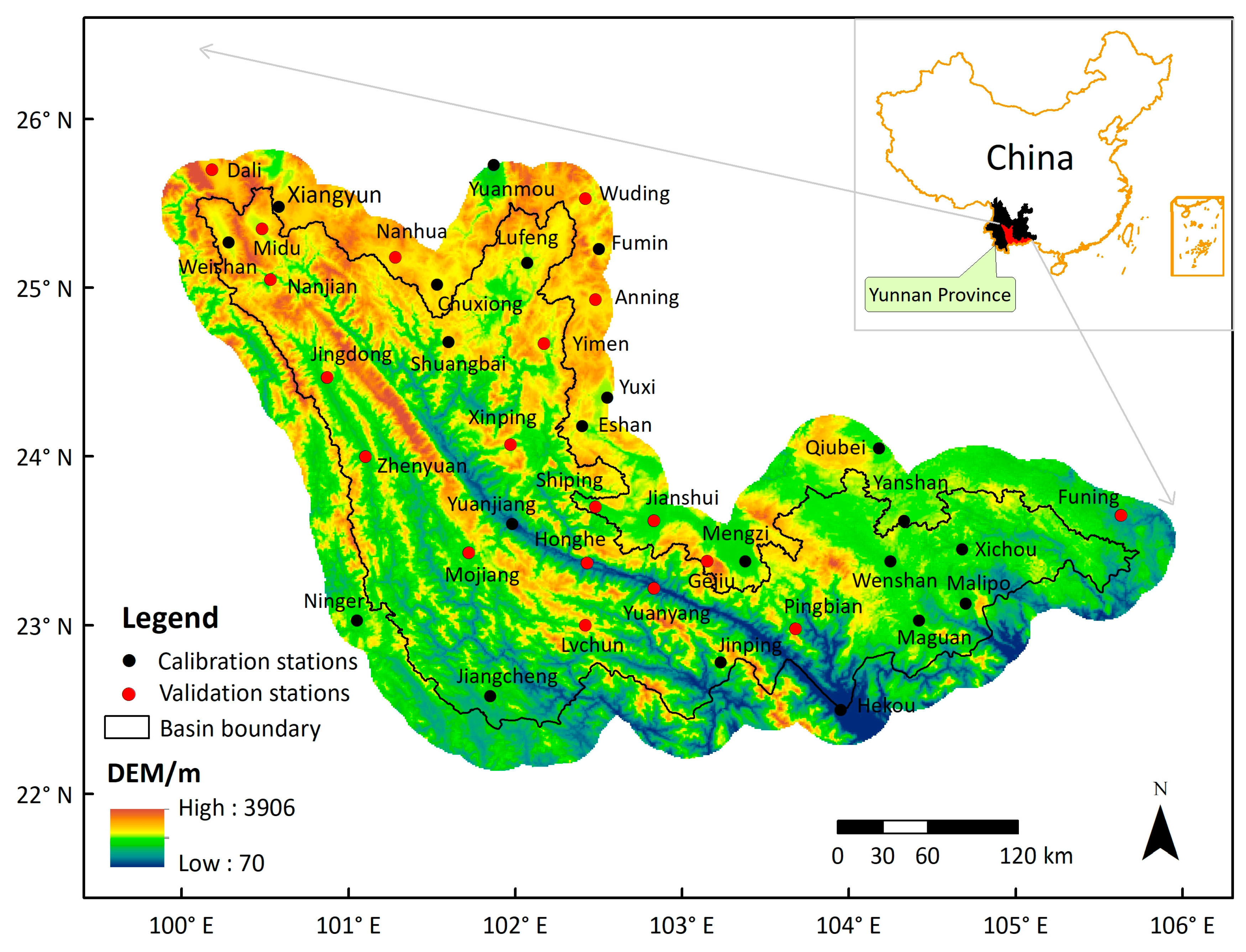
2.1. Study Area
2.2. Data
2.2.1. TRMM Precipitation Data
2.2.2. NDVI Data
2.2.3. Land Use Data
2.2.4. DEM Data
2.2.5. Rain Gauge Data
2.3. Methods
2.3.1. Downscaling of Original TRMM 3B43 Precipitation
2.3.2. Regression Models
2.3.3. Calibration of Downscaled Precipitation
- (1)
- The differences/ratio between the downscaled precipitation values and the measurements from RGS were computed;
- (2)
- The differences/ratio were interpolated into a resolution of 1-km with the interpolation technique; and
- (3)
- The downscaled precipitation was corrected to obtain the final calibrated precipitation by adding/multiplying the differences/ratio term of 1-km resolution.
2.3.4. Monthly Fraction Disaggregation from Annual Precipitation
- (1)
- The monthly fractions of 0.25°, which were used to disaggregate the annual precipitation, were defined as:where the represents the precipitation that occurs during the ith month as estimated from the original TRMM 3B43 product; and the denominator is the annual total value.
- (2)
- The 0.25° fractions were further interpolated into a spatial resolution of 1-km which was consistent with the downscaled-calibrated annual precipitation using an interpolation method;
- (3)
- The annual downscaled precipitation values at 1-km resolution were disaggregated into monthly-downscaled precipitation values by multiplying the fraction values of 1-km resolution.
2.3.5. Validation
3. Results
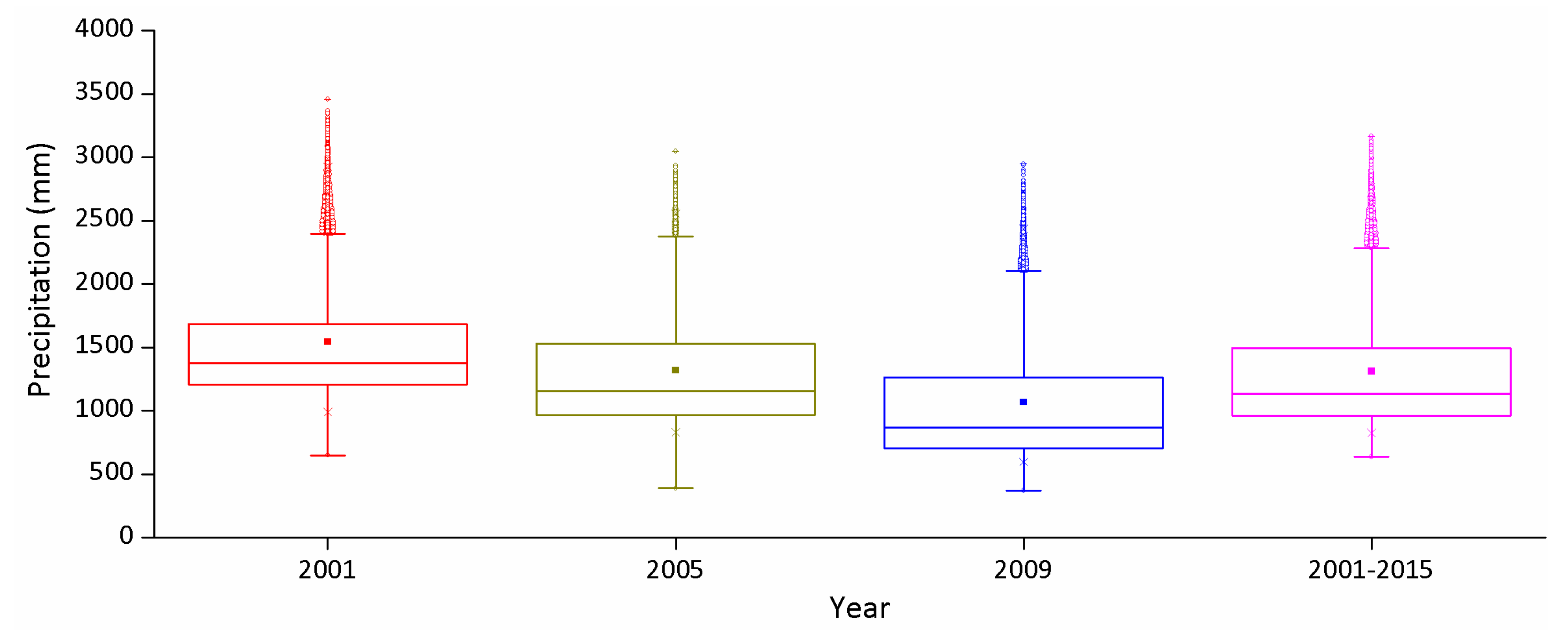
3.1. Comparison between TRMM and Station-Based Observed Precipitation
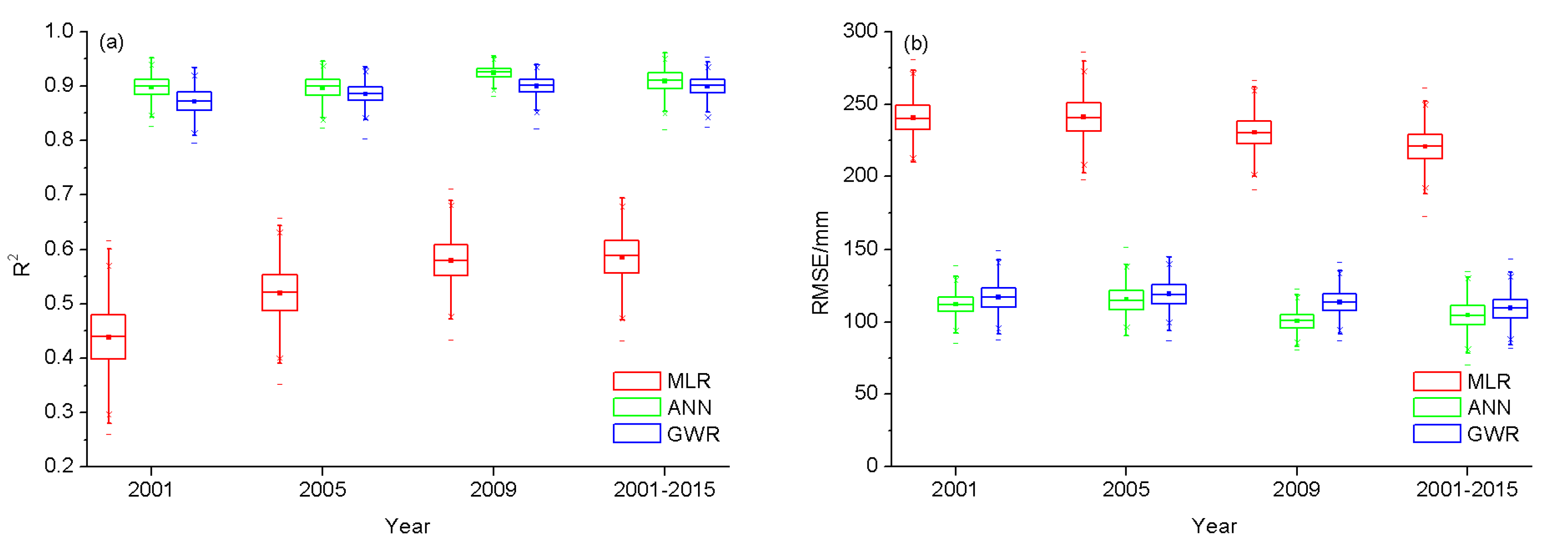
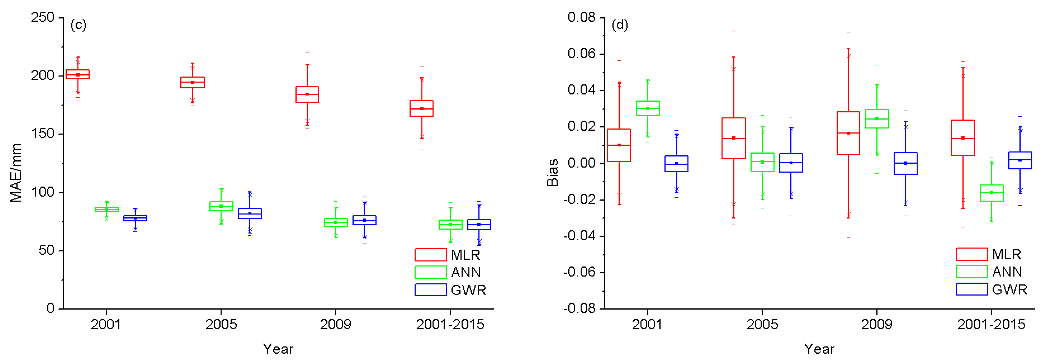
3.2. Performance of the Different Downscaling Models
3.3. Downscaling and Calibrating of TRMM Annual Precipitation
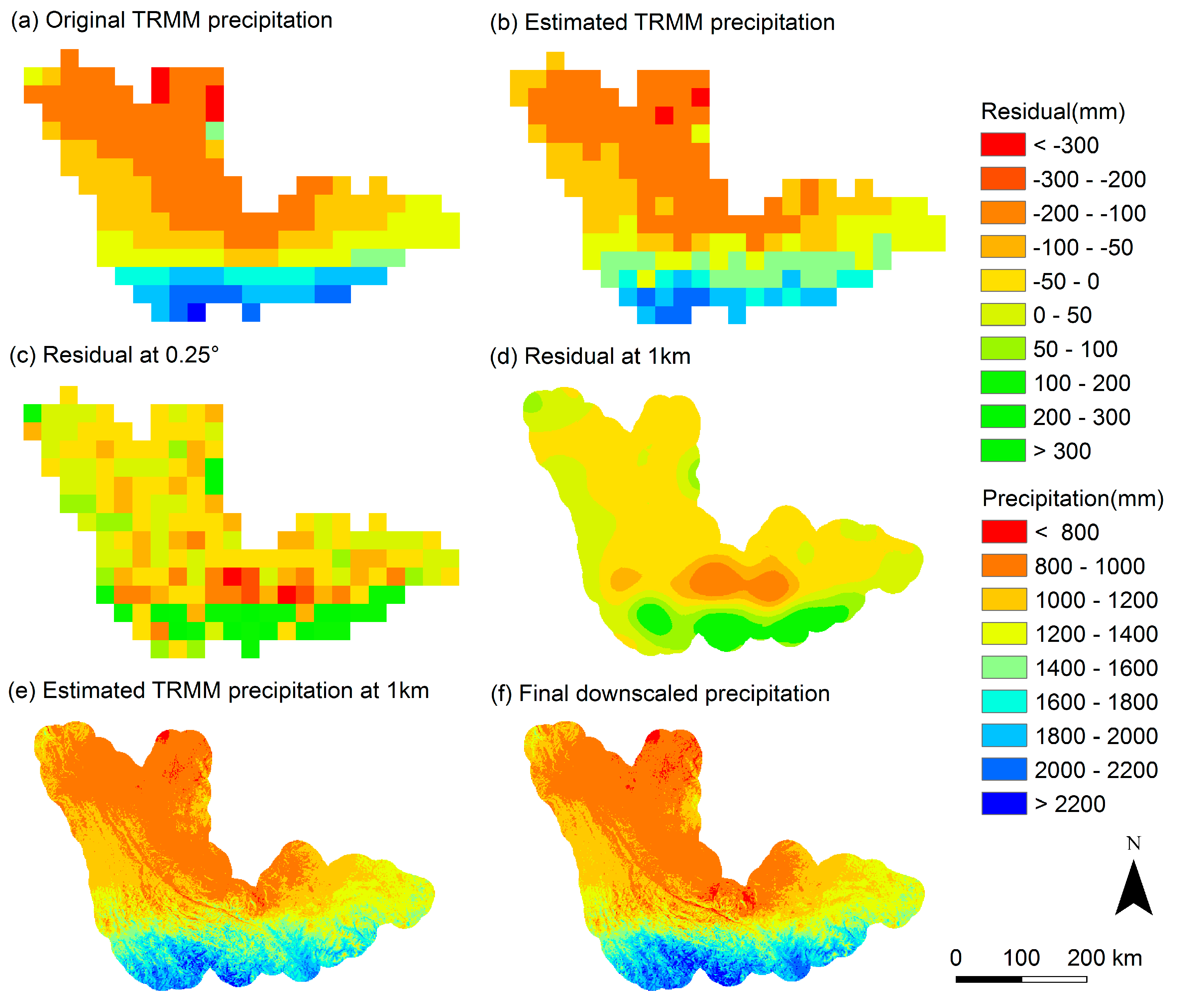
3.3.1. Downscaling Analysis of TRMM Annual Precipitation
3.3.2. Calibrating Analysis of Downscaled TRMM Annual Precipitation
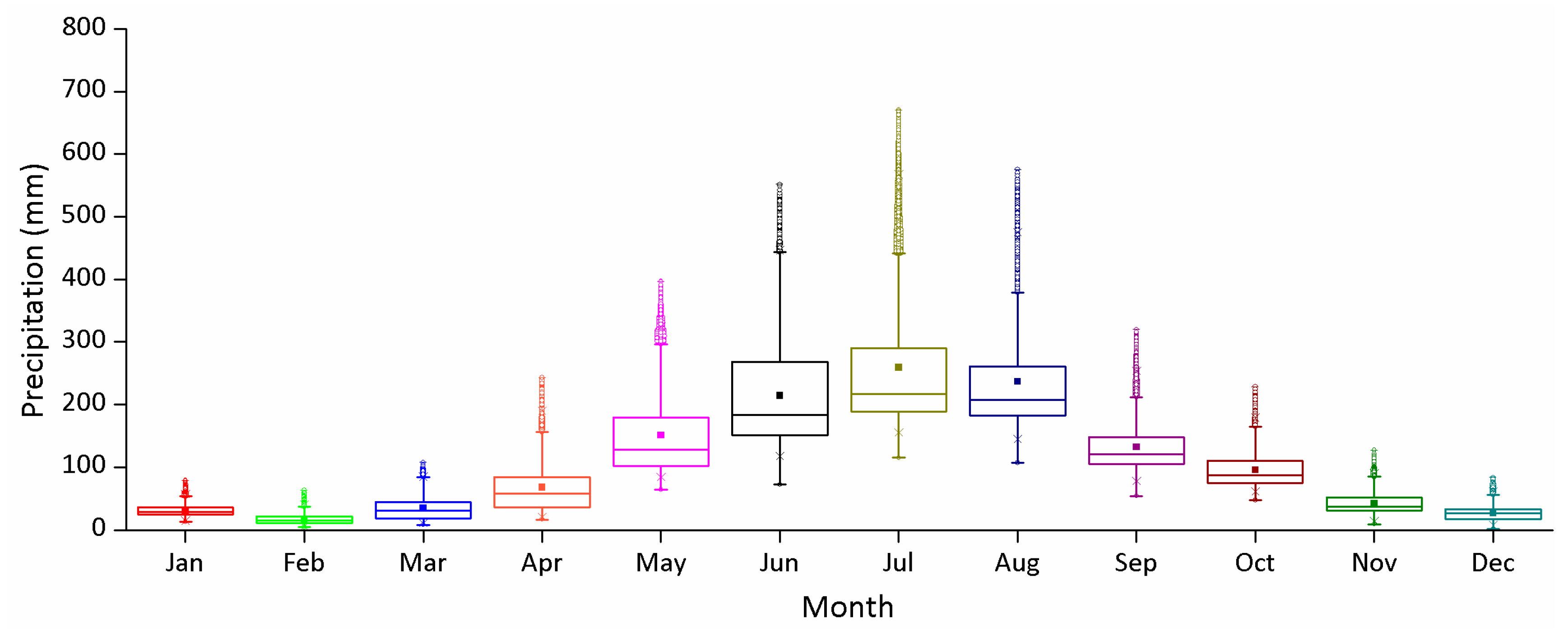
3.4. Monthly Results of Disaggregating Annual Precipitation
4. Discussion
4.1. Sources of Errors and Limitations in the Downscaled Satellite Precipitation Datasets
4.2. Precipitation-NDVI Relationships and Precipitation-Topography Relationships
4.3. The Downscaling Procedure
5. Conclusions
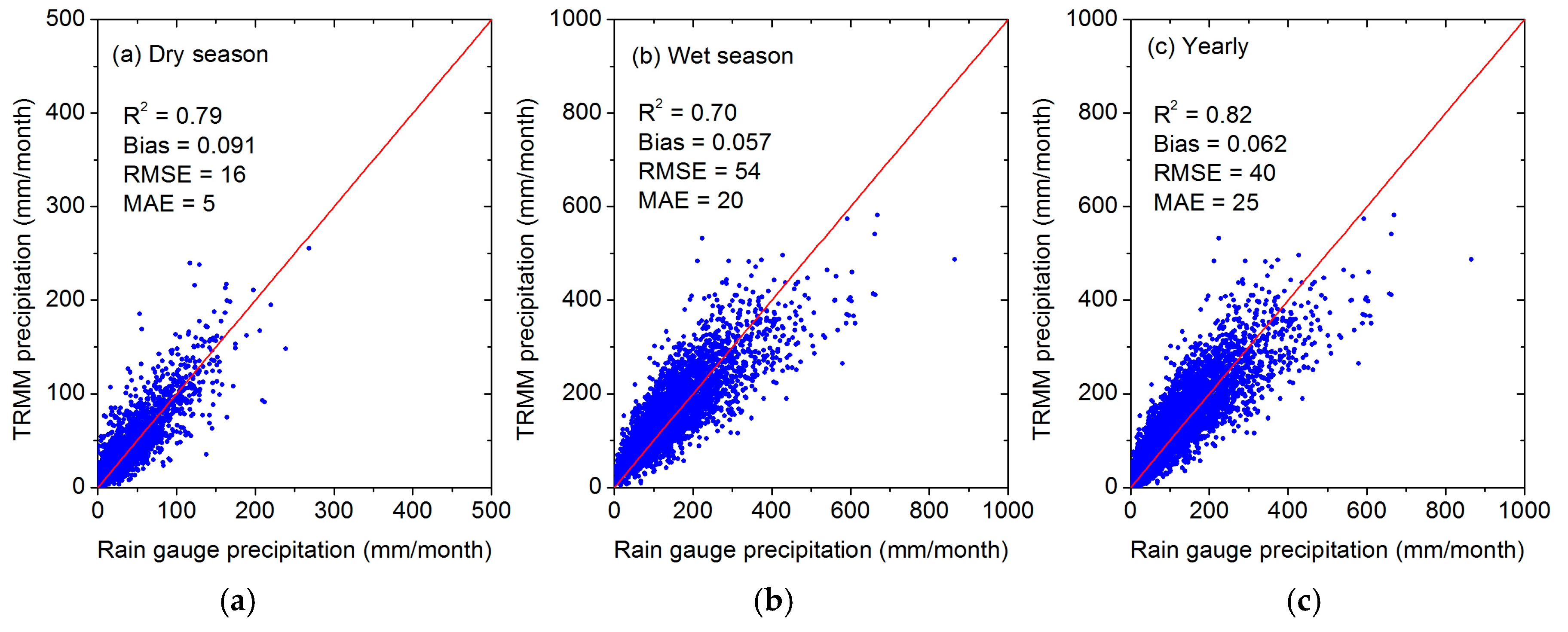
- A comparison between the TRMM precipitation and measurements from RGS indicated that good agreement was found between the two datasets. Moreover, TRMM precipitation was 6.2% higher than observations from RGS at a yearly scale.
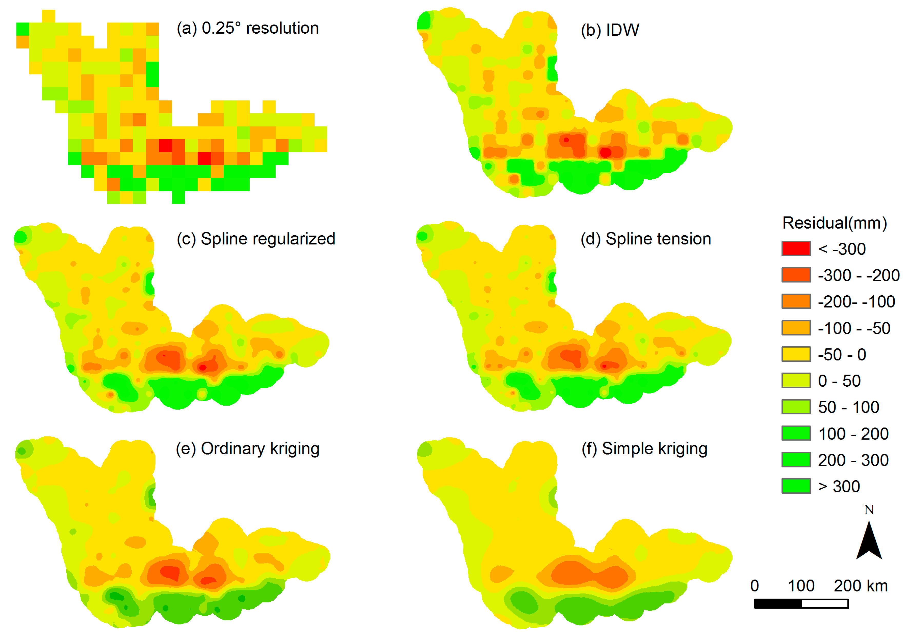
- In the process of downscaling satellite precipitation datasets with environmental variables, it was critical to select a suitable downscaling procedure to effectively conduct the downscaling based on the relationship between satellite precipitation and the NDVI, DEM. In this study, we established a hybrid downscaling method using a regression model with residual correction. According to the comparison of different regression models and residual interpolation methods, the GWRK method was accepted to conduct the downscaling of TRMM data. This indicated the non-stationary nature of the precipitation–NDVI and precipitation–DEM relationships and the spatial correlation structure of regression residuals needs to be considered when downscaling satellite precipitation datasets.
- Calibration with rain gauge data is an essential step for the downscaling-calibration procedure. Both the GDA and GRA calibration provided better annual precipitation when validated based on rain gauge data. The GRA outperformed the GDA method in terms of the validation metrics calculated.
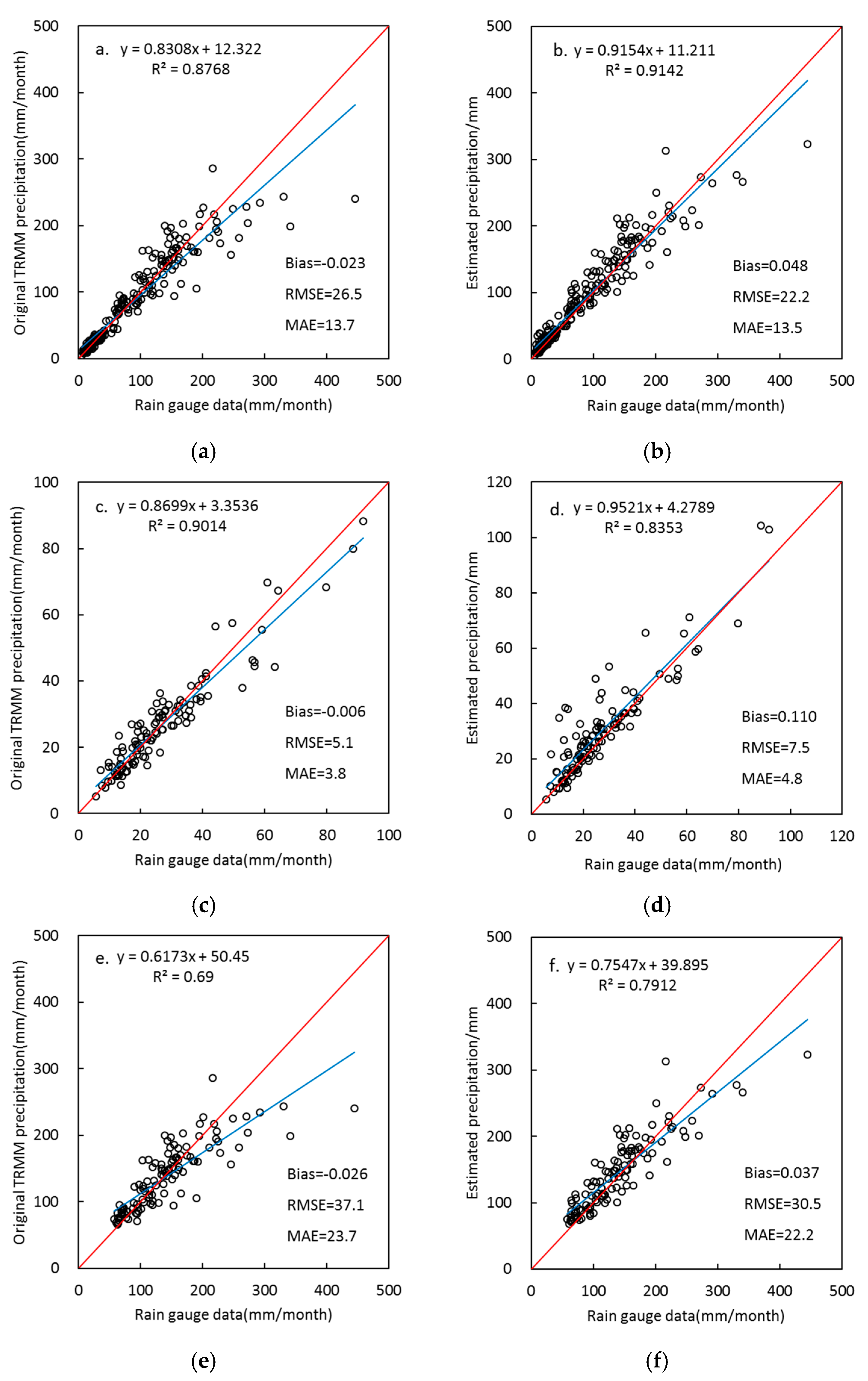
- Downscaled TRMM precipitation using environmental factors better described the spatial patterns of precipitation with more details at the spatial resolution of 1-km when compared with the original TRMM precipitation. Moreover, the simple disaggregation procedure based on the monthly fractions was practically used to disaggregate annual precipitation to monthly precipitation. The disaggregated 1-km monthly precipitation not only improved the spatial resolution, but also agreed well with rain gauge data (i.e., R2 = 0.72, RMSE = 161.0 mm, MAE = 127.5 mm, and Bias = 0.050 for annual downscaled precipitation during 2001–2015; R2 = 0.91, RMSE = 22.2 mm, MAE = 13.5 mm, and Bias = 0.048 for monthly downscaled precipitation during 2001–2015).
Acknowledgments
Author Contributions
Conflicts of Interest
Abbreviations
| TRMM | Tropical Rainfall Measuring Mission |
| NDVI | Normalized Difference Vegetation Index |
| GWR | Geographically-weighted regression |
| MLR | Multiple linear regression |
| ANN | Artificial neural network |
| GDA | Geographical difference analysis |
| GRA | Geographical ratio analysis |
| HSPD | High-spatial-resolution precipitation data |
| IDW | Inverse distance weighted |
| PRISM | Parameter-elevation Regressions on Independent Slopes Model |
| OPM | Orographic Precipitation Model |
| ASOADeK | Auto-Searched Orographic and Atmospheric Effects Detrended Kriging |
| GPCP | The Global Precipitation Climatology Project |
| GSMaP | The Global Satellite Mapping of Precipitation |
| CHIRPS | The Climate Hazards Group InfraRed Precipitation with Station data |
| MSWEP | The Multi-Source Weighted-Ensemble Precipitation |
| PERSIANN-CDR | The Precipitation Estimation from Remotely Sensed Information using Artificial Neural Networks-Climate Data Record |
| GPM | The Global Precipitation Measurement |
| NEXRAD | Next-Generation Radar |
| DEM | Digital elevation model |
| RGS | Rain gauge stations |
| NASA | National Aeronautics and Space Administration |
| JAXA | Japan Aerospace Exploration Agency |
| MODIS | Terra Moderate Resolution Imaging Spectroradiometer |
| IGBP | The International Geosphere Biosphere Program |
| SRTM | Shuttle Radar Topographic Mission |
| MLP | Multi-layer perceptron |
| R2 | The coefficient of determination |
| RMSE | The root mean square error |
| MAE | The mean absolute error |
| LOOCV | Leave-one-out Cross Validation |
| RK | Regression Kriging |
| GWRK | Geographically Weighted Regression Kriging |
| GPCC | The Global Precipitation Climatology Centre |
| IMERG | The Integrated Multi-satellitE Retrievals for GPM |
References
- Hu, Q.; Yang, D.; Wang, Y.; Yang, H. Accuracy and spatio-temporal variation of high resolution satellite rainfall estimate over the Ganjiang River Basin. Sci. China Technol. Sci. 2013, 56, 853–865. [Google Scholar] [CrossRef]
- Jia, S.; Zhu, W.; Lű, A.; Yan, T. A statistical spatial downscaling algorithm of TRMM precipitation based on NDVI and DEM in the Qaidam Basin of China. Remote Sens. Environ. 2011, 115, 3069–3079. [Google Scholar] [CrossRef]
- Li, M.; Shao, Q. An improved statistical approach to merge satellite rainfall estimates and raingauge data. J. Hydrol. 2010, 385, 51–64. [Google Scholar] [CrossRef]
- Goodrich, D.; Faurès, J.; Woolhiser, D.; Lane, L.; Sorooshian, S. Measurement and analysis of small-scale convective storm rainfall variability. J. Hydrol. 1995, 173, 283–308. [Google Scholar] [CrossRef]
- Goovaerts, P. Geostatistical approaches for incorporating elevation into the spatial interpolation of rainfall. J. Hydrol. 2000, 228, 113–129. [Google Scholar] [CrossRef]
- Guo, H.; Bao, A.; Liu, T.; Ndayisaba, F.; He, D.; Kurban, A.; Maeyer, P.D. Meteorological drought analysis in the Lower Mekong Basin using satellite-based long-term CHIRPS product. Sustainability 2017, 9, 901. [Google Scholar] [CrossRef]
- Simons, G.; Bastiaanssen, W.; Ngô, L.; Hain, C.; Anderson, M.; Senay, G. Integrating global satellite-derived data products as a pre-analysis for hydrological modelling studies: A case study for the Red River Basin. Remote Sens. 2016, 8, 279. [Google Scholar] [CrossRef]
- Grimes, D.I.F.; Diop, M. Satellite-based rainfall estimation for river flow forecasting in Africa. I: Rainfall estimates and hydrological forecasts. Hydrol. Sci. J. 2003, 48, 567–584. [Google Scholar] [CrossRef]
- Wheater, H.S.; Isham, V.S.; Cox, D.R.; Chandler, R.E. Spatial-temporal rainfall fields: Modelling and statistical aspects. Hydrol. Earth Syst. Sci. 2000, 4, 581–601. [Google Scholar] [CrossRef]
- Xie, P.; Arkin, P.A. Analyses of global monthly precipitation using gauge observations, satellite estimates, and numerical model predictions. J. Clim. 1996, 9, 840–858. [Google Scholar] [CrossRef]
- Fang, J.; Du, J.; Xu, W.; Shi, P.; Li, M.; Ming, X. Spatial downscaling of TRMM precipitation data based on the orographical effect and meteorological conditions in a mountainous area. Adv. Water Resour. 2013, 61, 42–50. [Google Scholar] [CrossRef]
- Gao, Z.; Long, D.; Tang, G.; Zeng, C.; Huang, J.; Hong, Y. Assessing the potential of satellite-based precipitation estimates for flood frequency analysis in ungauged or poorly gauged tributaries of China’s Yangtze River basin. J. Hydrol. 2017, 550, 478–496. [Google Scholar] [CrossRef]
- Hutchinson, M.F. The application of thin plate smoothing splines to continent-wide data assimilation. Data Assim. Syst. 1991, 27, 104–113. [Google Scholar]
- Zhang, X.; Srinivasan, R. GIS-based spatial precipitation estimation: A comparison of geostatistical approaches. J. Am. Water Resour. Assoc. 2009, 45, 894–906. [Google Scholar] [CrossRef]
- Hans, W. Multivariate Geostatistics: An Introduction with Applications; Springer: Berlin, Germany, 2003. [Google Scholar]
- Daly, C.; Neilson, R.P.; Phillips, D.L. A statistical-topographic model for mapping climatological precipitation over mountain terrain. J. Appl. Meteorol. 1994, 33, 140–158. [Google Scholar] [CrossRef]
- Shamir, E.; Rimmer, A.; Georgakakos, K.P. The use of an orographic precipitation model to assess the precipitation spatial distribution in Lake Kinneret Watershed. Water 2016, 8, 591. [Google Scholar] [CrossRef]
- Guan, H.D.; Wilson, J.L.; Makhnin, O. Geostatistical mapping of mountain precipitation incorporating Autosearched Effects of Terrain and Climatic Characteristic. J. Hydrometeorol. 2005, 6, 1018–1031. [Google Scholar] [CrossRef]
- Hong, Y.; Nix, H.A.; Hutchinson, M.F.; Booth, T.H. Spatial interpolation of monthly mean climate data for China. Int. J. Climatol. 2005, 25, 1369–1379. [Google Scholar] [CrossRef]
- Mahesh, C.; Prakash, S.; Sathiyamoorthy, V.; Gairola, R.M. Artificial neural network based microwave precipitation estimation using scattering index and polarization corrected temperature. Atmos. Res. 2011, 102, 358–364. [Google Scholar] [CrossRef]
- Huffman, G.J.; Adler, R.F.; Arkin, P.; Chang, A.; Ferraro, R.; Gruber, A.; Janowiak, J.; Mcnab, A.; Rudolf, B.; Schneider, U. The Global Precipitation Climatology Project (GPCP) combined precipitation dataset. Bull. Am. Meteorol. Soc. 1997, 78, 5–20. [Google Scholar] [CrossRef]
- Kubota, T.; Shige, S.; Hashizume, H.; Aonashi, K.; Takahashi, N.; Seto, S.; Takayabu, Y.N.; Ushio, T.; Nakagawa, K.; Iwanami, K. Global precipitation map using satellite-borne microwave radiometers by the GSMaP project: Production and validation. IEEE Trans. Geosci. Remote Sens. 2007, 45, 2259–2275. [Google Scholar] [CrossRef]
- Funk, C.; Peterson, P.; Landsfeld, M.; Pedreros, D.; Verdin, J.; Shukla, S.; Husak, G.; Rowland, J.; Harrison, L.; Hoell, A. The climate hazards infrared precipitation with stations—A new environmental record for monitoring extremes. Sci. Data 2015, 2, 150066. [Google Scholar] [CrossRef] [PubMed]
- Beck, H.E.; van Dijk, A.I.J.M.; Levizzani, V.; Schellekens, J.; Miralles, D.G.; Martens, B.; de Roo, A. MSWEP: 3-hourly 0.25° global gridded precipitation (1979–2015) by merging gauge, satellite, and reanalysis data. Hydrol. Earth Syst. Sci. 2017, 21, 589–615. [Google Scholar] [CrossRef]
- Hsu, K.; Gao, X.; Sorooshian, S.; Gupta, H.V. Precipitation estimation from remotely sensed information using artificial neural networks. J. Appl. Meteorol. 1997, 36, 1176–1190. [Google Scholar] [CrossRef]
- Kummerow, C.; Barnes, W.; Kozu, T.; Shiue, J.; Simpson, J. The Tropical Rainfall Measuring Mission (TRMM) sensor package. J. Atmos. Ocean. Technol. 1998, 15, 809. [Google Scholar] [CrossRef]
- Huffman, G.J.; Adler, R.F.; Bolvin, D.T.; Gu, G.; Nelkin, E.J.; Bowman, K.P.; Hong, Y.; Stocker, E.F.; Wolff, D.B. The TRMM Multisatellite Precipitation Analysis (TMPA): Quasi-global, multiyear, combined-sensor precipitation estimates at fine scales. J. Hydrometeorol. 2007, 8, 38–55. [Google Scholar] [CrossRef]
- Hou, A.Y.; Kakar, R.K.; Neeck, S.; Azarbarzin, A.A.; Kummerow, C.D.; Kojima, M.; Oki, R.; Nakamura, K.; Iguchi, T. The Global precipitation measurement mission. Bull. Am. Meteorol. Soc. 2014, 95, 701–722. [Google Scholar] [CrossRef]
- Tian, Y.; Peters-Lidard, C.D.; Choudhury, B.J.; Garcia, M. Multitemporal analysis of TRMM-based satellite precipitation products for land data assimilation applications. J. Hydrometeorol. 2007, 8, 1165–1183. [Google Scholar] [CrossRef]
- Naumann, G.; Barbosa, P.; Carrao, H.; Singleton, A.; Vogt, J. Monitoring drought conditions and their uncertainties in Africa using TRMM data. J. Appl. Meteorol. Climatol. 2012, 51, 1867–1874. [Google Scholar] [CrossRef]
- Wei, W.; Hui, L.; Yang, D.; Khem, S.; Yang, J.; Gao, B.; Peng, X.; Pang, Z. Modelling hydrologic processes in the Mekong River Basin using a distributed model driven by satellite precipitation and rain gauge observations. PLoS ONE 2016, 11, e0152229. [Google Scholar]
- Immerzeel, W.W.; Rutten, M.M.; Droogers, P. Spatial downscaling of TRMM precipitation using vegetative response on the Iberian Peninsula. Remote Sens. Environ. 2009, 113, 362–370. [Google Scholar] [CrossRef]
- Wang, J.; Georgakakos, K.P. Validation and sensitivities of dynamic precipitation simulation for winter events over the Folsom Lake Watershed: 1964–1999. Mon. Weather Rev. 2003, 133, 3–19. [Google Scholar] [CrossRef]
- Meersmans, J.; Van Weverberg, K.; De Baets, S.; De Ridder, F.; Palmer, S.J.; van Wesemael, B.; Quine, T.A. Mapping mean total annual precipitation in Belgium, by investigating the scale of topographic control at the regional scale. J. Hydrol. 2016, 540, 96–105. [Google Scholar] [CrossRef]
- Sokol, Z.; Bližňák, V. Areal distribution and precipitation–altitude relationship of heavy short-term precipitation in the Czech Republic in the warm part of the year. Atmos. Res. 2009, 94, 652–662. [Google Scholar] [CrossRef]
- Jing, W.; Yang, Y.; Yue, X.; Zhao, X. A comparison of different regression algorithms for downscaling monthly satellite-based precipitation over North China. Remote Sens. 2016, 8, 835. [Google Scholar] [CrossRef]
- Reid, I. The influence of slope aspect on precipitation receipt. Weather 1973, 28, 490–494. [Google Scholar] [CrossRef]
- Smith, R.B. The influence of mountains on the atmosphere. Adv. Geophys. 1979, 21, 87–230. [Google Scholar]
- Badas, M.G.; Deidda, R.; Piga, E. Orographic influences in rainfall downscaling. Adv. Geosci. 2005, 2, 285–292. [Google Scholar] [CrossRef]
- Guan, H.D.; Wilson, J.L.; Xie, H.J. A cluster-optimizing regression-based approach for precipitation spatial downscaling in mountainous terrain. J. Hydrol. 2009, 375, 578–588. [Google Scholar] [CrossRef]
- Duan, Z.; Bastiaanssen, W.G.M. First results from Version 7 TRMM 3B43 precipitation product in combination with a new downscaling–calibration procedure. Remote Sens. Environ. 2013, 131, 1–13. [Google Scholar] [CrossRef]
- Jing, W.; Yang, Y.; Yue, X.; Zhao, X. A spatial downscaling algorithm for satellite-based precipitation over the Tibetan Plateau based on NDVI, DEM, and land surface temperature. Remote Sens. 2016, 8, 655. [Google Scholar] [CrossRef]
- Duffaut Espinosa, L.A.; Posadas, A.N.; Carbajal, M.; Quiroz, R. Multifractal downscaling of rainfall using normalized difference vegetation index (NDVI) in the Andes Plateau. PLoS ONE 2017, 12, e0168982. [Google Scholar] [CrossRef] [PubMed]
- Immerzeel, W.W.; Quiroz, R.A.; De Jong, S.M. Understanding precipitation patterns and land use interaction in Tibet using harmonic analysis of SPOT VGT-S10 NDVI time series. Int. J. Remote Sens. 2005, 26, 2281–2296. [Google Scholar] [CrossRef]
- Quiroz, R.; Yarlequé, C.; Posadas, A.; Mares, V.; Immerzeel, W.W. Improving daily rainfall estimation from NDVI using a wavelet transform. Environ. Model. Softw. 2011, 26, 201–209. [Google Scholar] [CrossRef]
- Hunink, J.E.; Immerzeel, W.W.; Droogers, P. A high-resolution precipitation 2-step mapping procedure (HiP2P): Development and application to a tropical mountainous area. Remote Sens. Environ. 2014, 140, 179–188. [Google Scholar] [CrossRef]
- Alexakis, D.D.; Tsanis, I.K. Comparison of multiple linear regression and artificial neural network models for downscaling TRMM precipitation products using MODIS data. Environ. Earth Sci. 2016, 75, 1077. [Google Scholar] [CrossRef]
- Chen, F.; Liu, Y.; Liu, Q.; Li, X. Spatial downscaling of TRMM 3B43 precipitation considering spatial heterogeneity. Int. J. Remote Sens. 2014, 35, 3074–3093. [Google Scholar] [CrossRef]
- Xu, S.; Wu, C.; Wang, L.; Gonsamo, A.; Shen, Y.; Niu, Z. A new satellite-based monthly precipitation downscaling algorithm with non-stationary relationship between precipitation and land surface characteristics. Remote Sens. Environ. 2015, 162, 119–140. [Google Scholar] [CrossRef]
- Condom, T.; Rau, P.; Espinoza, J.C. Correction of TRMM 3B43 monthly precipitation data over the mountainous areas of Peru during the period 1998–2007. Hydrol. Process. 2011, 25, 1924–1933. [Google Scholar] [CrossRef]
- Franchito, S.H.; Rao, V.B.; Vasques, A.C.; Santo, C.M.E.; Conforte, J.C. Validation of TRMM precipitation radar monthly rainfall estimates over Brazil. J. Geophys. Res. Atmos. 2009, 114, 356–360. [Google Scholar] [CrossRef]
- Almazroui, M. Calibration of TRMM rainfall climatology over Saudi Arabia during 1998–2009. Atmos. Res. 2011, 99, 400–414. [Google Scholar] [CrossRef]
- Cheema, M.J.M.; Bastiaanssen, W.G.M. Local calibration of remotely sensed rainfall from the TRMM satellite for different periods and spatial scales in the Indus Basin. Int. J. Remote Sens. 2012, 33, 2603–2627. [Google Scholar] [CrossRef]
- Li, Y.G.; He, D.M.; Ye, C.Q. Spatial and temporal variation of runoff of Red River Basin in Yunnan. J. Geogr. Sci. 2008, 18, 308–318. [Google Scholar] [CrossRef]
- Li, Y.G.; He, D.M. The spatial and temporal variation of NDVI and its relationships to the climatic factors in Red River Basin. J. Mt. Sci. 2009, 27, 333–340. (In Chinese) [Google Scholar]
- Zhou, X.; Ni, G.H.; Shen, C.; Sun, T. Remapping annual precipitation in mountainous areas based on vegetation patterns: A case study in the Nu River basin. Hydrol. Earth Syst. Sci. 2017, 21, 999–1015. [Google Scholar] [CrossRef]
- Caúla, R.H.; Oliveira-Júnior, J.F.; Gois, G.; Delgado, R.C.; Pimentel, L.C.G.; Teodoro, P.E. Nonparametric statistics applied to fire foci obtained by meteorological satellites and their relationship to the MCD12Q1 product in the state of Rio de Janeiro, Southeast-Brazil. Land Degrad. Dev. 2017, 28, 1056–1067. [Google Scholar] [CrossRef]
- Rodríguez, E.; Morris, C.S.; Belz, J.E. A global assessment of the SRTM performance. Photogramm. Eng. Remote Sens. 2006, 72, 249–260. [Google Scholar] [CrossRef]
- Teng, H.; Shi, Z.; Ma, Z.; Li, Y. Estimating spatially downscaled rainfall by regression kriging using TRMM precipitation and elevation in Zhejiang Province, southeast China. Int. J. Remote Sens. 2014, 35, 7775–7794. [Google Scholar] [CrossRef]
- Park, N.-W. Spatial downscaling of TRMM precipitation using geostatistics and fine scale environmental variables. Adv. Meteorol. 2013, 2013, 1–9. [Google Scholar] [CrossRef]
- Naoum, S.; Tsanis, I.K. Temporal and spatial variation of annual rainfall on the island of Crete, Greece. Hydrol. Process. 2003, 17, 1899–1922. [Google Scholar] [CrossRef]
- Lees, B.G. Neural network applications in the geosciences: An introduction. Comput. Geosci. 1996, 22, 955–957. [Google Scholar] [CrossRef]
- Tomassetti, B.; Verdecchia, M.; Giorgi, F. NN5: A neural network based approach for the downscaling of precipitation fields—Model description and preliminary results. J. Hydrol. 2009, 367, 14–26. [Google Scholar] [CrossRef]
- Kumar, R.; Gairola, R.M.; Sarkar, A.; Agarwal, V.K. Rainfall retrieval from TRMM radiometric channels using artificial neural networks. Indian J. Radio Space Phys. 2007, 36, 114–127. [Google Scholar]
- Nielsen, R.H. Counterpropagation networks. Appl. Opt. 1987, 26, 4979–4984. [Google Scholar] [CrossRef] [PubMed]
- The MathWorks, Inc. MATLAB and Neural Network Toolbox Release R2012a; The MathWorks, Inc.: Natick, MA, USA, 2012. [Google Scholar]
- Foody, G.M. Geographical weighting as a further refinement to regression modelling: An example focused on the NDVI–Rainfall relationship. Remote Sens. Environ. 2003, 88, 283–293. [Google Scholar] [CrossRef]
- Fotheringham, A.S.; Brunsdon, C.; Charlton, M. Geographically Weighted Regression: The Analysis of Spatially Varying Relationships; Wiley: New York, NY, USA, 2002. [Google Scholar]
- Gao, Y.; Huang, J.; Li, S.; Li, S. Spatial pattern of non-stationarity and scale-dependent relationships between NDVI and climatic factors—A case study in Qinghai-Tibet Plateau, China. Ecol. Indic. 2012, 20, 170–176. [Google Scholar] [CrossRef]
- Lloyd, C.D. Assessing the effect of integrating elevation data into the estimation of monthly precipitation in Great Britain. J. Hydrol. 2005, 308, 128–150. [Google Scholar] [CrossRef]
- Sieck, L.C.; Burges, S.J.; Steiner, M. Challenges in obtaining reliable measurements of point rainfall. Water Resour. Res. 2007, 43. [Google Scholar] [CrossRef]
- Maggioni, V.; Meyers, P.C.; Robinson, M.D. A review of merged high-resolution satellite precipitation product accuracy during the Tropical Rainfall Measuring Mission (TRMM) era. J. Hydrom. 2016, 17, 1101–1117. [Google Scholar] [CrossRef]
- Prakash, S.; Mitra, A.K.; AghaKouchak, A.; Pai, D.S. Error characterization of TRMM Multisatellite Precipitation Analysis (TMPA-3B42) products over India for different seasons. J. Hydrol. 2015, 529, 1302–1312. [Google Scholar] [CrossRef]
- Zhang, Q.; Shi, P.; Singh, V.P.; Fan, K.; Huang, J. Spatial downscaling of TRMM-based precipitation data using vegetative response in Xinjiang, China. Int. J. Climatol. 2016, 37, 3895–3909. [Google Scholar] [CrossRef]
- Shi, Y.; Song, L. Spatial downscaling of monthly TRMM precipitation based on EVI and other geospatial variables over the Tibetan Plateau from 2001 to 2012. Mt. Res. Dev. 2015, 35, 180–194. [Google Scholar] [CrossRef]
- Wang, J.; Price, K.P.; Rich, P.M. Spatial patterns of NDVI in response to precipitation and temperature in the central Great Plains. Int. J. Remote Sens. 2001, 22, 3827–3844. [Google Scholar] [CrossRef]
- Barbosa, H.A.; Kumar, T.V.L. Influence of rainfall variability on the vegetation dynamics over Northeastern Brazil. J. Arid Environ. 2016, 124, 377–387. [Google Scholar] [CrossRef]
- Shi, Y.; Song, L.; Xia, Z.; Lin, Y.; Myneni, R.; Choi, S.; Wang, L.; Ni, X.; Lao, C.; Yang, F. Mapping annual precipitation across Mainland China in the period 2001–2010 from TRMM 3B43 product using spatial downscaling approach. Remote Sens. 2015, 7, 5849–5878. [Google Scholar] [CrossRef]
- Wang, H.; Chen, A.; Wang, Q.; He, B. Drought dynamics and impacts on vegetation in China from 1982 to 2011. Ecol. Eng. 2015, 75, 303–307. [Google Scholar] [CrossRef]
- Prudhomme, C.; Reed, D.W. Mapping extreme rainfall in a mountainous region using geostatistical techniques: A case study in Scotland. Int. J. Climatol. 1999, 19, 1337–1356. [Google Scholar] [CrossRef]
- Daly, C. Guidelines for assessing the suitability of spatial climate data sets. Int. J. Climatol. 2006, 26, 707–721. [Google Scholar] [CrossRef]
- Moral, F.J. Comparison of different geostatistical approaches to map climate variables: Application to precipitation. Int. J. Climatol. 2010, 30, 620–631. [Google Scholar] [CrossRef]
- Bostan, P.A.; Heuvelink, G.B.M.; Akyurek, S.Z. Comparison of regression and kriging techniques for mapping the average annual precipitation of Turkey. Int. J. Appl. Earth Obs. Geoinf. 2012, 19, 115–126. [Google Scholar] [CrossRef]
- Li, J.; Heap, A.D. Spatial interpolation methods applied in the environmental sciences: A review. Environ. Model. Softw. 2014, 53, 173–189. [Google Scholar] [CrossRef]
- Pereira, P.; Oliva, M.; Misiune, I. Spatial interpolation of precipitation indexes in Sierra Nevada (Spain): Comparing the performance of some interpolation methods. Theor. Appl. Climatol. 2015, 126, 683–698. [Google Scholar] [CrossRef]
- Wagner, P.D.; Fiener, P.; Wilken, F.; Kumar, S.; Schneider, K. Comparison and evaluation of spatial interpolation schemes for daily rainfall in data scarce regions. J. Hydrol. 2012, 464–465, 388–400. [Google Scholar] [CrossRef]
- Hengl, T.; Heuvelink, G.B.M.; Rossiter, D.G. About regression-kriging: From equations to case studies. Comput. Geosci. 2007, 33, 1301–1315. [Google Scholar] [CrossRef]
- Kumar, S.; Lal, R.; Liu, D. A geographically weighted regression kriging approach for mapping soil organic carbon stock. Geoderma 2012, 189–190, 627–634. [Google Scholar] [CrossRef]
- Harris, P.; Fotheringham, A.S.; Crespo, R.; Charlton, M. The use of geographically weighted regression for spatial prediction: An evaluation of models using simulated data sets. Math. Geosci. 2010, 42, 657–680. [Google Scholar] [CrossRef]
- Imran, M.; Stein, A.; Zurita-Milla, R. Using geographically weighted regression kriging for crop yield mapping in West Africa. Int. J. Geogr. Inf. Sci. 2015, 29, 234–257. [Google Scholar] [CrossRef]
- Zhao, H.; Yang, B.; Yang, S.; Huang, Y.; Dong, G.; Bai, J.; Wang, Z. Systematical estimation of GPM-based global satellite mapping of precipitation products over China. Atmos. Res. 2018, 201, 206–217. [Google Scholar] [CrossRef]
- Prakash, S.; Mitra, A.K.; AghaKouchak, A.; Liu, Z.; Norouzi, H.; Pai, D.S. A preliminary assessment of GPM-based multi-satellite precipitation estimates over a monsoon dominated region. J. Hydrol. 2016, 56, 853–865. [Google Scholar] [CrossRef]


| Year | 2001 (Wet) | 2005 (Normal) | 2009 (Dry) | 2001–2015 (Averaged) | |
|---|---|---|---|---|---|
| MLR | R2 | 0.44 (0.32, 0.55) | 0.52 (0.42, 0.61) | 0.58 (0.50, 0.66) | 0.59 (0.49, 0.67) |
| RMSE | 241 (216, 265) | 241 (214, 268) | 231 (207, 255) | 221 (197, 244) | |
| MAE | 194 (173, 215) | 185 (163, 207) | 184 (165, 205) | 172 (152, 192) | |
| Bias | 0.010 (−0.014, 0.038) | 0.014 (−0.019, 0.047) | 0.017 (−0.022, 0.052) | 0.014 (−0.015, 0.043) | |
| ANN | R2 | 0.90 (0.86, 0.93) | 0.90 (0.85, 0.93) | 0.92 (0.90, 0.95) | 0.91 (0.86, 0.95) |
| RMSE | 112 (97, 126) | 115 (99, 134) | 101 (88, 114) | 105 (85, 124) | |
| MAE | 85 (73, 96) | 88 (78, 100) | 75 (65, 85) | 73 (62, 84) | |
| Bias | 0.030 (0.019, 0.042) | 0.001 (−0.015, 0.016) | 0.025 (0.009, 0.041) | −0.016 (−0.029, −0.004) | |
| GWR | R2 | 0.87 (0.82, 0.91) | 0.89 (0.85, 0.92) | 0.90 (0.86, 0.93) | 0.90 (0.86, 0.93) |
| RMSE | 117 (99, 137) | 119 (103, 137) | 114 (97, 131) | 110 (92, 127) | |
| MAE | 78 (66, 91) | 82 (71, 96) | 76 (65, 88) | 73 (61, 86) | |
| Bias | −0.000 (−0.012, 0.012) | 0.000 (−0.015, 0.016) | 0.000 (−0.017, 0.016) | 0.002 (−0.012, 0.016) | |
| Interpolation Methods | IDW | Spline Regularized | Spline Tension | Ordinary Kriging | Simple Kriging |
|---|---|---|---|---|---|
| RMSE | 97.56 (83.11, 114.26) | 96.50 (82.10, 113.86) | 96.39 (81.95, 113.00) | 96.47 (82.05, 113.28) | 95.56 (81.23, 112.40) |
| MAE | 67.89 (57.68, 78.92) | 67.73 (57.83, 78.62) | 67.48 (57.35, 78.41) | 67.45 (57.32, 78.39) | 66.86 (56.95, 77.77) |
| Year | Datasets | Mean (mm) | R2 | RMSE (mm) | MAE (mm) | Bias |
|---|---|---|---|---|---|---|
| 2001 (Wet) | RGS | 1276 | ||||
| V7 | 1210 | 0.36 (0.12, 0.65) | 246 (107, 399) | 159 (82, 267) | −0.050 (−0.133, 0.027) | |
| DS | 1218 | 0.35 (0.06, 0.66) | 245 (125, 354) | 171 (98, 260) | −0.044 (−0.125, 0.033) | |
| DSGDA | 1290 | 0.54 (0.21, 0.80) | 198 (125, 266) | 155 (102, 217) | 0.012 (−0.055, 0.078) | |
| DSGRA | 1279 | 0.55 (0.22, 0.80) | 196 (123, 264) | 155 (101, 215) | 0.004 (−0.064, 0.070) | |
| 2005 (Normal) | RGS | 1035 | ||||
| V7 | 951 | 0.57 (0.18, 0.87) | 243 (105, 411) | 156 (82, 263) | −0.078 (−0.174, 0.015) | |
| DS | 974 | 0.60 (0.06, 0.90) | 211 (127, 313) | 159 (100, 230) | −0.056 (−0.136, 0.031) | |
| DSGDA | 1053 | 0.66 (0.12, 0.92) | 190 (116, 271) | 142 (88, 203) | 0.020 (−0.060, 0.109) | |
| DSGRA | 1068 | 0.65 (0.14, 0.92) | 185 (115, 254) | 137 (84, 198) | 0.035 (−0.045, 0.121) | |
| 2009 (Dry) | RGS | 826 | ||||
| V7 | 791 | 0.45 (0.12, 0.76) | 235 (153, 333) | 184 (123, 255) | −0.034 (−0.149, 0.097) | |
| DS | 810 | 0.56 (0.08, 0.87) | 200 (159, 239) | 169 (120, 215) | −0.015 (−0.112, 0.105) | |
| DSGDA | 831 | 0.62 (0.11, 0.89) | 181 (142, 222) | 157 (117, 197) | 0.010 (−0.088, 0.118) | |
| DSGRA | 828 | 0.63 (0.12, 0.90) | 175 (134, 217) | 151 (111, 191) | 0.006 (−0.087, 0.110) | |
| 2001–2015 (Averaged) | RGS | 1011 | ||||
| V7 | 988 | 0.64 (0.37, 0.84) | 202 (111, 316) | 142 (85, 220) | −0.021 (−0.109, 0.073) | |
| DS | 1005 | 0.63 (0.17, 0.89) | 187 (123, 254) | 144 (91, 201) | −0.005 (−0.081, 0.083) | |
| DSGDA | 1066 | 0.71 (0.26, 0.93) | 170 (124, 211) | 137 (92, 186) | 0.055 (−0.018, 0.139) | |
| DSGRA | 1061 | 0.72 (0.27, 0.93) | 161 (115, 201) | 128 (83, 172) | 0.050 (−0.017, 0.130) |
© 2018 by the authors. Licensee MDPI, Basel, Switzerland. This article is an open access article distributed under the terms and conditions of the Creative Commons Attribution (CC BY) license (http://creativecommons.org/licenses/by/4.0/).
Share and Cite
Zhang, Y.; Li, Y.; Ji, X.; Luo, X.; Li, X. Fine-Resolution Precipitation Mapping in a Mountainous Watershed: Geostatistical Downscaling of TRMM Products Based on Environmental Variables. Remote Sens. 2018, 10, 119. https://doi.org/10.3390/rs10010119
Zhang Y, Li Y, Ji X, Luo X, Li X. Fine-Resolution Precipitation Mapping in a Mountainous Watershed: Geostatistical Downscaling of TRMM Products Based on Environmental Variables. Remote Sensing. 2018; 10(1):119. https://doi.org/10.3390/rs10010119
Chicago/Turabian StyleZhang, Yueyuan, Yungang Li, Xuan Ji, Xian Luo, and Xue Li. 2018. "Fine-Resolution Precipitation Mapping in a Mountainous Watershed: Geostatistical Downscaling of TRMM Products Based on Environmental Variables" Remote Sensing 10, no. 1: 119. https://doi.org/10.3390/rs10010119