Comparison of Different Machine Learning Approaches for Monthly Satellite-Based Soil Moisture Downscaling over Northeast China


1
State Key Laboratory of Resources and Environmental Information System, Institute of Geographic Sciences and Natural Resources Research, Chinese Academy of Sciences, Beijing 100101, China
2
University of Chinese Academy of Sciences, Beijing 100049, China
3
Jiangsu Center for Collaborative Innovation in Geographical Information Resource Development and Application, Nanjing 210023, China
4
Guangzhou Institute of Geography, Guangzhou 510070, China
5
Key Laboratory of Guangdong for Utilization of Remote Sensing and Geographical Information System, Guangzhou 510070, China
6
Guangdong Open Laboratory of Geospatial Information Technology and Application, Guangzhou 510070, China
*
Author to whom correspondence should be addressed.
Remote Sens. 2018, 10(1), 31; https://doi.org/10.3390/rs10010031
Submission received: 16 November 2017
/
Revised: 20 December 2017
/
Accepted: 22 December 2017
/
Published: 25 December 2017
(This article belongs to the Special Issue Retrieval, Validation and Application of Satellite Soil Moisture Data)
Abstract
:Although numerous satellite-based soil moisture (SM) products can provide spatiotemporally continuous worldwide datasets, they can hardly be employed in characterizing fine-grained regional land surface processes, owing to their coarse spatial resolution. In this study, we proposed a machine-learning-based method to enhance SM spatial accuracy and improve the availability of SM data. Four machine learning algorithms, including classification and regression trees (CART), K-nearest neighbors (KNN), Bayesian (BAYE), and random forests (RF), were implemented to downscale the monthly European Space Agency Climate Change Initiative (ESA CCI) SM product from 25-km to 1-km spatial resolution. During the regression, the land surface temperature (including daytime temperature, nighttime temperature, and diurnal fluctuation temperature), normalized difference vegetation index, surface reflections (red band, blue band, NIR band and MIR band), and digital elevation model were taken as explanatory variables to produce fine spatial resolution SM. We chose Northeast China as the study area and acquired corresponding SM data from 2003 to 2012 in unfrozen seasons. The reconstructed SM datasets were validated against in-situ measurements. The results showed that the RF-downscaled results had superior matching performance to both ESA CCI SM and in-situ measurements, and can positively respond to precipitation variation. Additionally, the RF was less affected by parameters, which revealed its robustness. Both CART and KNN ranked second. Compared to KNN, CART had a relatively close correlation with the validation data, but KNN showed preferable precision. Moreover, BAYE ranked last with significantly abnormal regression values.
1. Introduction
Soil moisture (SM) is a key indicator for characterizing agricultural drought, hydrological processes, land surface evapotranspiration, and regional climate change [1,2,3,4]. A systematic analysis of SM is conducive to acquiring accurate crop growth information as well as yield prediction [5,6,7]. The SM observations provided by ground-based networks (e.g., the International Soil Moisture Network [8], the Global Soil Moisture Data Bank [9], the U.S. SCAN network [10] and Chinese Ecosystem Research Field Observational Stations Network [11]) have been effective sources of long time series of regional soil water data [12,13,14]. However, considering that there are a limited number of ground stations with uneven distribution in an observation network, it is hard to reflect the SM of an entire region on the same scale [15,16,17,18]. For example, the stations could be densely distributed over flat terrain and key research areas, with a thin distribution over uncultivated mountainous environments with high altitude, steep slopes and dangerous terrain. In addition, because every single station only represents the SM of a restricted homogeneous region and all the in-situ measurements could hardly cover the entire required time span, it is less suitable to use ground station data for broad and long-term analysis [12,13,14]. After nearly two decades of development of aerospace technology, attention has increasingly been paid to satellite-based SM, as it can provide spatiotemporally continuous datasets on a large scale [19,20]. Currently, there are various types of satellites that provide near real-time SM products, such as the passive (radiometer) microwave-based Advanced Microwave Scanning Radiometer-Earth Observing System (AMSR-E) [21], Advanced Microwave Scanning Radiometer 2 (AMSR2) [22], Soil Moisture Ocean Salinity (SMOS) [23], WindSat [24], active (radar) microwave-based Advanced Land Observation Satellite-Phased Array type L-band Synthetic Aperture Radar (ALOS PALSAR) [25], European Remote Sensing Satellites (ERS) [26], Sentinel-1 [27], a combination of active and passive microwave-based Soil Moisture Active Passive (SMAP) [28] and European Space Agency Climate Change Initiative (ESA CCI) [29]. In addition, physically based COsmic-ray Soil Moisture Interaction Code (COSMIC) is also an efficient method to acquire SM by data assimilation. Moreover, it can eliminate the bias between satellite-measured date and in-situ observation data [30].These SM datasets have been extensively made use of by many scholars. However, the coarse spatial resolution fails to meet the needs of studies for SM variations of specific regions [31].
To enhance the spatial resolution of the satellite-based SM products, a considerable body of research has been carried out to develop SM downscaling techniques. Some remarkable results have been achieved during the process of exploring different fine-resolution datasets. Mallick et al. [32] proposed a method that took advantage of the correlation between soil wetness and vegetation-modulated land surface temperature to derive an SM index [33]. Against this background, Fang et al. [34] constructed a pixel-based linear regression model to downscale passive microwave-based daily AMSR-E SM datasets by utilizing the triangular relationship between SM, vegetation cover and surface temperature. María Piles et al. [35] downscaled the SMOS-derived SM using a universal triangle algorithm with the Moderate Resolution Imaging Spectroradiometer (MODIS) [36] visible and infrared data, but the downscaled SM maps shows a high bias until the SMOS brightness temperature was added as a parameter. Srivastava et al. [37] compared four machine learning algorithms for downscaling SMOS SM data using the MODIS Terra level 3 Land Surface Temperature (LST) product with the superior performance of an artificial neural network (ANN). However, they did not take the decision tree-based algorithm into consideration, which is a mature supervised learning method. Peng et al. [38] constructed a simple nonlinear formula taking the vegetation temperature condition index as the only input parameter to get higher spatial resolution ESA CCI SM over the Yunnan province of China without considering terrain effects.
There exists a complicated nonlinear spatiotemporally changing relationship between SM and the LST, vegetation cover, and altitude [33,37,38,39,40,41,42,43]. Hence, it is, to some extent, inappropriate to implement a simple regression approach to downscale low-resolution heterogeneous SM datasets. Moreover, several machine learning regression algorithms have been broadly utilized in downscaling SM-relative subjects of remote sensing data, such as precipitation [39] and evapotranspiration [38]. Additionally, there is a great deal of research focusing on downscaling passive microwave satellite SM [34,35,37,41,42]. However, there is still a lack of studies focused on comparing diverse downscaling algorithms, especially by evaluating various machine learning downscaling methods over a combination of active and passive microwave-based SM products. K-nearest neighbors (KNN) is a mature regression method and simple machine learning algorithm [44]. In Bayesian regression (BAYE), a weighted integral rather than point estimation is employed to obtain posterior distributions [45]. In addition to these, classification and regression trees (CART) is an easily understood and commonly used supervised learning method [46]. By contrast, being an advanced algorithm containing multiple decision trees, the random forest (RF) often yields results with higher accuracy [47]. Consequently, we tested and compared four types of machine learning methods, including CART, KNN, BAYE and RF, to downscale ESA CCI SM over Northeast China to find a better algorithm for retrieving finer-resolution data in this study.
Moreover, because LST is closely associated to SM, which means its day–night would remarkably influence soil wetness [37,38,39], MODIS LST was involved in the downscaling process. Additionally, vegetation conditions such as coverage, growing stages, species composition, and root morphology could have complex and profound effects on soil water circulation [33,38,40,48]. Furthermore, with the increase in altitude, soil water tends to drain away more easily [43]. Thus, we applied the normalized difference vegetation index (NDVI), NDVI-related red band and near infrared band (NIR), blue band that promotes chlorophyll synthesis, mid infrared band (MIR) that reflects the intense absorption of soil water, and digital elevation model (DEM) as input parameters to downscale the monthly ESA CCI SM over Northeast China from 2003 to 2012 for the unfrozen months from April to October. The water area was removed before downscaling by a water mask extraction.
2. Study Area and Data Resources
2.1. Study Area
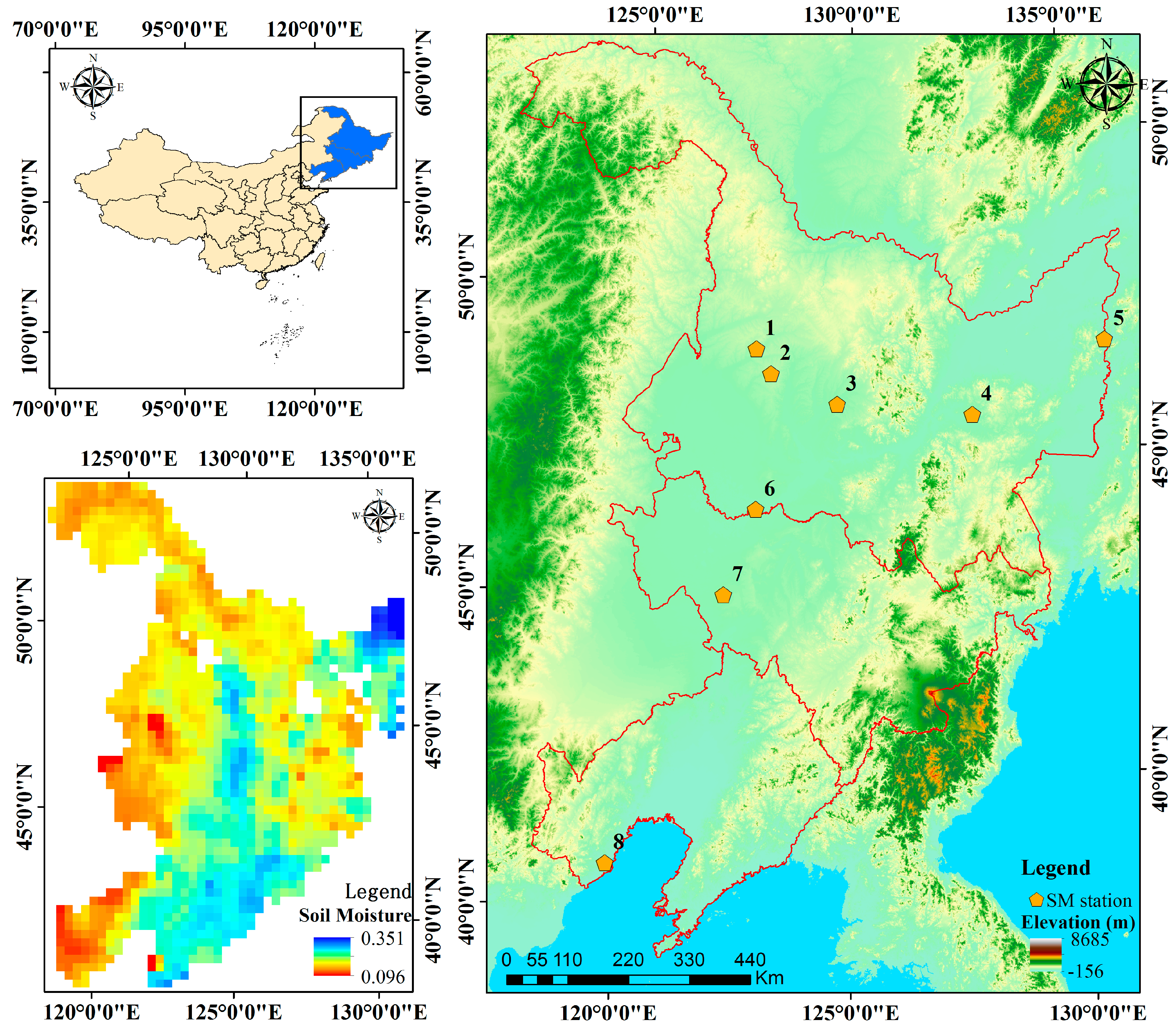
The three provinces of Northeast China, namely Heilongjiang, Jilin, and Liaoning Provinces, were chosen for this case study. They span approximately 787,300 km2 within 38.72°N–53.59°N and 121.00°E–135.19°E (Figure 1). The terrain in Northeast China is mainly dominated by plains and mountainous areas. Owing to the high latitude, this region generally belongs to the cold and mid-temperate monsoon climate with cold, long winters and warm, short summers. The annual precipitation is 300–1000 mm and is mainly concentrated in the summer. As one of the major grain crop producing regions in China, the whole area is renowned for its fertile black soil and deep soil layer. However, the coarse pixel resolution (0.25°) could hardly reflect the regional SM distribution or satisfy the high accuracy requirement for irrigation analysis of agricultural production. Eight SM stations were acquired from the Crop Growth and Soil Moisture Values in China datasets provided by China Meteorological Science Data Sharing Network [49]. There were five different depths of observation layers, which were 10 cm, 20 cm, 50 cm, 70 cm and 100 cm. Considering that microwave remote sensing only penetrates 3–5 cm of the earth’s surface, the 10-cm data were utilized in this study. In addition, we converted the relative humidity of the observed SM into volumetric water content using Equation (1) to maintain consistency with ECA CCI SM data. The soil bulk density data and field moisture capacity data [50,51] were derived from the Land and Gas Interaction Research Group, Beijing Normal University (Beijing, China).
where , , and stand for soil volumetric moisture content, relative soil humidity, soil bulk density and field moisture capacity, respectively.
2.2. Data Resources
The European Space Agency (ESA) initiated the Climate Change Initiative (CCI) program to monitor 15 variables which correspond to climate changes [52,53]. SM, as one of these projects, aimed to integrate and synthesize a long time series of global SM datasets with a combination of both active and passive microwave remote sensing sensors [54]. ESA CCI SM provided a daily product with 0.25° spatial resolution across the globe. We used Version03.2 ESA CCI SM in this study. Considering the frequent and extensive absence of daily data, we treated ESA CCI SM, which had value at no fewer than 20 days in a month of a pixel valid data when computing the monthly SM data. The arithmetic mean was employed instead of maximum or minimum values, to maintain the stability and representativeness of SM. In addition, an administrative region mask layer was used for extracting the corresponding area.
Day and Night LST were derived from the MODIS 11A1 product, and we calculated the difference between Day LST and Night LST to indicate the daily temperature fluctuation. We acquired parameters including NDVI, red band, NIR band, blue band and mid infrared band, which are interrelated to vegetation coverage, photosynthesis and soil water absorption from MODIS 13A3. Moreover, the MODIS 44W 250-m land–water mask data were employed to remove water body pixels. Furthermore, considering that water freezes below 0 °C, we selected SM in the unfrozen months from April to October. All MODIS data were downloaded from Land Process Distributed Active Archive Center (LP DAAC) [55], and were re-projected to the Albers Conical Equal Area projection, WGS 1984 datum and resampled to 1-km spatial resolution using the nearest neighbor algorithm.
We downloaded DEM data from Shuttle Radar Topography Mission (SRTM), which has 30-m, 90-m and 1-km pixel resolutions available online [56]. Taking into account the factual resolution needed in this study, we selected the 1-km pixel resolution version DEM data and re-projected it to the Albers Conical Equal Area projection, WGS 1984 datum.
Moreover, satellite-based precipitation data was employed in this study to validate the inter feedback relation between SM and rainfall. Tropical Rainfall Measuring Mission (TRMM), launched in 1997 and ended in 2015, was co-sponsored by the National Aeronautics and Space Administration (NASA) and Japan Aerospace Exploration Agency (JAXA) to study rainfall for weather and climate change [57]. The TRMM 3B43 product covered the range of 50°N–50°S and provided monthly precipitation data at a pixel resolution of 0.25°. TRMM 3B43 data was utilized to analyze the temporal relevance of SM and precipitation.
3. Methods
3.1. Downscaling Process
The machine-learning-based ESA CCI SM downscaling method is based on three main relevant study bases: (1) Machine learning algorithms have been widely used in various satellite-based SM data product downscaling methods to obtain preferable results. (2) SM change is a complex and multifactorial interaction soil hydrological process, but some research has suggested [33,37,38,39,40,41,42,43] that LST, NDVI, surface reflections, and DEM all have an influence on the moisture and water-holding capacity of soil. (3) A 25-km spatial resolution pixel value stands for the integral attribute of the pixel rather than extreme situation of a certain area. Moreover, models developed by explanatory variables over a proper range of scales are applicable to soil moisture response reproducing [58]. It seems that it is usually feasible to assume stationarity at appropriate different scales as data limitation [59]. Hence, the correlation between independent variables and dependent variables on the 25-km scale can be also applicable to the 1-km scale. The procedures of relevant data processing and downscaling are as follows. The specific steps are described in Figure 2.
- (1)
- We get the diurnal temperature fluctuation (LSTDF) by LSTNIGHT from LSTDAY. Then, all nine independent variables are re-projected to the Albers Conical Equal Area projection, WGS 1984 datum and resampled to 1-km as input parameters.
- (2)
- MODIS 44W 250-m land–water mask data are utilized to remove water body area from both 25-km and 1-km data for the sake of excluding unnecessary influences of water areas.
- (3)
- Multiple correlations and fitting models are established through the CART, KNN, BAYE, and RF algorithms among the independent variables and ESA CCI SM on the 25-km scale.
- (4)
- Based on the models already built by the training sample data, 1-km spatial resolution parameters are input as predicting data to obtain downscaled fine-resolution SM data.
3.2. Brief Introduction of Machine Learning Regression Algorithms
Four machine learning regression algorithms, namely CART, KNN, BAYE, and RF, were employed in this study to compare the performance of downscaling. Introductions of the four downscaling methods are as follows.
- (1)
- The essence of CART is to divide the feature space into two parts, namely to generate a binary decision tree [60]. CART can split both nominal attributes and continuous attributes. CART produces a series of cut points to make sure that samples within a subgroup have maximal homogeneity and samples in different subgroups have maximal diversity. The cut points are called nodes and the terminal nodes are called leaf nodes, which divide the dataset to a final sub-tree. Moreover, the relationship between the independent variables and dependent variables within a sub-tree can be explained in a same model [61].
- (2)
- KNN is a simple and efficient machine learning algorithm. If in the feature space the k-most-adjacent samples belong to a certain group, then the nonclassified sample also belongs to this group, and has the characteristics of the group. In determining the classification, the KNN method decides the category of the sample to be divided merely according to the nearest one or few samples [62].
- (3)
- There are two main steps in a BAYE model. First, training data are utilized to obtain the likelihood function. We get the posterior distribution by a combination of the likelihood function and a prior distribution. After that, for a new test dataset, a weighted integral is computed in the whole parameter space by using the previously obtained posterior as weights, yielding a predictive data distribution [63].
- (4)
- RF is an ensemble learning algorithm that uses multiple decision trees to obtain better prediction performance. It was first developed by Leo Breiman and Adele Cutler [64]. Its superiority is embodied in relative fast training speed, and the performance optimization process improves the accuracy of the RF model [65]. The RF regression process can be divided into three parts. First, several sub-sets are randomly drawn from the original datasets with replacement. The elements of different sub-datasets can be repeated, as can elements in the same subset. Second, every sub-decision tree is constructed by a certain sub-dataset and then outputs a regression result. Third, for classification problems, the final output is the mode of the classes of all the individual trees; for regression problems, the predicted results are obtained by averaging the prediction of individual trees [66].
Each of the four algorithms has its own properties, and we obtained access to these algorithms by the scikit-learn package, which is an open access data source and provides efficient machine learning tools in Python for data mining and data analysis [67]. Parameter optimization is required for machine learning algorithms. In this study, we employed a combination of different values from the key parameters of each algorithm to optimize the training process. The value range of these parameters covered major values in common use (Table 1). Here, we took advantage of a grid-search method from scikit-learn, which can perform an exhaustive search over specified parameter values for an estimator [68]. The grid search algorithm that we implemented to find the optimal parameters is based on a cross-validation scheme. The grid search exhaustively considers all parameter combinations with a cross-validation scheme. We used a k-fold strategy, which divides all the samples in k groups of samples, called folds, of equal sizes. The prediction function is learned using k-1 folds, and the fold left out is used for test. In this study, we used default k value 3.
4. Results and Analysis
4.1. Performance of Different Algorithms
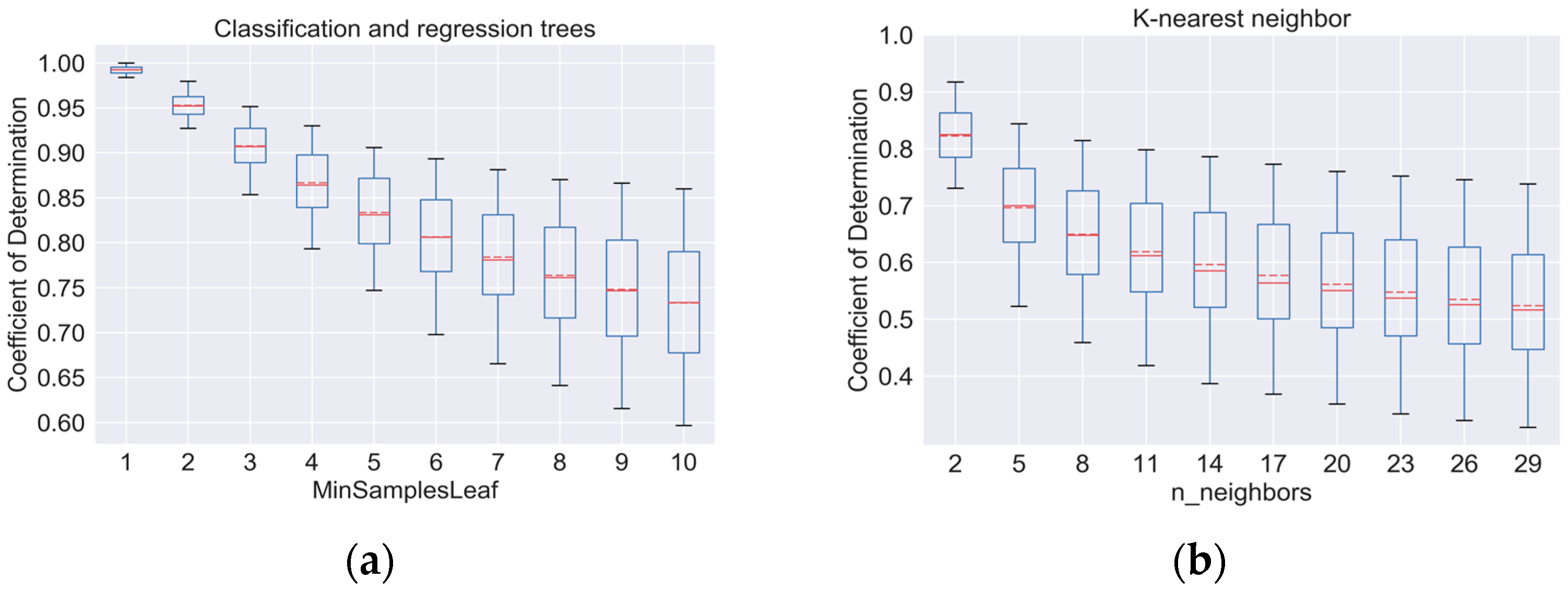
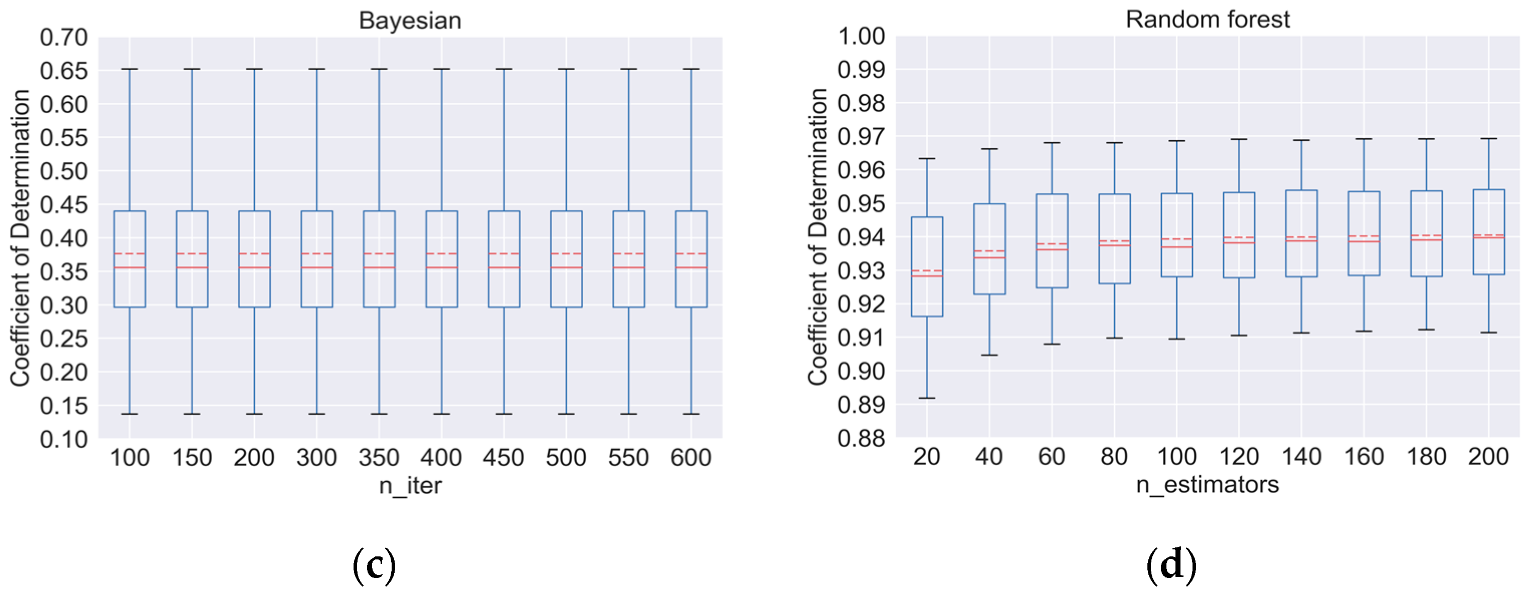
We calculated the 10-year arithmetic mean coefficients of determination (R2) of the four machine learning downscaling algorithms. Figure 3 shows R2 with different parameters of CART, KNN, BAYE and RF. It is illustrated that with the increasing of MinSamplesLeaf of CART, the R2 values decreased remarkably from nearly 1.00 to 0.73. This is similar to the R2 values of KNN, which fluctuate from 0.82 to 0.51 as n_estimators vary between 2 and 29. Both CART and KNN are vulnerable to parameter changes. On the contrary, BAYE and RF behave more stably with respect to parameter changes, indicating the notable robustness of these two methods. Additionally, compared to BAYE, RF shows outstanding performance with R2 generally greater than 0.92.
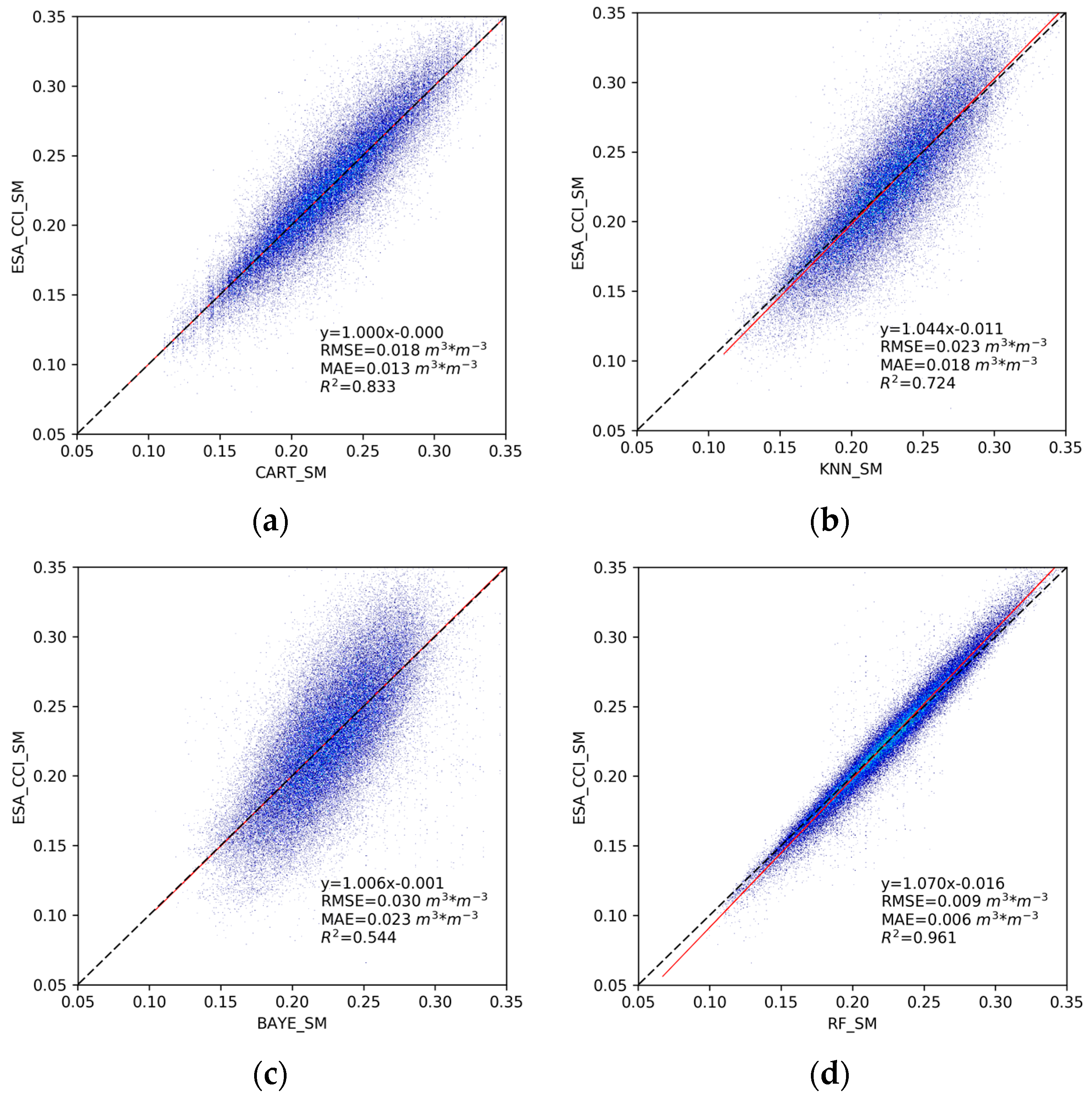
To investigate the goodness of fit between the original ESA CCI SM and CART, KNN, BAYE and RF downscaled SM (CART_SM, KNN_SM, BAYE_SM and RF_SM), we drew scatterplots and established regression correlations, as shown in in Figure 4. When the downscaled 1-km SM data were resampled to the 25-km scale, the upscaling procedure could eliminate extreme values and tended to homogenize the whole area by simple arithmetic mean. In consequence, the monthly 25-km ESA CCI SM was first regressed to 25 km other than 1 km to retain the raw regressed values. In terms of the root mean square error (RMSE), mean absolute error (MAE), and R2 (coefficient of determination), RF behaved the best with RMSE = 0.009 m3·m−3, MAE = 0.006 m3·m−3, and R2 = 0.961, followed by CART, KNN, and BAYE. In addition, considering the slope and intercept in the linear regression equation, CART produced a better fit degree with the original SM data (y = 1.000x − 0.000) than all the other algorithms. The slopes of KNN, BAYE and RF were all greater than 1.0, which indicated that the three regressions slightly underestimated the SM data during regression. Overall, it is suggested that RF and CART seemed to outperform KNN and BAYE in processing the SM data. Figure 5 shows that the ESA CCI SM and machine learning methods-processed SM had similar mean values. However, ESA CCI SM showed the largest standard deviation (0.044), followed by RF_SM (0.041) and CART_SM (0.040). BAYE_SM had the least standard deviation (0.036). Additionally, this explained the why in Figure 4 RF_SM had the largest value range and BAYE_SM had the lowest value range. The standard deviation in the error bar reflected the discretization degree of each SM dataset by calculating the average value of deviations from the average data. By contrast, RMSE expressed the degree of deviation from the ESA CCI SM value of the machine learning-regressed data.
Similarly, we analyzed the matching level between ESA CCI SM and the four algorithms regressed SM data in different months. Table 2 revealed that all the months’ SM data demonstrated an approximate 1:1 positive correlation with average slopes and interceptions ranging from 1.026 to 1.059 and −0.001 to −0.014 respectively. Moreover, the average RMSE value interval (0.018–0.022 m3·m−3) and MAE value range (0.006–0.007 m3·m−3) clarified that deviation and error between regressed values and true values were also small. However, lower R2 = 0.662 in August presented that the fitting degree of the model was not as good as for the other months. This phenomenon may result from the comprehensive impact of heavy rainfall causing a sharp rise in local SM, especially in low-lying areas, as well as high-temperature oriented sunny slopes with SM rapid evaporation, which co-contributed to comparatively uneven and irregular distribution of SM value.
4.2. Downscaled Soil Moisture
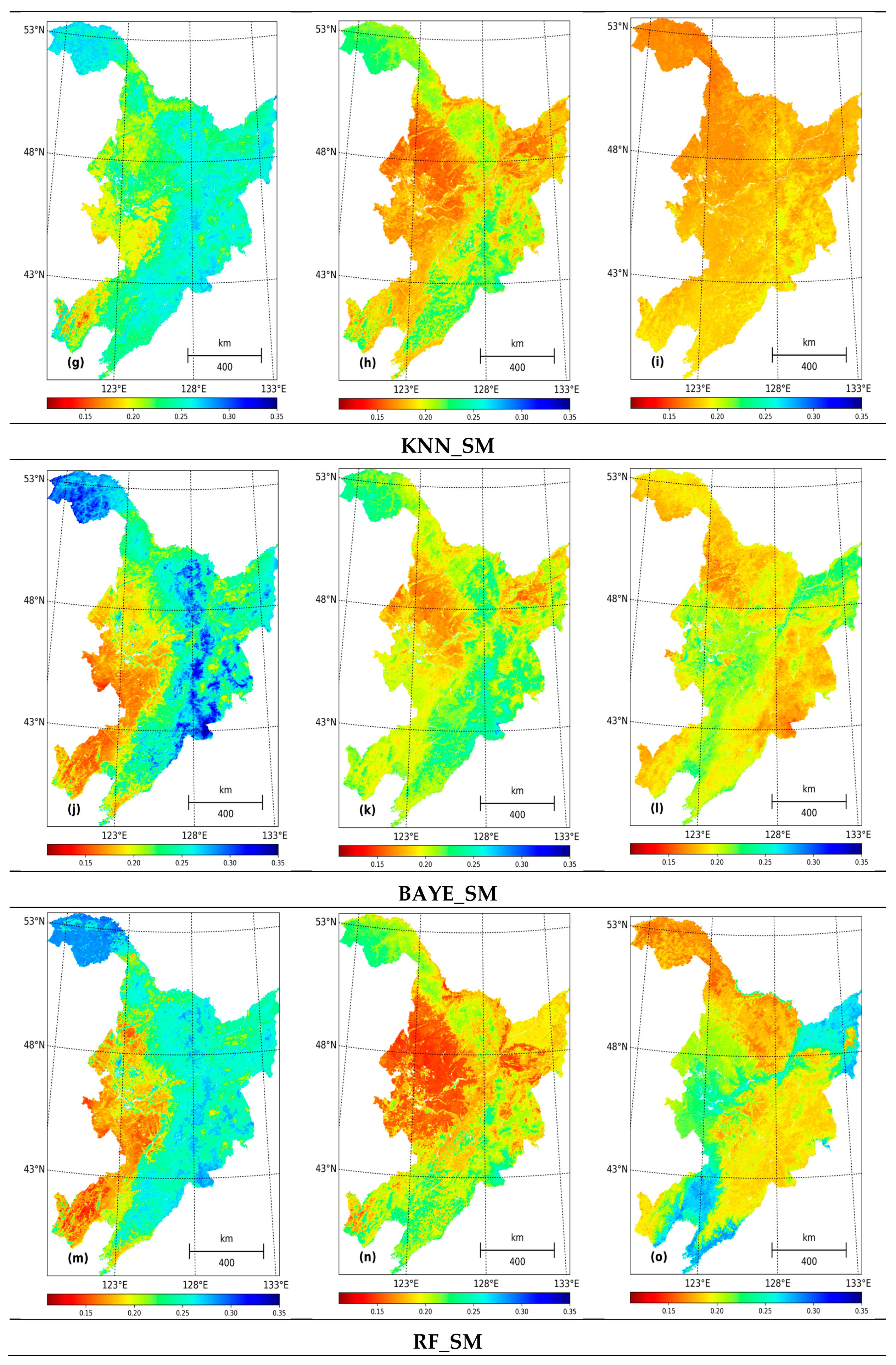
We compared the ESA CCI SM and CART, KNN, BAYE, and RF downscaled SM in April 2003, May 2009 and October 2011 in Figure 6. The CART_SM produced a similar spatial distribution pattern to ESA CCI SM in May 2009, but shows obvious differences to ESA CCI SM in the eastern, northern, and central regions of the study area in April 2003 and October 2011. In comparison, KNN_SM generally underestimated the SM value. In addition, BAYE_SM remained consistent with ESA CCI SM data in April 2003 and May 2009, but it failed to reveal high-value areas in October 2011. By contrast, both the RF_SM value range and spatial distribution present an outstanding matching degree.
4.3. Validation for In-Situ Soil Moisture
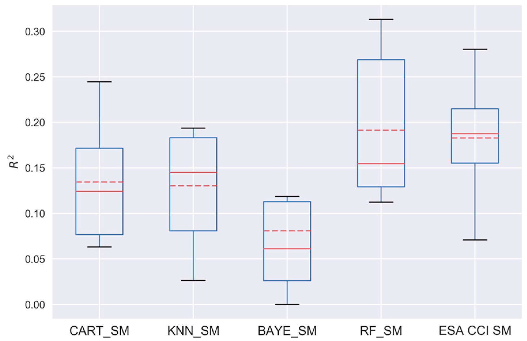
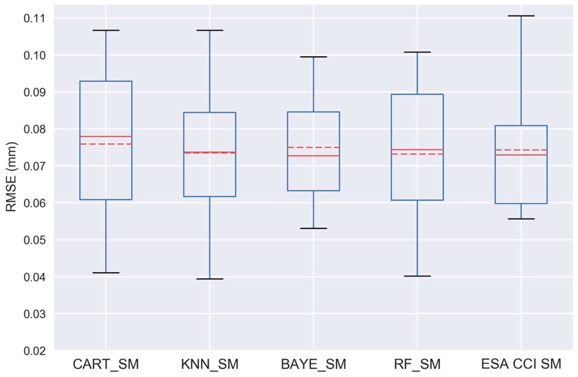
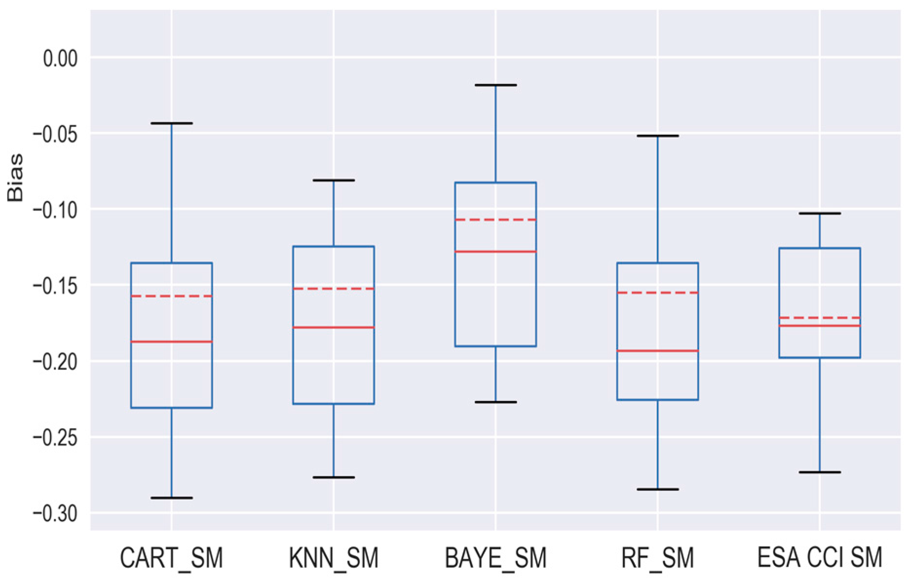
The in-situ measurements from eight sites were utilized to validate the downscaled SM data. The RMSE, MAE, Bias, and R2 were calculated. The results are shown in Table 3. We found that, in terms of R2, RF showed the superior coefficient of determination (R2 = 0.191), CART (R2 = 0.135) ranked second, followed by KNN (R2 = 0.13), and BAYE had the lowest R2 value (R2 = 0.081). In addition, BAYE performed, to some extent, better than the others in terms of Bias. Furthermore, RF and KNN revealed fairly good performance for Bias. The downscaled results produced by using the CART model had the worst accuracy of all the algorithms. The fluctuation of deviation between downscaled data and measurements was relatively small in general. Figure 7, Figure 8 and Figure 9 show the error boxplot of R2, RMSE (m3·m−3) and Bias, which are more intuitive than the numerical figures in Table 3. We can clearly see the mean, median, 75 and 25 percentiles, and maximum and minimum values of each index.
According to the analysis above, the coefficient of determination between the downscaled SM and in-situ measurements did not reach ideal accuracy. There were four specific reasons for this, which are as follows. First, the accuracy of the downscaled SM mainly relies on the accuracy of the ESA CCI SM. Table 3 shows that the average R2 value of ESA CCI SM and in-situ measurements was 0.183, which was lower than that of RF_SM. This indicates that the downscaled SM by using the RF model is more correlated to in-situ SM than the original ESA CCI SM product. Dorigo et al. [29] evaluated the ESA CCI SM product using in-situ measurements and found that RMSE varied among different networks. Furthermore, according to the validation results by using the SM networks, the integral data quality showed a decreasing tendency from 2007 to 2010. Second, ESA CCI SM acquired data in the depth range of 3–5 cm, whereas the in-situ measurements used in this study monitored SM at a depth of 10 cm. The physical factors which resulted in SM change were different at different depths. Furthermore, the sand content in soil can have an effect on microwave penetration [69], and therefore, the diversity of sand content led to different microwave penetration depth [70]. Third, the original in-situ SM data were recorded in relative humidity (%). The bulk density and field capacity data were used in unit conversion. However, their accuracies were affected by the source map, measured soil properties, and interrelations [71]. Therefore, a certain amount of error could appear during the unit conversion to volumetric water content (m3·m−3). Finally, considering the scale mismatch between the in-situ measurements and the pixels of satellite-based SM, the spatial representativeness of the point-scale in-situ measurements is not ideal for the evaluation of the coarse remote sensing SM products. Although the spatial resolution of the downscaled SM is highly improved, the grid size of the downscaled SM is still much larger than point-scale measurements.
4.4. Comparison with Precipitation Data
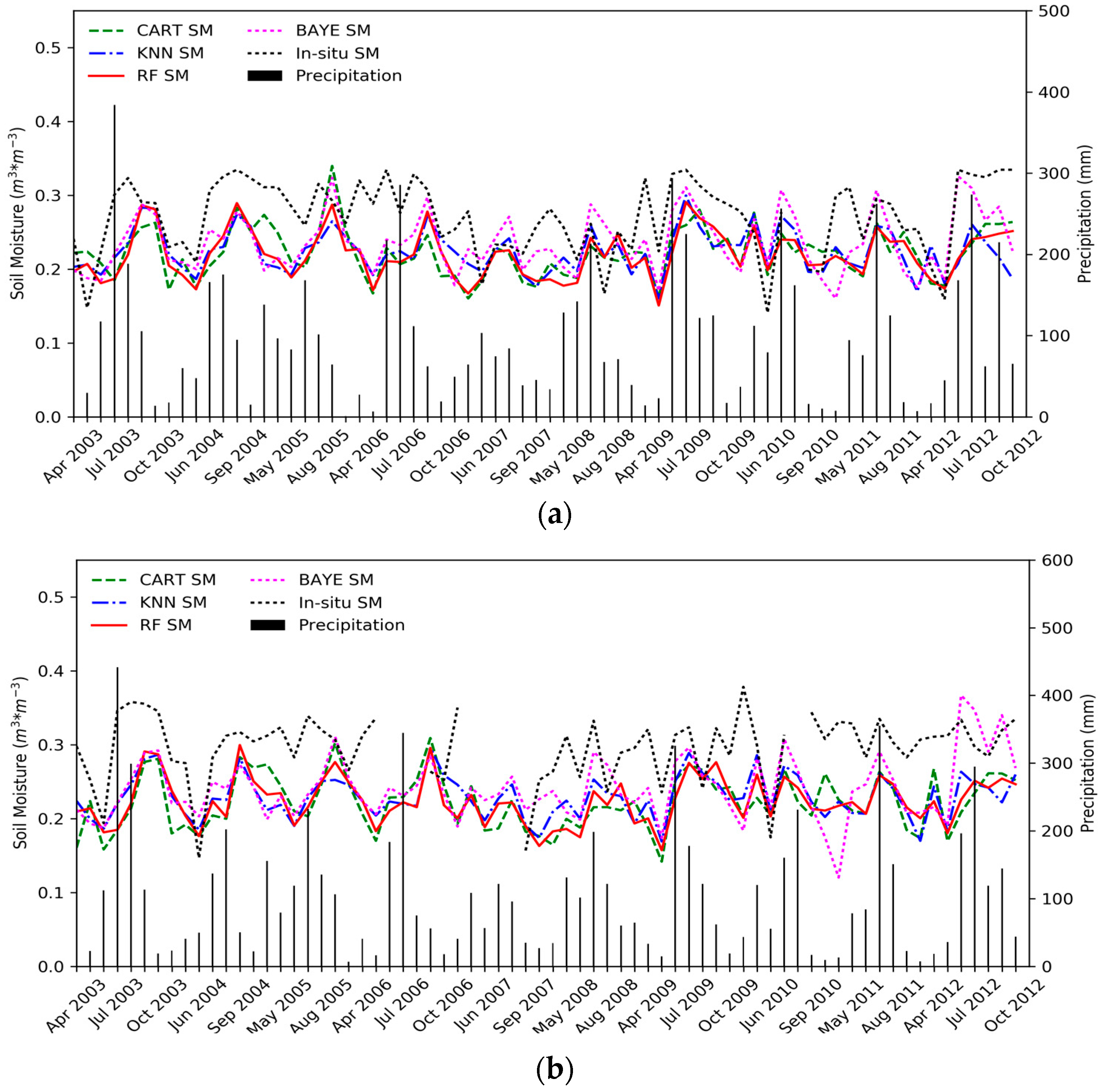
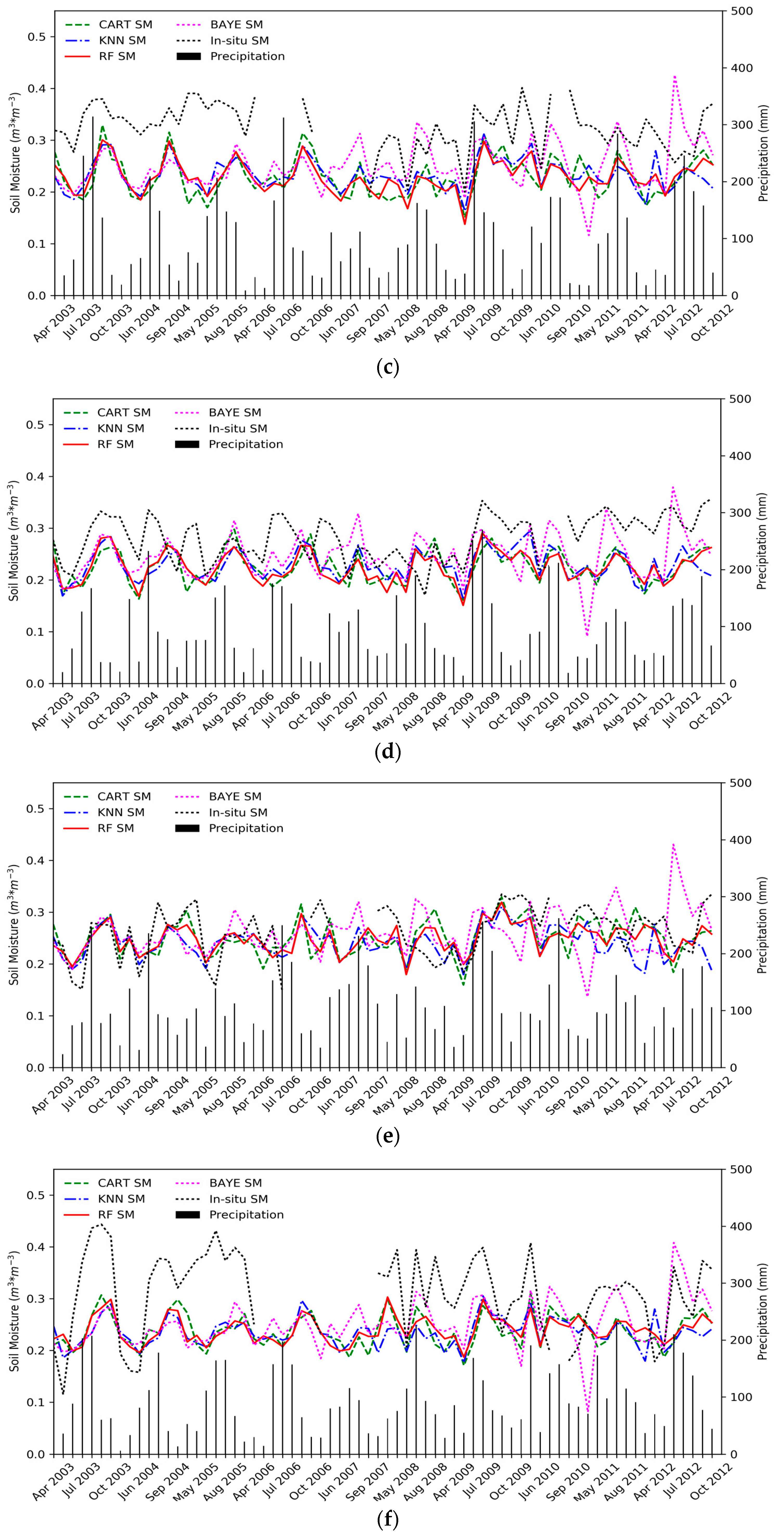
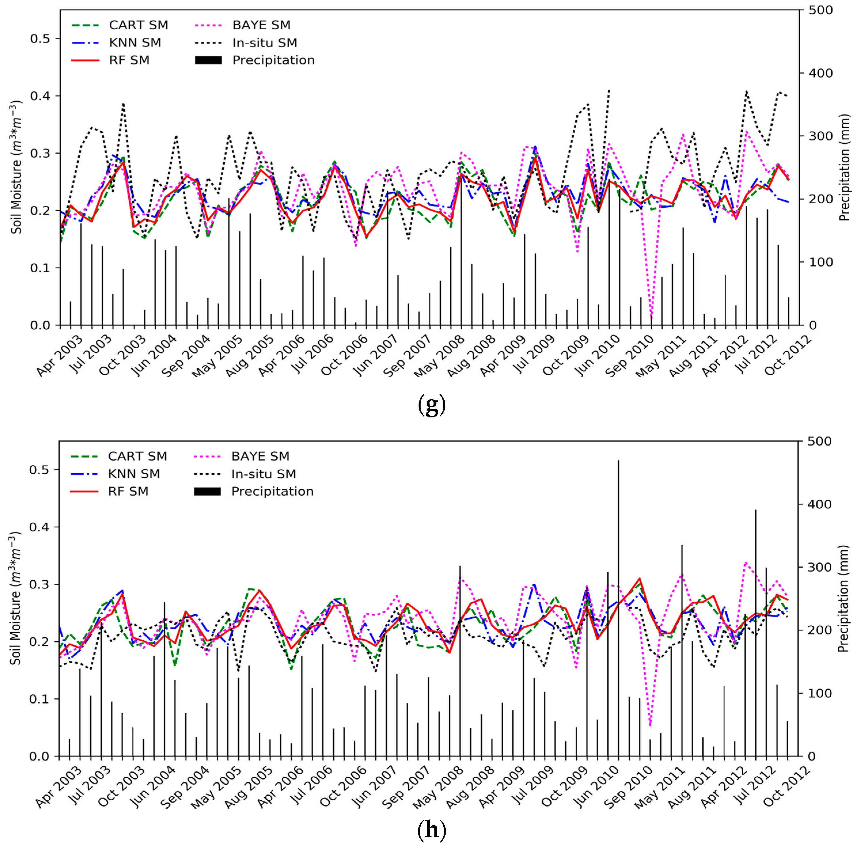
As previous studies suggested that SM could have a predominantly positive feedback on precipitation [72,73], we compared the downscaled SM, in-situ measurements, and precipitation from 2003 to 2012 in Figure 10. We utilized monthly TRMM 3B43 V7 precipitation data at a spatial resolution of 0.25° × 0.25°, which was downloaded from the official website for NASA Precipitation Measurement Missions and extracted the precipitation values via the in-situ locations.
Figure 10 shows that both SM and rainfall exhibited significant and correlative inter-annual variability. Specifically, SM showed increasing trends with the increase in precipitation in summer and declined as precipitation decreased in spring and autumn. Moreover, the precipitation is mainly concentrated in June, July and August, and the peak value of SM lagged the rainfall peak by no more than one month. When comparing the different SM, the in-situ measurements were mostly larger than the downscaled SM in Figure 10a–d,f,g, whereas the in-situ measurements were slightly smaller than the downscaled SM in Figure 10e,h. This phenomenon could probably explain the heterogeneity between SM at depths of 3–5 cm and 10 cm.
Equally, the performance of the downscaled SM was diverse among the specific methods. It is known that CART and RF are tree-based algorithms, and thus, there is a consistency in the variation tendency of the two data series. Nonetheless, CART_SM showed a few of unusual extreme values (larger peak value in October 2010 in Figure 6b and smaller valley value in August 2004 in Figure 10h than the other downscaled SM results). By contrast, RF_SM displayed relative robustness and consistency with proper values, demonstrating corresponding variation tendency and reasonable extreme values with precipitation and in-situ measurements as well. The variation tendency of KNN_SM was relatively consistent with the whole trend, but there were still some dissimilarities. For example, KNN_SM showed a peak in April 2004 in Figure 10a, whereas all the other SM results as well as precipitation present a valley at the same time. In addition, the fluctuation curve of KNN_SM was more like that of BAYE_SM; this may be because, during the regression progress, both KNN and BAYE mainly take the nearby important point values into consideration when predicting SM. BAYE_SM shows noticeably abnormal peak and valley values compared to the other downscaled SM and in-situ measurements. In general, the BAYE algorithm expressed an unstable performance in peaks and valleys during the downscaling progress.
5. Discussion
The variation of SM is a complex and synthetic process, which is impacted by numerous meteorological factors and physical aspects. Previous studies lent support to the assumption that the LST, vegetation conditions and terrain can directly affect SM [37,38,39,40,41,42,48]. However, the coarse resolution of satellite-based SM products has limited accurate regional crop yield estimation, calculation of irrigation levels, hydrothermal condition analysis and soil water holding capacity comparison. We utilized four machine learning algorithms to downscale monthly averaged ESA CCI SM from 25-km to 1-km spatial resolution by implementing LST, NDVI, surface reflection and DEM as explanatory variables. A parameter-exhaustive search method was applied to choose optimal parameters. Moreover, 1-km spatial resolution SM was validated by eight in-situ SM measurements from 2003 to 2012 to verify the quality and features of the downscaled results.
Four typical machine learning algorithms, namely BAYE, CART, KNN, and RF, were chosen to acquire fine-resolution SM imagery. An exhaustive method implemented in Python was employed to pick optimal parameters and compare the robustness of different algorithms. Moreover, these findings provide evidence that RF ranked first with stable superior performance and the highest R2, CART ranked second with R2 ranging from nearly 1.00 to 0.73, followed by KNN, and BAYE ranked last. This ranking applied equally to correlation and accuracy analysis between ESA CCI SM and the four regressed SM results. Moreover, the machine learning algorithm-regressed SM also matched quite well with ESA CCI SM monthly, except in August. This was a period when a large amount of precipitation converged on low-lying land and soil water on a sunny slope evaporated rapidly owing to a high LST. In consequence, when studying SM downscaling in summer in the future, detailed terrain attributes such as slope, aspect and elevation should be taken into account. In addition, the validation between the downscaled SM and in-situ measurements did not obtain ideal accuracy. This phenomenon could be mainly ascribed to four points: (1) The quality of the downscaled SM was based on the quality of the ESA CCI SM. Consequently, the correlation level between the in-situ measurements and downscaled SM was limited by the precision of the original data. (2) Previous studies showed that as sandy soil has massive macropores and an air–soil interface, microwave penetration depth increases with increasing soil sand content [69,70,74]. Additionally, high sand content caused multiple reflection/scattering and led to higher reflectance [74]. Hence, in theory, a diversity of sand content led to different microwave penetration depth. (3) Bulk density and field capacity data were developed by multiple pedotransfer functions, which represent regional digital soil properties [50]. However, the precision of the dataset cannot exceed the source data, including the soil map, measured soil attributes, and the linking relationship [71], and these are the sources of uncertainty. Accordingly, errors resulting from the unit conversion (from relative humidity (%) to volumetric water content (m3·m−3)) could appear. (4) The spatial representativeness of the point-scale in-situ measurements could hardly stand for the integral SM of 1 km2; namely, there is a SM value mismatch between the point-scale and 1-km-pixel scale.
Therefore, it is necessary to explore other effective validation methods to evaluate downscaled SM, objectively and effectively. Thus, considering the positive feedback relation between SM and precipitation, we tried to analyze the tendency correlation between downscaled SM, in-situ SM, and precipitation data. We found that the SM peak value lagged the rainfall peak by no more than one month, which means that precipitation can have a remarkable promotion effect on SM. Hence, SM-related physical elements could be employed in validating downscaled SM accuracy in the next study to explore multiple and efficient validation methods.
This study has attempted to downscale ESA CCI SM and evaluate the accuracy of four selected machine learning downscaling algorithms. Among the regression methods, RF_SM ranked first with preferable SM values and matching degree. BAYE_SM showed the worst accuracy, with apparent abnormal extreme values and low R2. For CART_SM and KNN_SM, the former had an advantage in correlation whereas the latter did well in data accuracy.
Additionally, the artificial neural network (ANN) is an important and rapid developing machine learning algorithm in recent years. It has been widely utilized in soil moisture downscaling [37], precipitation downscaling [75], rainfall–runoff modeling [76] and other hydrological process simulation and achieved relative good performance. Thus, we tested the performance of ANN in downscaling ESA CCI SM over Northeast China. However, comparing to the ESA CCI SM, the downscaled values lacked spatial consistency. Thus, we did not further analyze ANN downscaled product. According to our speculation, the reasons may be attributed to two aspects. First, different number and kinds of explanatory variables could result in different downscaled results by ANN. Second, heterogeneous soil attributes and study area could also lead to different downscaled outcome. The ANN is an outstanding machine learning algorithm, but it performed poorly in the experiments. We did not include the ANN in the comparison in this study, because the detailed mechanisms for the inconsistency are still not comprehensible and remain to be investigated, and the conclusions should be drawn very cautiously.
6. Conclusions
The traditional coarse spatial resolution of satellite-based SM, despite its wide coverage area, could hardly satisfy high-accuracy geological analysis requirements such as regional hydrological process analysis, crop yield estimation, and land surface evapotranspiration analogy. Moreover, it seems that a basic linear regression model and universal triangle method are vulnerable to parameter variation. To date, machine learning downscaling algorithms have been extensively utilized in regressing hydrology-related subjects of remote sensing data. Accordingly, there is an urgent need for retrieving high-resolution SM from satellite-based coarse SM images by machine learning methods and evaluating its precision.
As there is a lack of studies on multiple parameters including satellite-based SM downscaling, we implemented 1-km SM-relevant parameters to downscale 25-km ESA CCI SM by four machine learning methods (BAYE, CART, KNN and RF). From the four regression results, it could be concluded with certainty that RF_SM showed the best performance in both value accuracy and tendency variation. CART and KNN ranked second by showing their own disadvantages in data accuracy and correlation, respectively. BAYE ranked last, with significantly abnormal regression values.
This study has taken a step in the direction of comparing the capacity and suitability of different machine-learning-based algorithms in downscaling ESA CCI SM. In the future, further studies would be focused on clarifying the mechanism by which these parameters act on SM and result in its variation. This could be beneficial for the chosen explanatory variables in the downscaling process. Additionally, the attributes of the soil itself, such as sand content, parent material and organic matter content can also impact soil water holding capacity. Thus, the soil attribute data play a vital role in SM as well and could be applied to SM downscaling.
Acknowledgments
This study was jointly supported by the Geographic Resources and Ecology Knowledge Service System of China Knowledge Center for Engineering Sciences and Technology (No. CKCEST-2015-1-4), the National Special Program on Basic Science and Technology Research of China (No. 2013FY110900), the National Data Sharing Infrastructure of Earth System Science and the National Natural Science Foundation of China (41401430). We are indebted to the National Aeronautics and Space Administration and the United States Geological Survey for providing MODIS, DEM and TRMM data, European Space Agency for providing ESA CCI SM data, and China Meteorological Science Data Sharing Network for providing in-situ measurements. We also thank the National Data Sharing Infrastructure of Earth System Science for providing the boundary data of Northeast China. In addition, we appreciate the anonymous reviewers for their valuable comments and suggestions in improving this manuscript.
Author Contributions
Yangxiaoyue Liu designed the research and drafted the manuscript. Yaping Yang conceived and improved the research. Wenlong Jing reviewed the manuscript. Xiafang Yue explained the results. All authors contributed to editing manuscript and collecting data utilized in this paper.
Conflicts of Interest
The authors declare no conflict of interest.
References
- Entekhabi, D.; Rodriguez-Iturbe, I.; Bras, R.L. Variability in large-scale water balance with land surface-atmosphere interaction. J. Clim. 1992, 5, 798–813. [Google Scholar] [CrossRef]
- Drusch, M. Initializing numerical weather prediction models with satellite-derived surface soil moisture: Data assimilation experiments with ECMWF’s Integrated Forecast System and the TMI soil moisture data set. J. Geophys. Res. Atmos. 2007, 112. [Google Scholar] [CrossRef]
- Seneviratne, S.I.; Corti, T.; Davin, E.L.; Hirschi, M.; Jaeger, E.B.; Lehner, I.; Orlowsky, B.; Teuling, A.J. Investigating soil moisture—Climate interactions in a changing climate: A review. Earth Sci. Rev. 2010, 99, 125–161. [Google Scholar] [CrossRef]
- Seneviratne, S.I.; Lüthi, D.; Litschi, M.; Schär, C. Land-atmosphere coupling and climate change in Europe. Nature 2006, 443, 205–209. [Google Scholar] [CrossRef] [PubMed]
- Engman, E.T. Applications of microwave remote sensing of soil moisture for water resources and agriculture. Remote Sens. Environ. 1991, 35, 213–226. [Google Scholar] [CrossRef]
- Denmead, O.; Shaw, R.H. Availability of soil water to plants as affected by soil moisture content and meteorological conditions. Agron. J. 1962, 54, 385–390. [Google Scholar] [CrossRef]
- Jiang, Y.; Weng, Q. Estimation of hourly and daily evapotranspiration and soil moisture using downscaled LST over various urban surfaces. GISci. Remote Sens. 2017, 54, 95–117. [Google Scholar] [CrossRef]
- Dorigo, W.; Wagner, W.; Hohensinn, R.; Hahn, S.; Paulik, C.; Xaver, A.; Gruber, A.; Drusch, M.; Mecklenburg, S. The International Soil Moisture Network: A data hosting facility for global in situ soil moisture measurements. Hydrol. Earth Syst. Sci. 2011, 15, 1675–1698. [Google Scholar] [CrossRef]
- Robock, A.; Vinnikov, K.Y.; Srinivasan, G.; Entin, J.K.; Hollinger, S.E.; Speranskaya, N.A.; Liu, S.; Namkhai, A. The Global Soil Moisture Data Bank. Bull. Am. Meteorol. Soc. 2000, 81, 1281–1300. [Google Scholar] [CrossRef]
- Bitar, A.A.; Leroux, D.; Kerr, Y.H.; Merlin, O.; Richaume, P.; Sahoo, A.; Wood, E.F. Evaluation of SMOS Soil Moisture Products Over Continental U.S. Using the SCAN/SNOTEL Network. IEEE Trans. Geosci. Remote Sens. 2012, 50, 1572–1586. [Google Scholar] [CrossRef] [Green Version]
- Xu, B.; Li, J. A methodology to estimate representativeness of LAI station observation for validation: A case study with Chinese Ecosystem Research Network (CERN) in situ data. In Proceedings of the SPIE Asia Pacific Remote Sensing, Beijing, China, 27–31 October 2014. [Google Scholar]
- Paulik, C.; Dorigo, W.; Wagner, W.; Kidd, R. Validation of the ASCAT Soil Water Index using in situ data from the International Soil Moisture Network. Int. J. Appl. Earth Obs. Geoinf. 2014, 30, 1–8. [Google Scholar] [CrossRef]
- Murray, S.J.; Foster, P.N.; Prentice, I.C. Evaluation of global continental hydrology as simulated by the Land-surface processes and exchanges dynamic global vegetation model. Hydrol. Earth Syst. Sci. 2011, 15, 91–105. [Google Scholar] [CrossRef]
- Fu, B.; Li, S.; Yu, X.; Yang, P.; Yu, G.; Feng, R.; Zhuang, X. Chinese ecosystem research network: Progress and perspectives. Ecol. Complex. 2010, 7, 225–233. [Google Scholar] [CrossRef]
- Dorigo, W.; Xaver, A.; Vreugdenhil, M.; Gruber, A.; Hegyiová, A.; Sanchis-Dufau, A.; Zamojski, D.; Cordes, C.; Wagner, W.; Drusch, M.; et al. Global automated quality control of in situ soil moisture data from the International Soil Moisture Network. Vadose Zone J. 2013, 12. [Google Scholar] [CrossRef]
- Albergel, C.; de Rosnay, P.; Gruhier, C.; Muñoz-Sabater, J.; Hasenauer, S.; Isaksen, L.; Kerr, Y.; Wagner, W. Evaluation of remotely sensed and modelled soil moisture products using global ground-based in situ observations. Remote Sens. Environ. 2012, 118, 215–226. [Google Scholar] [CrossRef]
- Dorigo, W.; Oevelen, P.; Wagner, W.; Drusch, M.; Mecklenburg, S.; Robock, A.; Jackson, T. A new international network for in situ soil moisture data. Eos Trans. Am. Geophys. Union 2011, 92, 141–142. [Google Scholar] [CrossRef]
- Gruber, A.; Dorigo, W.; Zwieback, S.; Xaver, A.; Wagner, W. Characterizing coarse-scale representativeness of in situ soil moisture measurements from the International Soil Moisture Network. Vadose Zone J. 2013, 12. [Google Scholar] [CrossRef]
- Wang, Y.; Shao, M.A.; Liu, Z. Large-scale spatial variability of dried soil layers and related factors across the entire Loess Plateau of China. Geoderma 2010, 159, 99–108. [Google Scholar] [CrossRef]
- Feng, X.; Li, J.; Cheng, W.; Fu, B.; Wang, Y.; Lü, Y.; Shao, M. Evaluation of AMSR-E retrieval by detecting soil moisture decrease following massive dryland re-vegetation in the Loess Plateau, China. Remote Sens. Environ. 2017, 196, 253–264. [Google Scholar] [CrossRef]
- Lobl, E. Joint advanced microwave scanning radiometer (AMSR) science team meeting. Earth Obs. 2001, 13, 3–9. [Google Scholar]
- Li, L.; Njoku, E.G.; Im, E.; Chang, P.S.; Germain, K.S. A preliminary survey of radio-frequency interference over the US in Aqua AMSR-E data. IEEE Trans. Geosci. Remote Sens. 2004, 42, 380–390. [Google Scholar] [CrossRef]
- Kerr, Y.H.; Waldteufel, P.; Wigneron, J.-P.; Martinuzzi, J.; Font, J.; Berger, M. Soil moisture retrieval from space: The Soil Moisture and Ocean Salinity (SMOS) mission. IEEE Trans. Geosci. Remote Sens. 2001, 39, 1729–1735. [Google Scholar] [CrossRef]
- Gaiser, P.W.; St. Germain, K.M.; Twarog, E.M.; Poe, G.A.; Purdy, W.; Richardson, D.; Grossman, W.; Jones, W.L.; Spencer, D.; Golba, G.; et al. The WindSat spaceborne polarimetric microwave radiometer: Sensor description and early orbit performance. IEEE Trans. Geosci. Remote Sens. 2004, 42, 2347–2361. [Google Scholar] [CrossRef]
- Moran, M.S.; Peters-Lidard, C.D.; Watts, J.M.; McElroy, S. Estimating soil moisture at the watershed scale with satellite-based radar and land surface models. Can. J. Remote Sens. 2004, 30, 805–826. [Google Scholar] [CrossRef]
- Wagner, W.; Lemoine, G.; Rott, H. A method for estimating soil moisture from ERS scatterometer and soil data. Remote Sens. Environ. 1999, 70, 191–207. [Google Scholar] [CrossRef]
- Paloscia, S.; Pettinato, S.; Santi, E.; Notarnicola, C.; Pasolli, L.; Reppucci, A. Soil moisture mapping using Sentinel-1 images: Algorithm and preliminary validation. Remote Sens. Environ. 2013, 134, 234–248. [Google Scholar] [CrossRef]
- Entekhabi, D.; Njoku, E.G.; O’Neill, P.E.; Kellogg, K.H.; Crow, W.T.; Edelstein, W.N.; Entin, J.K.; Goodman, S.D.; Jackson, T.J.; Johnson, J.; et al. The soil moisture active passive (SMAP) mission. Proc. IEEE 2010, 98, 704–716. [Google Scholar] [CrossRef]
- Dorigo, W.; Gruber, A.; de Jeu, R.; Wagner, W.; Stacke, T.; Loew, A.; Albergel, C.; Brocca, L.; Chung, D.; Parinussa, R.; et al. Evaluation of the ESA CCI soil moisture product using ground-based observations. Remote Sens. Environ. 2015, 162, 380–395. [Google Scholar] [CrossRef]
- Shuttleworth, J.; Rosolem, R.; Zreda, M.; Franz, T. The COsmic-ray Soil Moisture Interaction Code (COSMIC) for use in data assimilation. Hydrol. Earth Syst. Sci. 2013, 17, 3205–3217. [Google Scholar] [CrossRef]
- Djamai, N.; Magagi, R.; Goïta, K.; Merlin, O.; Kerr, Y.; Roy, A. A combination of DISPATCH downscaling algorithm with CLASS land surface scheme for soil moisture estimation at fine scale during cloudy days. Remote Sens. Environ. 2016, 184, 1–14. [Google Scholar] [CrossRef]
- Mallick, K.; Bhattacharya, B.K.; Patel, N. Estimating volumetric surface moisture content for cropped soils using a soil wetness index based on surface temperature and NDVI. Agric. For. Meteorol. 2009, 149, 1327–1342. [Google Scholar] [CrossRef]
- Sandholt, I.; Rasmussen, K.; Andersen, J. A simple interpretation of the surface temperature/vegetation index space for assessment of surface moisture status. Remote Sens. Environ. 2002, 79, 213–224. [Google Scholar] [CrossRef]
- Fang, B.; Lakshmi, V.; Bindlish, R.; Jackson, T.J.; Cosh, M.; Basara, J. Passive microwave soil moisture downscaling using vegetation index and skin surface temperature. Vadose Zone J. 2013, 12. [Google Scholar] [CrossRef]
- Piles, M.; Camps, A.; Vall-Llossera, M.; Corbella, I.; Panciera, R.; Rudiger, C.; Kerr, Y.H.; Walker, J. Downscaling SMOS-derived soil moisture using MODIS visible/infrared data. IEEE Trans. Geosci. Remote Sens. 2011, 49, 3156–3166. [Google Scholar] [CrossRef]
- Justice, C.O.; Vermote, E.; Townshend, J.R.G.; Defries, R.; Roy, D.P.; Hall, D.K.; Salomonson, V.V.; Privette, J.L.; Riggs, G.; Strahler, A.; et al. The Moderate Resolution Imaging Spectroradiometer (MODIS): Land remote sensing for global change research. IEEE Trans. Geosci. Remote Sens. 1998, 36, 1228–1249. [Google Scholar] [CrossRef]
- Srivastava, P.K.; Han, D.; Ramirez, M.R.; Islam, T. Machine Learning Techniques for Downscaling SMOS Satellite Soil Moisture Using MODIS Land Surface Temperature for Hydrological Application. Water Resour. Manag. 2013, 27, 3127–3144. [Google Scholar] [CrossRef]
- Peng, J.; Loew, A.; Zhang, S.; Wang, J.; Niesel, J. Spatial downscaling of satellite soil moisture data using a vegetation temperature condition index. IEEE Trans. Geosci. Remote Sens. 2016, 54, 558–566. [Google Scholar] [CrossRef]
- Jing, W.; Yang, Y.; Yue, X.; Zhao, X. A Comparison of Different Regression Algorithms for Downscaling Monthly Satellite-Based Precipitation over North China. Remote Sens. 2016, 8, 835. [Google Scholar] [CrossRef]
- Huete, A.R. A soil-adjusted vegetation index (SAVI). Remote Sens. Environ. 1988, 25, 295–309. [Google Scholar] [CrossRef]
- Merlin, O.; Walker, J.P.; Chehbouni, A.; Kerr, Y. Towards deterministic downscaling of SMOS soil moisture using MODIS derived soil evaporative efficiency. Remote Sens. Environ. 2008, 112, 3935–3946. [Google Scholar] [CrossRef] [Green Version]
- Merlin, O.; Al Bitar, A.; Walker, J.P.; Kerr, Y. An improved algorithm for disaggregating microwave-derived soil moisture based on red, near-infrared and thermal-infrared data. Remote Sens. Environ. 2010, 114, 2305–2316. [Google Scholar] [CrossRef] [Green Version]
- Moore, I.; Burch, G.; Mackenzie, D. Topographic effects on the distribution of surface soil water and the location of ephemeral gullies. Trans. ASAE 1988, 31, 1098–1107. [Google Scholar] [CrossRef]
- Samworth, R.J. Optimal weighted nearest neighbour classifiers. Ann. Stat. 2012, 40, 2733–2763. [Google Scholar] [CrossRef]
- Zellner, A. On assessing prior distributions and Bayesian regression analysis with G-prior distributions. Bayesian Inference Decis. Tech. 1986, 6, 233–243. [Google Scholar]
- Breiman, L.I.; Friedman, J.H.; Olshen, R.A.; Stone, C.J. Classification and Regression Trees (CART). Biometrics 1984, 40, 358. [Google Scholar]
- Svetnik, V.; Liaw, A.; Tong, C.; Culberson, J.C.; Sheridan, R.P.; Feuston, B.P. Random Forest: A Classification and Regression Tool for Compound Classification and QSAR Modeling. J. Chem. Inf. Comput. Sci. 2003, 43, 1947–1958. [Google Scholar] [CrossRef] [PubMed]
- Carlson, T.N.; Gillies, R.R.; Perry, E.M. A method to make use of thermal infrared temperature and NDVI measurements to infer surface soil water content and fractional vegetation cover. Remote Sens. Rev. 1994, 9, 161–173. [Google Scholar] [CrossRef]
- Wei, S.U.; De-Yong, Y.U.; Sun, Z.P.; Zhan, J.G.; Liu, X.X.; Qian, L. Vegetation changes in the agricultural-pastoral areas of northern China from 2001 to 2013. J. Integr. Agric. 2016, 15, 1145–1156. [Google Scholar]
- Dai, Y.; Shangguan, W.; Duan, Q.; Liu, B.; Fu, S.; Niu, G. Development of a China Dataset of Soil Hydraulic Parameters Using Pedotransfer Functions for Land Surface Modeling. J. Hydrometeorol. 2013, 14, 869–887. [Google Scholar] [CrossRef]
- Shangguan, W.; Dai, Y.; Liu, B.; Zhu, A.; Duan, Q.; Wu, L.; Ji, D.; Ye, A.; Yuan, H.; Zhang, Q. A China data set of soil properties for land surface modeling. J. Adv. Model. Earth Syst. 2013, 5, 212–224. [Google Scholar] [CrossRef]
- Bontemps, S.; Defourny, P.; Radoux, J.; van Bogaert, E.; Lamarche, C.; Achard, F.; Mayaux, P.; Boettcher, M.; Brockmann, C.; Kirches, G. Consistent global land cover maps for climate modelling communities: Current achievements of the ESA’s land cover CCI. In Proceedings of the ESA Living Planet Symposium, Edimburgh, UK, 9–13 September 2013. [Google Scholar]
- Hollmann, R.; Merchant, C.J.; Saunders, R.; Downy, C.; Buchwitz, M.; Cazenave, A.; Chuvieco, E.; Defourny, P.; de Leeuw, G.; Forsberg, R.; et al. The ESA climate change initiative: Satellite data records for essential climate variables. Bull. Am. Meteorol. Soc. 2013, 94, 1541–1552. [Google Scholar] [CrossRef]
- McNally, A.; Shukla, S.; Arsenault, K.R.; Wang, S.; Peters-Lidard, C.D.; Verdin, J.P. Evaluating ESA CCI soil moisture in East Africa. Int. J. Appl. Earth Obs. Geoinf. 2016, 48, 96–109. [Google Scholar] [CrossRef]
- Justice, C.O.; Townshend, J.R.G.; Vermote, E.F.; Masuoka, E.; Wolfe, R.E.; Saleous, N.; Roy, D.P.; Morisette, J.T. An overview of MODIS Land data processing and product status. Remote Sens. Environ. 2002, 83, 3–15. [Google Scholar] [CrossRef]
- Rabus, B.; Eineder, M.; Roth, A.; Bamler, R. The shuttle radar topography mission—A new class of digital elevation models acquired by spaceborne radar. ISPRS J. Photogramm. Remote Sens. 2003, 57, 241–262. [Google Scholar] [CrossRef]
- Huffman, G.J.; Adler, R.F.; Bolvin, D.T.; Nelkin, E.J. The TRMM Multi-Satellite Precipitation Analysis (TMPA). J. Hydrometeorol. 2007, 90, 237–247. [Google Scholar]
- Western, A.; Grayson, R. Soil moisture and runoff processes at Tarrawarra. Spat. Patterns Catchment Hydrol. Obs. Model. 2000, 209–246. [Google Scholar]
- Western, A.W.; Grayson, R.B.; Blöschl, G. Scaling of soil moisture: A hydrologic perspective. Annu. Rev. Earth Planet. Sci. 2002, 8, 149–180. [Google Scholar] [CrossRef]
- Burrows, W.R.; Benjamin, M.; Beauchamp, S.; Lord, E.R.; McCollor, D.; Thomson, B. CART decision-tree statistical analysis and prediction of summer season maximum surface ozone for the Vancouver, Montreal, and Atlantic regions of Canada. J. Appl. Meteorol. 1995, 34, 1848–1862. [Google Scholar] [CrossRef]
- Westreich, D.; Lessler, J.; Funk, M.J. Propensity score estimation: Neural networks, support vector machines, decision trees (CART), and meta-classifiers as alternatives to logistic regression. J. Clin. Epidemiol. 2010, 63, 826–833. [Google Scholar] [CrossRef] [PubMed]
- Yu, C.; Ooi, B.C.; Tan, K.-L.; Jagadish, H. Indexing the distance: An efficient method to knn processing. In Proceedings of the 27th International Conference on Very Large Data Bases, Roma, Italy, 11–14 September 2001. [Google Scholar]
- Drummond, A.J.; Rambaut, A. BEAST: Bayesian evolutionary analysis by sampling trees. BMC Evol. Biol. 2007, 7, 214. [Google Scholar] [CrossRef] [PubMed] [Green Version]
- Breiman, L. Random forests. Mach. Learn. 2001, 45, 5–32. [Google Scholar] [CrossRef]
- Liaw, A.; Wiener, M. Classification and regression by randomForest. R News 2002, 2, 18–22. [Google Scholar]
- Pal, M. Random forest classifier for remote sensing classification. Int. J. Remote Sens. 2005, 26, 217–222. [Google Scholar] [CrossRef]
- Pedregosa, F.; Varoquaux, G.; Gramfort, A.; Michel, V.; Thirion, B.; Grisel, O.; Blondel, M.; Prettenhofer, P.; Weiss, R.; Dubourg, V.; et al. Scikit-learn: Machine learning in Python. J. Mach. Learn. Res. 2011, 12, 2825–2830. [Google Scholar]
- Abraham, A.; Pedregosa, F.; Eickenberg, M.; Gervais, P.; Mueller, A.; Kossaifi, J.; Gramfort, A.; Thirion, B.; Varoquaux, G. Machine learning for neuroimaging with scikit-learn. Front. Neuroinform. 2014, 8, 14. [Google Scholar] [CrossRef] [PubMed] [Green Version]
- Owe, M.; Van de Griend, A.A. Comparison of soil moisture penetration depths for several bare soils at two microwave frequencies and implications for remote sensing. Water Resour. Res. 1998, 34, 2319–2327. [Google Scholar] [CrossRef] [Green Version]
- Casa, R.; Castaldi, F.; Pascucci, S.; Palombo, A.; Pignatti, S. A comparison of sensor resolution and calibration strategies for soil texture estimation from hyperspectral remote sensing. Geoderma 2013, 197–198, 17–26. [Google Scholar] [CrossRef]
- Shangguan, W.; Dai, Y.; Liu, B.; Ye, A.; Yuan, H. A soil particle-size distribution dataset for regional land and climate modelling in China. Geoderma 2012, 171–172, 85–91. [Google Scholar] [CrossRef]
- Hohenegger, C.; Brockhaus, P.; Bretherton, C.S.; Schär, C. The soil moisture—Precipitation feedback in simulations with explicit and parameterized convection. J. Clim. 2009, 22, 5003–5020. [Google Scholar] [CrossRef]
- Wagner, W.; Scipal, K.; Pathe, C.; Gerten, D.; Lucht, W.; Rudolf, B. Evaluation of the agreement between the first global remotely sensed soil moisture data with model and precipitation data. J. Geophys. Res. Atmos. 2003, 108. [Google Scholar] [CrossRef]
- Sawut, M.; Ghulam, A.; Tiyip, T.; Zhang, Y.J.; Ding, J.L.; Zhang, F.; Maimaitiyiming, M. Estimating soil sand content using thermal infrared spectra in arid lands. Int. J. Appl. Earth Obs. Geoinf. 2014, 33, 203–210. [Google Scholar] [CrossRef]
- Hoai, N.D.; Udo, K.; Mano, A. Downscaling Global Weather Forecast Outputs Using ANN for Flood Prediction. J. Appl. Math. 2011, 2011, 223–236. [Google Scholar]
- Hsu, K.; Lin, X.; Gupta, H.V.; Sorooshian, S. Artificial Neural Network Modeling of the Rainfall-Runoff Process. Water Resour. Res. 2010, 31, 2517–2530. [Google Scholar] [CrossRef]
Figure 1.
Distribution of soil moisture (SM) stations, elevation and grid cells of the European Space Agency Climate Change Initiative (ESA CCI) SM in Northeast China.
Figure 1.
Distribution of soil moisture (SM) stations, elevation and grid cells of the European Space Agency Climate Change Initiative (ESA CCI) SM in Northeast China.

Figure 2.
Specific procedures of relevant data processing and ESA CCI SM downscaling.
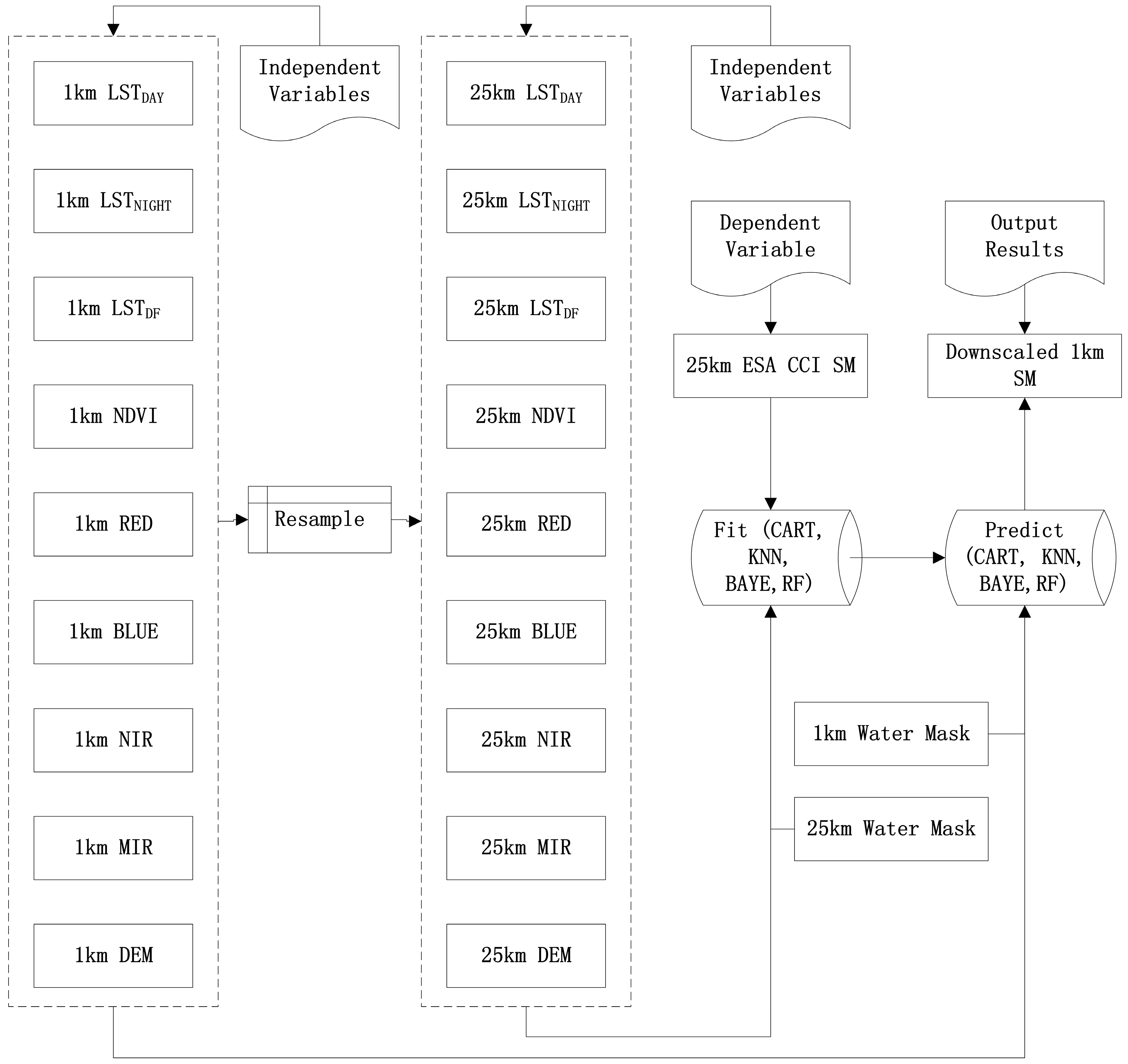
Figure 3.
Variations of coefficient of determination with different selected parameters of: (a) classification and regression trees; (b) K-nearest neighbors; (c) Bayesian; and (d) random forest.
Figure 3.
Variations of coefficient of determination with different selected parameters of: (a) classification and regression trees; (b) K-nearest neighbors; (c) Bayesian; and (d) random forest.


Figure 4.
Scatterplots, linear regression equations, RMSEs, MAEs and R2 between ESA CCI SM and: (a) CART_SM; (b) KNN_SM; (c) BAYE_SM; and (d) RF_SM.
Figure 4.
Scatterplots, linear regression equations, RMSEs, MAEs and R2 between ESA CCI SM and: (a) CART_SM; (b) KNN_SM; (c) BAYE_SM; and (d) RF_SM.

Figure 5.
Comparison of ESA CCI SM, CART_SM, KNN_SM, BAYE_SM and RF_SM by error bars.
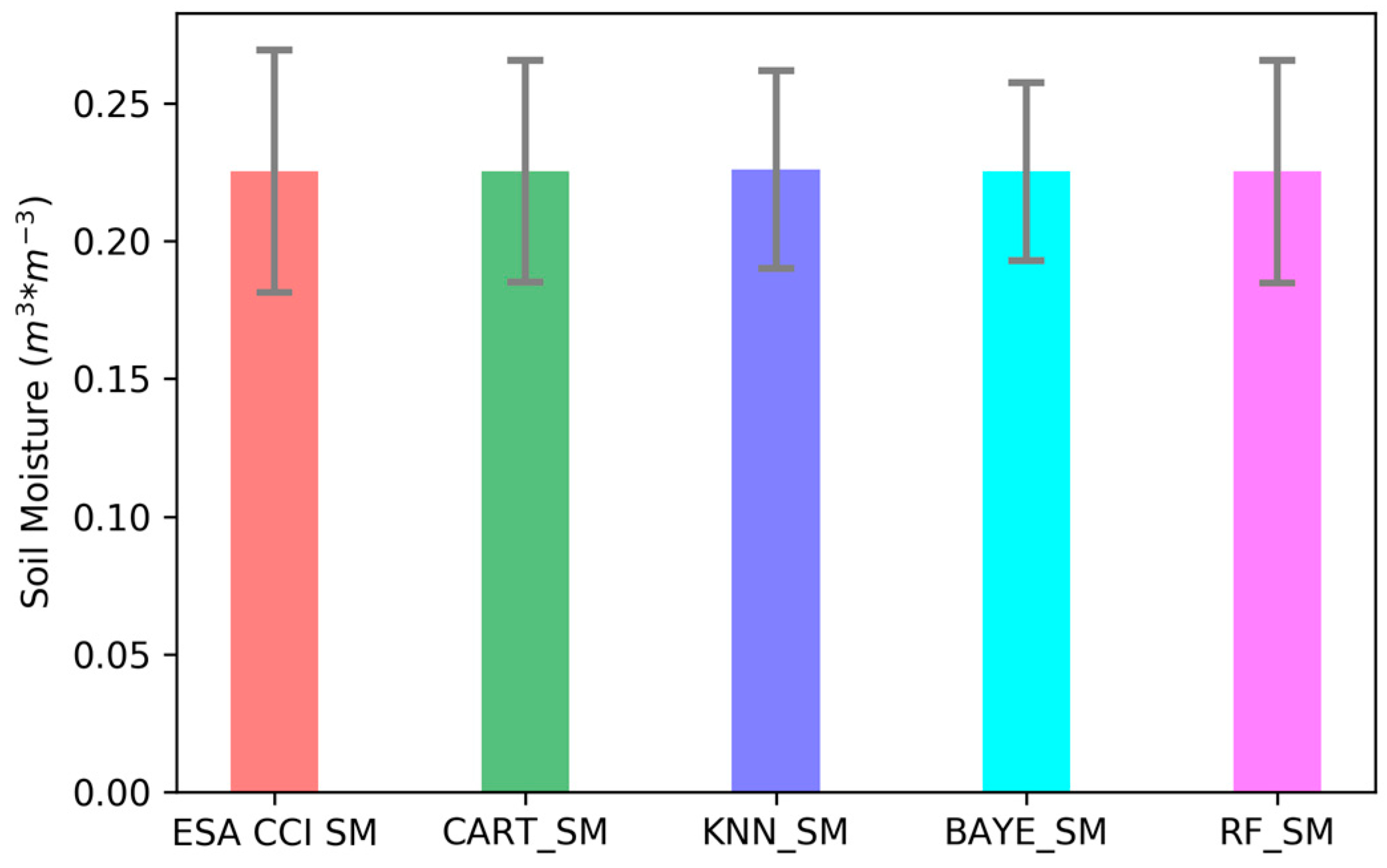
Figure 6.
Comparison of ESA CCI SM and CART_SM, KNN_SM, BAYE_SM, RF_SM in April 2003, May 2009 and October 2011. (a--c) are ESA CCI SM in April 2003, May 2009 and October 2011; (d--f) are CART_SM in April 2003, May 2009 and October 2011; (g--i) are KNN_SM in April 2003, May 2009 and October 2011; (j--l) are BAYE_SM in April 2003, May 2009 and October 2011; (m--o) are RF_SM in April 2003, May 2009 and October 2011.
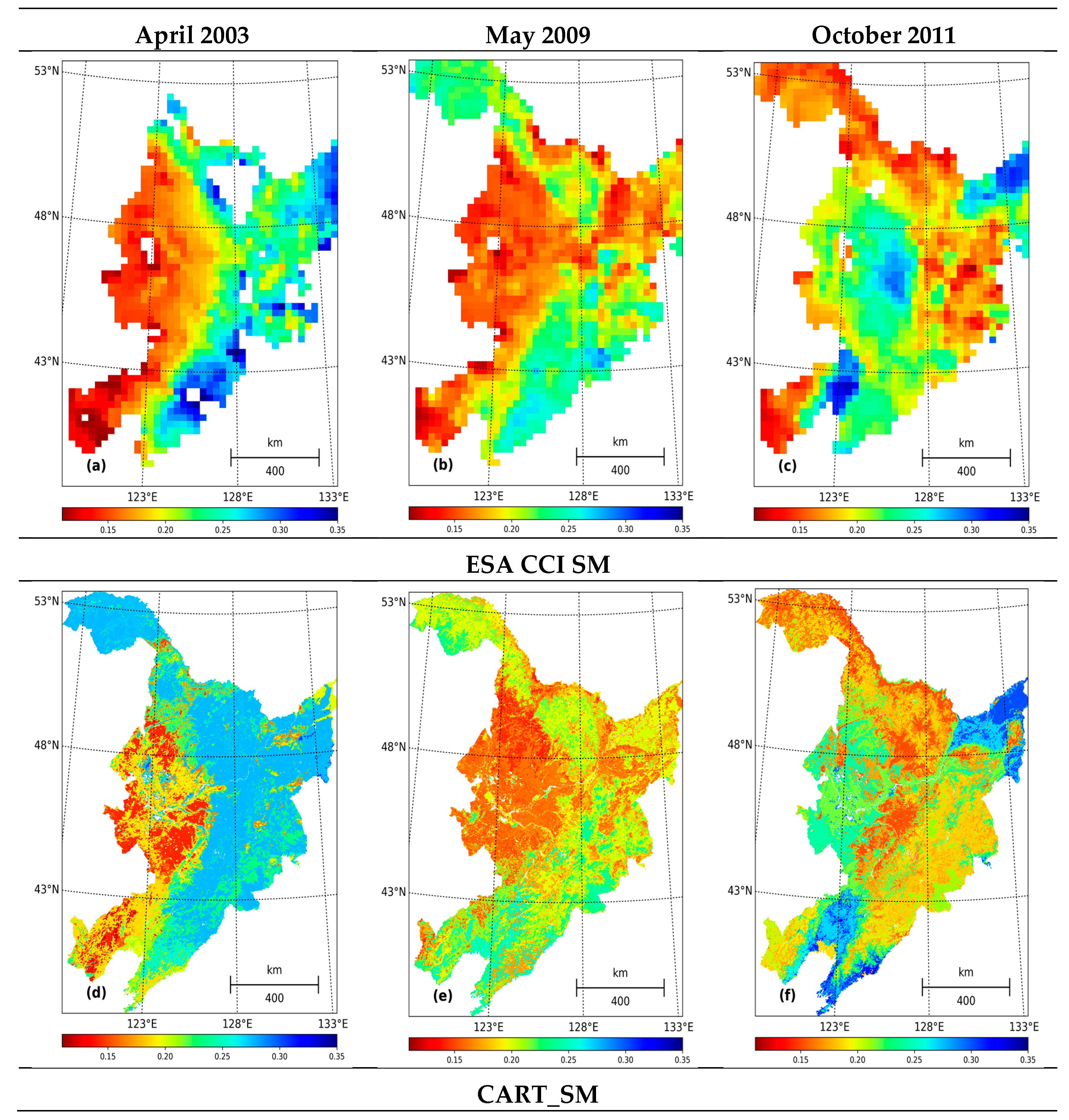

Figure 7.
Box plot of R2.

Figure 8.
Box plot of RMSE (m3·m−3).

Figure 9.
Box plot of Bias.

Figure 10.
Comparison of the four machine learning downscaled SM, in-situ measurements and precipitation from 2003 to 2012 in unfrozen seasons. (a−h) stand for the comparison in in-situ 1, 2, 3, 4, 5, 6, 7, 8 respectively.
Figure 10.
Comparison of the four machine learning downscaled SM, in-situ measurements and precipitation from 2003 to 2012 in unfrozen seasons. (a−h) stand for the comparison in in-situ 1, 2, 3, 4, 5, 6, 7, 8 respectively.


Table 1.
Parameter ranges of classification and regression trees (CART), k-nearest neighbor (KNN), Bayesian (BAYE) and random forest (RF) algorithms.
Table 1.
Parameter ranges of classification and regression trees (CART), k-nearest neighbor (KNN), Bayesian (BAYE) and random forest (RF) algorithms.
| Algorithm | Parameter Name | Parameter Meaning | Value Ranges |
|---|---|---|---|
| CART | MinSamplesLeaf | The minimum sample number to split internal node. (default = 2) | 1, 2, 3, 4, 5, 6, 7, 8, 9, 10 |
| KNN | n_neighbors | Used neighbor number. (default = 5) | 2, 5, 8, 11, 14, 17, 20, 23, 26, 29 |
| BAYE | n_iter | Maximal iteration times. (default = 300) | 100, 150, 200, 300, 350, 400, 450, 500, 550, 600 |
| RF | n_estimators | Trees in the forest. (default = 10) | 20, 40, 60, 80, 100, 120, 140, 160, 180, 200 |
Table 2.
Monthly slope, interception, RMSE, MAE and R2 between ESA CCI SM and the four algorithms regressed data.
Table 2.
Monthly slope, interception, RMSE, MAE and R2 between ESA CCI SM and the four algorithms regressed data.
| Month | Method | CART | KNN | BAYE | RF | Average |
|---|---|---|---|---|---|---|
| pril | Slope | 1 | 1.049 | 1.009 | 1.074 | 1.033 |
| Interception | 0 | −0.011 | −0.002 | −0.015 | −0.007 | |
| RMSE | 0.018 | 0.024 | 0.034 | 0.01 | 0.022 | |
| MAE | 0.012 | 0.018 | 0.026 | 0.007 | 0.016 | |
| R2 | 0.847 | 0.715 | 0.437 | 0.959 | 0.74 | |
| May | Slope | 1 | 1.041 | 1.005 | 1.059 | 1.026 |
| Interception | 0 | −0.009 | −0.001 | −0.012 | −0.001 | |
| RMSE | 0.017 | 0.022 | 0.029 | 0.009 | 0.019 | |
| MAE | 0.013 | 0.016 | 0.022 | 0.006 | 0.014 | |
| R2 | 0.849 | 0.762 | 0.575 | 0.964 | 0.79 | |
| June | Slope | 1 | 1.038 | 1.005 | 1.075 | 1.03 |
| Interception | 0 | −0.009 | −0.001 | −0.016 | −0.007 | |
| RMSE | 0.017 | 0.022 | 0.026 | 0.008 | 0.018 | |
| MAE | 0.013 | 0.017 | 0.02 | 0.006 | 0.014 | |
| R2 | 0.815 | 0.7 | 0.583 | 0.959 | 0.764 | |
| July | Slope | 1 | 1.056 | 1.006 | 1.091 | 1.038 |
| Interception | 0 | −0.014 | −0.001 | −0.022 | −0.009 | |
| RMSE | 0.019 | 0.024 | 0.027 | 0.009 | 0.02 | |
| MAE | 0.014 | 0.018 | 0.021 | 0.007 | 0.015 | |
| R2 | 0.777 | 0.641 | 0.537 | 0.954 | 0.727 | |
| August | Slope | 1 | 1.108 | 1.012 | 1.116 | 1.059 |
| Interception | 0 | −0.026 | −0.003 | −0.028 | −0.014 | |
| RMSE | 0.017 | 0.022 | 0.027 | 0.009 | 0.019 | |
| MAE | 0.013 | 0.017 | 0.021 | 0.006 | 0.014 | |
| R2 | 0.745 | 0.585 | 0.371 | 0.945 | 0.662 | |
| September | Slope | 1 | 1.059 | 1.009 | 1.084 | 1.038 |
| Interception | 0 | −0.015 | −0.002 | −0.02 | −0.009 | |
| RMSE | 0.019 | 0.024 | 0.032 | 0.009 | 0.021 | |
| MAE | 0.014 | 0.018 | 0.025 | 0.007 | 0.016 | |
| R2 | 0.81 | 0.69 | 0.446 | 0.957 | 0.726 | |
| October | Slope | 1 | 1.033 | 1.007 | 1.069 | 1.027 |
| Interception | 0 | −0.009 | −0.001 | −0.016 | −0.009 | |
| RMSE | 0.019 | 0.025 | 0.033 | 0.009 | 0.022 | |
| MAE | 0.014 | 0.019 | 0.027 | 0.007 | 0.017 | |
| R2 | 0.837 | 0.734 | 0.52 | 0.965 | 0.764 |
Table 3.
Validation results of different downscaling methods in different soil moisture stations.
| CART_SM | KNN_SM | BAYE_SM | RF_SM | ESA CCI SM | |||||||||||
|---|---|---|---|---|---|---|---|---|---|---|---|---|---|---|---|
| In-Situ | R2 | RMSE (m3·m−3) | Bias | R2 | RMSE (m3·m−3) | Bias | R2 | RMSE (m3·m−3) | Bias | R2 | RMSE (m3·m−3) | Bias | R2 | RMSE (m3·m−3) | Bias |
| 1 | 0.220 | 0.066 | −0.177 | 0.180 | 0.066 | −0.173 | 0.258 | 0.057 | −0.130 | 0.265 | 0.067 | −0.187 | 0.235 | 0.056 | −0.103 |
| 2 | 0.081 | 0.090 | −0.250 | 0.168 | 0.079 | −0.224 | 0.046 | 0.080 | −0.188 | 0.116 | 0.086 | −0.242 | 0.137 | 0.073 | −0.177 |
| 3 | 0.123 | 0.107 | −0.290 | 0.194 | 0.100 | −0.277 | 0.000 | 0.099 | −0.227 | 0.281 | 0.101 | −0.285 | 0.173 | 0.086 | −0.216 |
| 4 | 0.063 | 0.073 | −0.198 | 0.026 | 0.071 | −0.183 | 0.034 | 0.067 | −0.126 | 0.112 | 0.072 | −0.200 | 0.188 | 0.060 | −0.148 |
| 5 | 0.245 | 0.046 | −0.044 | 0.192 | 0.050 | −0.081 | 0.003 | 0.065 | −0.018 | 0.313 | 0.043 | −0.052 | 0.071 | 0.060 | −0.103 |
| 6 | 0.125 | 0.102 | −0.225 | 0.082 | 0.107 | −0.242 | 0.111 | 0.099 | −0.197 | 0.133 | 0.100 | −0.22 | 0.195 | 0.111 | −0.273 |
| 7 | 0.064 | 0.082 | −0.166 | 0.077 | 0.076 | −0.139 | 0.076 | 0.079 | −0.104 | 0.140 | 0.077 | −0.163 | 0.280 | 0.075 | −0.180 |
| 8 | 0.156 | 0.041 | 0.092 | 0.122 | 0.039 | 0.098 | 0.119 | 0.053 | 0.135 | 0.169 | 0.040 | 0.107 | ** | ** | ** |
| Average | 0.135 | 0.076 | −0.157 | 0.130 | 0.074 | −0.153 | 0.081 | 0.075 | −0.107 | 0.191 | 0.073 | −0.155 | 0.183 | 0.074 | −0.172 |
** means that ESA CCI SM had no data in in-situ 8.
© 2017 by the authors. Licensee MDPI, Basel, Switzerland. This article is an open access article distributed under the terms and conditions of the Creative Commons Attribution (CC BY) license (http://creativecommons.org/licenses/by/4.0/).
Share and Cite
MDPI and ACS Style
Liu, Y.; Yang, Y.; Jing, W.; Yue, X. Comparison of Different Machine Learning Approaches for Monthly Satellite-Based Soil Moisture Downscaling over Northeast China. Remote Sens. 2018, 10, 31. https://doi.org/10.3390/rs10010031
AMA Style
Liu Y, Yang Y, Jing W, Yue X. Comparison of Different Machine Learning Approaches for Monthly Satellite-Based Soil Moisture Downscaling over Northeast China. Remote Sensing. 2018; 10(1):31. https://doi.org/10.3390/rs10010031
Chicago/Turabian StyleLiu, Yangxiaoyue, Yaping Yang, Wenlong Jing, and Xiafang Yue. 2018. "Comparison of Different Machine Learning Approaches for Monthly Satellite-Based Soil Moisture Downscaling over Northeast China" Remote Sensing 10, no. 1: 31. https://doi.org/10.3390/rs10010031
Note that from the first issue of 2016, this journal uses article numbers instead of page numbers. See further details here.