Cross-Domain Ground-Based Cloud Classification Based on Transfer of Local Features and Discriminative Metric Learning


1
Tianjin Key Laboratory of Wireless Mobile Communications and Power Transmission, Tianjin Normal University, Tianjin 300387, China
2
The State Key Laboratory of Management and Intelligent Control of Complex Systems, Institute of Automation, Chinese Academy of Sciences, Beijing 100190, China
3
Meteorological Observation Centre, China Meteorological Administration, Beijing 100081, China
*
Author to whom correspondence should be addressed.
Remote Sens. 2018, 10(1), 8; https://doi.org/10.3390/rs10010008
Submission received: 4 October 2017
/
Revised: 19 December 2017
/
Accepted: 20 December 2017
/
Published: 21 December 2017
(This article belongs to the Section Remote Sensing Image Processing)
Abstract
:Cross-domain ground-based cloud classification is a challenging issue as the appearance of cloud images from different cloud databases possesses extreme variations. Two fundamental problems which are essential for cross-domain ground-based cloud classification are feature representation and similarity measurement. In this paper, we propose an effective feature representation called transfer of local features (TLF), and measurement method called discriminative metric learning (DML). The TLF is a generalized representation framework that can integrate various kinds of local features, e.g., local binary patterns (LBP), local ternary patterns (LTP) and completed LBP (CLBP). In order to handle domain shift, such as variations of illumination, image resolution, capturing location, occlusion and so on, the TLF mines the maximum response in regions to make a stable representation for domain variations. We also propose to learn a discriminant metric, simultaneously. We make use of sample pairs and the relationship among cloud classes to learn the distance metric. Furthermore, in order to improve the practicability of the proposed method, we replace the original cloud images with the convolutional activation maps which are then applied to TLF and DML. The proposed method has been validated on three cloud databases which are collected in China alone, provided by Chinese Academy of Meteorological Sciences (CAMS), Meteorological Observation Centre (MOC), and Institute of Atmospheric Physics (IAP). The classification accuracies outperform the state-of-the-art methods.
1. Introduction
Clouds are one of the most vital macroscopic parameters in the research of climate change and meteorological services [1,2]. Nowadays, clouds are studied in satellite-based and ground-based manners. Much work has been done to classify clouds based on satellite images. Ebert [3] proposed a pattern recognition algorithm to classify eighteen surface and cloud types in high-latitude advanced very high resolution radiometer (AVHRR) imagery based on several spectral and textural features. Recently, a probabilistic approach to cloud and snow detection on AVHRR imagery proposed by Musial et al. [4]. Lamei et al. [5] investigated a texture-based method which is based on 2-D Gabor functions for satellite image representation. Costa et al. [6] proposed a cloud detection and classification method based on multi-spectral satellite data. Lee and Lin [7] proposed a threshold-free method based on support vector machine (SVM) for cloud detection of optical satellite images. Neural network approaches to cloud detection based on satellite images are also proposed [8,9]. The satellite-based cloud observation aims to analyze the top of cloud for observing and investigating the global atmospheric movement. Therefore, it is appropriate for large scale climate research. The ground-based cloud observation is good at monitoring the local area to characterize the bottom of cloud for obtaining the information of cloud type [10]. At the current stage, ground-based cloud classification has received great attention. Ground-based cloud classification is mainly conducted by experienced human observers, which causes extensive human efforts and might suffer from ambiguities due to the different standards of multiple observers. Hence, automatic techniques for ground-based cloud classification are in great need.
Up to now, many ground-based cloud image capturing devices have been developed to generate cloud images, such as the whole sky imager (WSI) [11], the all sky imager (ASI) [12], the infrared cloud imager (ICI) [13], and the whole-sky infrared cloud-measuring system (WSICMS) [14]. Based on the cloud images captured from these devices, researchers have proposed many methods [15,16,17,18] for automatic ground-based cloud classification. These methods have achieved promising performances under the assumption that training images and test images are from the same database. Concretely, such methods expect that training images and test images belong to the same feature space and come from the same distribution. This means the training and test images distribute in the same domain. However, these methods could not deal with cloud images from different domains. It is because the cloud images from different domains possess changes in capturing location, image resolution, illumination, camera setting, occlusion and so on.
Hence, we wish to train a classifier in one domain (we define it as the source domain), and perform classification in another domain (we define it as the target domain). We define this kind of problem as cross-domain ground-based cloud classification which would represent a welcome innovation in this field, and we argue that addressing this problem is essential for two reasons. First, there are many different weather stations in China, about 2424, and cloud images captured by them are various as shown in Figure 1a. The existing methods are unsuitable for cross-domain ground-based cloud classification. As shown in Figure 1b, three representative methods, i.e., LBP, LTP and CLBP, generally achieve promising results when cloud samples are trained and tested in the same domain, but the performance degrades significantly when cloud samples are trained in the source domain and then tested in the target domain. Hence, it is necessary to design a generalized classifier to recognize cross-domain cloud images. Second, some of weather stations possess a large number of labelled cloud images, while labelled cloud images in some weather station are scarce. It is inevitable to establish new weather stations to obtain more completed cloud information, and labelling the new cloud images leads to high human resource burden. So we expect to make use of the many labelled cloud images and the few labelled cloud images to train a classification model, and then the model can be applied to the new weather stations that are in possession of a few labelled cloud images. To our knowledge, there is no published literature focusing on the cross-domain ground-based cloud classification problem.
Two fundamental problems which are essential for cross-domain ground-based cloud classification are feature representation and similarity measurement. The first one aims to obtain a stable feature representation. As clouds can be thought of as a kind of natural texture [19], many existing methods use texture descriptors to represent cloud appearance. Isosalo et al. [20] adopted local texture information, i.e., LBP and local edge patterns (LEP), to recognize cloud images and classified them into five different sky conditions. Xiao et al. [21] further extracted the raw visual descriptors from the perspectives of texture, structure, and color, in a densely sampled manner. Liu et al. [22,23] proposed two texture descriptors, comprising illumination-invariant completed local ternary pattern (ICLTP) and salient local binary pattern (SLBP). Concretely, the ICLTP is effective for illumination variations, and the SLBP contains discriminative information that makes it robust to noise. Huertas-Tato et al. [24] proposed that an additional ceilometer and the use of the blue color band were required to obtain comparable cloud classification accuracies. However, these features could not adapt to domain variation. The second problem aims to learn similarity measurements to evaluate similarity between two feature vectors. The existing measurements include the Euclidean distance [25], chi-square metric [22], Quadratic-Chi (QC) metric [23], and metric learning [26,27]. The first three measurements are predefined metrics and therefore they can not represent the desired topology. As a desirable alternative, metric learning can be used to replace these predefined metrics. The key idea of metric learning is to construct a Mahalanobis distance (quadratic Gaussian metric) over the input space in place of Euclidean distances. It can be also explained as a linear transformation of the original inputs, followed by Euclidean distance in the projected feature space. Xing et al. [26] learned a distance metric with the consideration of side information. The learned metric try to minimize the distance between all pairs of similar points, and meanwhile maximize the distance between all pairs of dissimilar points. But the algorithm is computationally expensive and unsuitable for large or high-dimensional databases. To address this kind of problem, Alipanahi et al. [28] proposed a method to solve the metric learning problem with a closed-form solution without using semidefinite programming. Moreover, metric learning also successfully applied to many fields in remote sensing and image processing [29,30,31,32]. However, the major problem in metric learning is that it only considers the relationship between sample pairs, but does not take the relationship among cloud classes which has the high level semantic information into consideration.
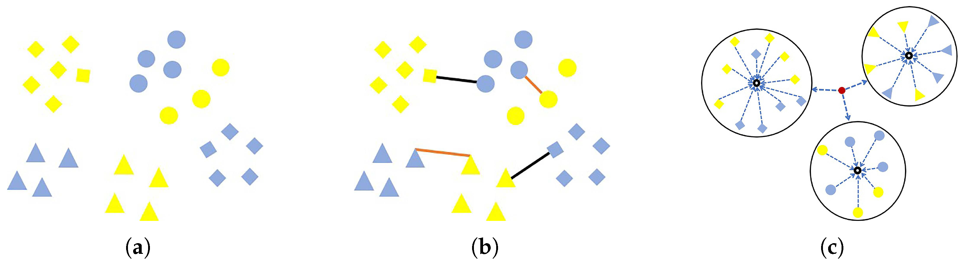
In this paper, we propose a novel representation framework called Transfer of Local Features (TLF) and a novel distance metric called Discriminative Metric Learning (DML). The TLF is a robust representation framework that can adapt to domain variation. It can integrate different kinds of local features, e.g., LBP, LTP and CLBP. The TLF mines the maximum response in regions to make a stable representation for domain variation. By max pooling across different image regions, the pooled feature is salient and more robust to local transformations. We utilize max pooling for two reasons. First, max pooling was advocated by Riesenhuber and Poggio as a more appropriate pooling mechanism for higher-level visual processing such as object recognition, and the max pooling could successfully achieve invariance to image-plane transformations such as translation and scale by building position and scale tolerant complex (C1) cells units [33,34]. Second, Boureau et al. [35] provided a detailed theoretical analysis to prove why max pooling is suitable for classification tasks. The DML not only utilizes sample pairs to learn the distance metric, but also considers the relationship among cloud classes. Specifically, we force the feature vectors from the same class close to their mean vectors, and meanwhile keep the mean vectors of different classes away from the total mean vector. The key idea of DML is to learn a transformation matrix based on the aforementioned considerations. Here, a sample pair consists of a sample from the source domain (yellow) and a sample from the target domain (blue), as illustrated in Figure 2a. To learn a transformation matrix, the input is labelled pairs including similar pairs (orange lines) and dissimilar pairs (black lines) (see Figure 2b). Meanwhile the relationship among cloud classes with respect to the mean vectors should be considered, as shown in Figure 2c. The output is the learned transformation matrix. The excellent property of DML is that it possesses the characteristic of intra-class compactness and maintains the discrimination among classes. Furthermore, in order to improve the practicability of the proposed method, we replace the original cloud images with the convolutional activation maps which are fed into the framework of TLF, and we have obtained significant improvements.
2. Methods
2.1. Review of Local Features
This section presents three representative local features, i.e., LBP [36], LTP [37], and CLBP [38]. The LBP operator is a gray-scale texture operator that characterizes the spatial structure of a local image texture. The LBP operator converts each pixel into a binary string which can be transformed into a decimal number, by computing the sign of the difference between the values of central pixel and its neighbors:
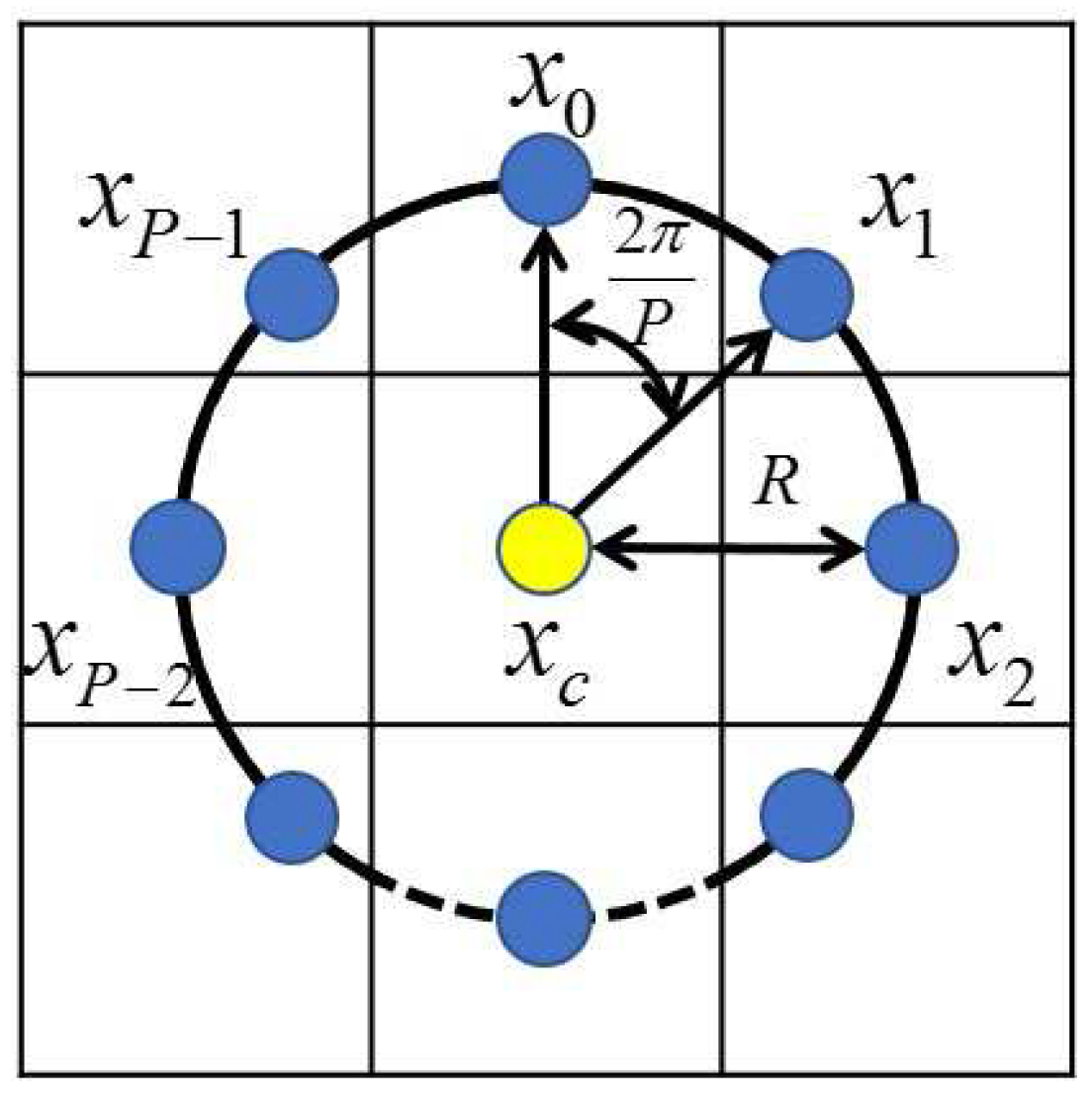
where s is the sign function, is the gray value of the central pixel, is the gray value of the neighbors around the central pixel, and P is the total number of involved neighbors that are evenly distributed in angle on a circle of radius R centered at a pixel. Figure 3a gives an illustration of the LBP method using a structure. The gray values of neighbors that are not in the image grids can be estimated by interpolation, and Figure 4 shows the LBP extraction with .
Since the original LBP is not robust to the image rotation, the rotation invariant LBP operator is proposed, denoted by . It is defined as:
where is a rotation function which performs a circular bitwise right shift k times on the pattern binary string x.
With the number of neighbours surrounding the central pixel increasing, the LBP patterns consequently increase which results in the problem of high dimensionality. For the sake of dimensionality reduction, the uniform LBP operator is proposed and determined by a uniformity measure:
The U value at each pixel reflects the number of spatial transitions between 0 and 1 in the LBP pattern. The uniform LBP patterns are the patterns which satisfy the condition of .
In order to obtain improved rotation invariance and to further reduce the dimensionality, Ojala et al. [36] proposed the rotation invariant uniform LBP operator, denoted by , and it can be expressed as:
where the superscript “riu2” indicates rotation invariant uniform patterns with .
The LTP extends LBP to 3-valued codes by using a threshold . When the gray values between the range of are quantized to zero, ones above are quantized to 1 and ones below to −1. Formally, the 3-valued codes are computed by:
For convenience, each local ternary pattern can be split into positive and negative parts. Each part can be treated as two separate channels of LBP descriptors. Figure 3b gives an illustration of the LTP encoding procedure.
There are three operators in CLBP, including CLBP-Center (CLBP_C), CLBP-Sign (CLBP_S) and CLBP-Magnitude (CLBP_M). Given a central pixel and its P neighbor pixels (t = 0, …, ), the local difference (LD) = – can be decomposed into two components:
where and are the sign and magnitude of , respectively. With Equation (6), [, …, ] is then transformed into a sign vector [, …, ] and a magnitude vector [, …, ]. The sign vector [, …, ] is conducted by the CLBP_S operator which is the same as the original LBP operator. The magnitude vector [, …, ] is conducted by the CLBP_M operator:
where s is the sign function defined in Equation (1), and the threshold is the mean value of from the whole image. In addition, the CLBP_C operator is defined as:
where the threshold is the average gray value of the whole image.
The results of the three operators, i.e., CLBP_C, CLBP_S and CLBP_M, are finally combined to form the CLBP feature. An illustration of the CLBP encoding process is shown in Figure 3c.
2.2. Transfer of Local Features
Figure 1b shows that the conventional LBP, LTP and CLBP are unsuitable for cross-domain ground-based cloud classification, and therefore we propose the TLF to deal with domain shift. The TLF is a region-based feature representation framework. Any kinds of local features integrated to the TLF can be invariant to domain shift, and meanwhile can inherit the properties of integrated local features, such as scale invariance, rotation invariance, and robustness to image noises.
The flowchart of TLF is illustrated in Figure 5, consisting of the following stages:
- (1)
- Image partition stage. We partition a ground-based cloud image into regions with different scales l = 1, 2, 3, as shown in Figure 5b.
- (2)
- Local feature transfer stage. We take the image of regions as an example, and we follow the procedure in the black rectangle of Figure 5c for each region. We first sample local patches in each region using a dense sampling strategy, and then extract local features. Within each patch, we extract histograms of each local feature with three scales , i.e., = (8, 1), (16, 2) and (24, 3). After each patch is represented as a histogram, we apply max pooling strategy on all local histograms for each region, i.e., reserving the maximum response of each histogram bin among all histograms.
- (3)
- Local feature representation stage. The histograms of all regions are concatenated to form a vector representation for each ground-based cloud image, as illustrated in Figure 5d.
There are several excellent properties of the proposed TLF. First, the partition strategy provides multi-scaled local information of a cloud image, which makes the extracted local feature robust to scale changes. Second, employing a dense manner in patch extraction ensure that we can extract information-completed features from local regions. Third, we use max pooling in each region, and the pooled feature achieves some invariance to domain shift, and at the same time captures local region characteristics of a cloud image. Finally, the TLF can integrate various kinds of local features, e.g., LBP, LTP and CLBP. Since in this paper we apply the three local features into the framework of TLF, respectively, we define the three transferred local features as TLBP, TLTP and TCLBP.
2.3. Discriminative Metric Learning
In this section, we describe the proposed DML method in detail. Generally, cloud images from different domains vary in capturing location, occlusion, illumination, resolution and so on. Moreover, while the source domain possesses many labelled cloud images, the target domain has much fewer cloud images. Because of this, it is hardly possible to train a strongly generalized classifier with a few labelled cloud images when we recognize the cloud images from the target domain. Hence, we expect to train a classifier for the target domain with many labelled cloud images from the source domain and few labelled cloud images from the target domain.
There are two feature vectors of cloud images, and , from the source domain and the target domain, respectively. We define the two feature vectors of cloud images as a cross-domain pair . Cross-domain pairs consist of two kinds, similar pairs (a and b belong to the same class) and dissimilar pairs (a and b belong to different classes). Suppose there are N cloud classes in each domain, we construct a set of similar pairs:
and we formulate a set of dissimilar pairs as:
Since the traditional distance metrics, such as Euclidean distance, chi-square metric and Quadratic-Chi (QC) metric are pre-defined and can not adapt to the various sample distributions, we intend to learn a Mahanalobis distance metric to compute the distance between the cross-domain pairs. Specifically, we learn a transformation matrix () and the Mahalanobis distance between a cross-domain pair is defined as:
where is a positive semidefinite matrix.
Our goal is to learn a transformation matrix W in the form of supervision, i.e., all training cloud images are labelled. Many approaches [28,39,40] define a cost function that attempts to maximize the squared distance between dissimilar pairs, while minimize the squared distance between similar pairs. The objective function is formulated as:
where and are the number of dissimilar pairs and similar pairs, respectively. The first constraint is that H is a positive semidefinite matrix which ensures a valid metric, and the second constraint excludes the trivial solution where all distances are zero [40].
The major problem in Equation (12) is that it only considers the relationship between sample pairs, and ignores the relationship among cloud classes which has the high level semantic information. Hence, we expect the feature vectors after transformation have the following two properties. First, the feature vectors from the same class are close to their mean vectors. Second, the mean vectors of different classes are away from the total mean vector, as shown in Figure 2c. Formally, they are formulated as:
where is the mean feature vector of the n-th class, is the the mean feature vector of all training samples, e is the feature vector of a cloud image which can be from both domains, and are constant coefficients, and is the number of feature vectors in the n-th class. The first term maximizes the distance between the different class mean vectors and the total mean vector, which improves the discrimination among classes. The second term results in a high penalty if the feature vectors are far from their mean vector in the transformed feature space, and therefore it can maintain the characteristic of intra-class compactness. Note that can be reformulated as:
and can be transformed in the same way.
In order to learn a discriminative metric learning, we propose to consider sample pairs and the relationship among classes in the learning process, simultaneously. Thus, the objective function of the proposed DML is:
Since the squared Mahalanobis distance between a pair is a scalar, we rewrite the right terms of Equation (11) as:
Similarly, and can be transformed in the same way.
We aim to learn W by maximizing the objective subject to two constraints in Equation (17). is a positive semidefinite matrix, so we can relax the first constraint when explicitly solve for W [28]. We utilize the standard Lagrange multiplier on Equation (17):
Then we take the partial derivative of Equation (18) with the Lagrangian function with respect to W, and set the result equal to zero:
where
This is a standard eigenvector problem. We preserve m eigenvectors of corresponding to the first m largest eigenvalues, and W is equal to:
where is the learned transformation matrix. is the eigenvector of corresponding to the largest eigenvalue, and is the eigenvector of corresponding to the second largest eigenvalue, and so on.
2.4. Convolutional Activations Based Method for Cross-Domain Ground-Based Cloud Classification
Many approaches which utilize convolutional activation maps to obtain image representations have achieved remarkable performance in image processing and computer vision fields [41,42,43]. In the convolutional layer, the filter traverses the input image in the sliding-window manner to generate a convolutional map, which involves the responses of the activations. Hence, we propose to train the CNNs by fine-tuning the VGG-19 model [44] on our cloud databases, and then we extract local features on the convolutional activation maps. Finally, we apply the DML and the nearest neighborhood classifier to recognize the cloud images, as illustrated in Figure 6. Specifically, we add all the convolutional activation maps of one convolutional layer to capture the completed spatial response information of clouds. Let denote the convolutional summing map (CSM) and it is formulated as:
where denotes the activation response of the k-th convolutional activation map and K is the number of the convolutional activation maps.
3. Results and Discussion
In this section, we first introduce the databases and experimental setup. It is should be noted that the cloud images are captured by an RGB color camera. Second, we verify the effect of TLF, DML and CSM on three databases, i.e., the CAMS database, the IAP database and the MOC database. Then, we compare the proposed method with other excellent methods. Finally, in order to better understand the proposed method, we analyze it in three aspects: the role of max pooling, the influence of projected feature space dimensions, and the role of the fraction of cloud images from the target domain.
3.1. Databases and Experimental Setup
The first cloud database is the CAMS database, which is provided by Chinese Academy of Meteorological Sciences. According to the international cloud classification system published in World Meteorological Organization (WMO), the database is divided into seven classes. Note that the class of clear sky includes not only images without clouds but also images with cloudiness below 10%. The sample numbers in each class are different and the total number is 1600 as listed in Table 1. The cloud images in this database are captured in Yangjiang, Guangdong Province, China, and have pixels. The cloud images have a weak illumination and no occlusion. The sundisk is considered as a virtual cloud for the CAMS database. Samples for each class are shown in Figure 7a.
The second cloud database is the IAP database, which is provided by Institute of Atmospheric Physics, Chinese Academy of Sciences. The database is also divided into seven classes. The sample number of each class is different and the total number is 1518 as listed in Table 1. The cloud images in this database are captured in the same location as the CAMS database, but the acquisition device is different from that of the CAMS database. The cloud images from the IAP database have pixels, a strong illumination and occlusion. Note that the occlusion in cloud images is caused by a part of the camera. Samples for each class are shown in Figure 7b.
The third cloud database is the MOC database, which is provided by Meteorological Observation Centre, China Meteorological Administration. The database is divided into seven class as well. The total sample number is 1397 and the detail sample number for each class is listed in Table 1. Different from the first two cloud databases, the cloud images in this database are taken in Wuxi, Jiangsu Province, China. Moreover, the cloud images have pixels with a strong illumination and occlusion. Samples for each class are shown in Figure 7c.
It is obvious that cloud images from the three cloud databases vary in location, illumination, occlusion and resolution. Hence, the cloud images distribute in three different domains and the differences are listed in Table 2.
All images from the three databases were scaled to pixels and then the intensity of each cloud image was normalized to an average intensity of 128 with a standard deviation of 20. This normalization reduced the effects of illumination variance across images. Finally, we adjusted the geometry of the cloud images to uniform representation, and the sample image is shown in Figure 8. Furthermore, we adopted the feature normalization (FN) step for image representation. Specifically, as for the LBP, LTP and CLBP, the feature vectors were normalized to zero-mean unit-variance vectors, and then were concatenated. As for the TLBP, TLTP and TCLBP, the feature vector of each region was normalized to a zero-mean unit-variance vector, and then was concatenated. We selected all cloud images from the source domain and a half of cloud images in each class from the target domain at random as training images, and the remaining of the target domain as test images. This procedure was independently implemented 10 times and the final results represented the average accuracy over these 10 random splits. We implemented our algorithm on a desktop PC with an Intel Xeon CPU E5-2660 v2 @2.20GHz and 64 Gbytes memory in Matlab 2013b. LBP requires 35.2 s for each cloud image, while TCLBP requires 56.8 s for each cloud image.
The nearest neighborhood classifier was used to classify the cloud images. The metrics employed to evaluate the goodness-of-fit between two histograms included predefined metrics, metric learning (ML) and the proposed distance metric (DML). Note that the key idea of metric learning is to project the original inputs into another feature space, and then calculate Euclidean distance in the projected feature space. Hence, as for the selection of predefined metrics, we chose Euclidean distance metric (Euclid) as the similarity measurement in the following contrasting experiments.
3.2. Effect of TLF
We compared the TLBP, TLTP and TCLBP with the LBP, LTP and CLBP, respectively. Specifically, we extracted LBP feature with equal to (8, 1), (16, 2) and (24, 3), and then concatenated histograms of the three scales to form a feature vector for each cloud image. So the final feature vector of each cloud image has 10 + 18 + 26 = 54 dimensions. The LTP can be divided into two LBPs, positive LBP and negative LBP. Then two histograms are concatenated into one histogram, so a cloud image is finally represented as a = 108 dimensional feature vector. For the CLBP, the three operators, CLBP_C, CLBP_S and CLBP_M, can be combined hybridly. Specifically, a 2D joint histogram, “CLBP_S/C” is built first, and then the histogram is converted to a 1D histogram, which is then concatenated with CLBP_M to generate a joint histogram. The dimension is () + () + () = 162. When applied the three features to the TLF, the dimension of TLBP is + + = 756, and likewise, the dimensions of TLTP and TCLBP are 1512 and 2268, respectively.
The experimental results are listed in Table 3. The first numbers in the bracket show the basic results. The remaining two numbers in the bracket show the results with image geometric correction (IGC), and with both IGC and feature normalization (FN), respectively. From the basic results, it can be seen that the proposed TLBP, TLTP and TCLBP achieve higher accuracies than LBP, LTP and CLBP, respectively, and the TCLBP achieves the best performance in all 6 situations. That’s because TLBP, TLTP and TCLBP are extracted by dense sampling which could obtain more stable and completed cloud information in local regions. We further apply max pooling on all local features for each region to obtain features which are more robust to local transformations. Hence, applying the TLF to the local features is a good choice to adapt to domain shift. Furthermore, when we take the MOC database as the source domain, and the CAMS database as the target domain, we obtain the poorest performance compared with other combinations of the source and target domains. The reason is that the MOC database is greatly different from the CAMS database in illumination, capturing location, occlusion and image resolution. With the help of IGC, the accuracies improve by about 4%. Based on IGC and FN, the accuracies further improve by about 3%.
3.3. Effect of DML
We compared the proposed DML with Euclidean distance metric (Euclid) and ML to classify cloud images with the six kinds of features. The experimental results are listed in Table 4 and Table 5. The first numbers in the bracket show the basic results. The remaining two numbers in the bracket show the results with IGC, and with both IGC and FN, respectively. From the basic results, several conclusions can be drawn. First, the performance improves with the help of ML. It is because ML is a data-driven method which learns the intrinsic topology structure between the source and target domains. This indicates that ML is fitter for evaluating the similarity between the sample pairs. Second, as for traditional and transferred features, the classification accuracies increase significantly with DML, all increased by over 3% comparing to ML. It demonstrates that the consideration of the relationship among cloud classes in the learning process of DML can boost the performance. Third, the transferred features perform better than the traditional ones, which further proves the effectiveness of the proposed TLF both in pre-defined metric and learning-based metric. Particularly, the combination of TCLBP and DML outperforms the other compared methods in all situations. The case of MOC to CAMS domain shift still achieves the lowest classification accuracy in all situations. For example, comparing to TCLBP + Euclid and TCLBP + ML, the performance of TCLBP + ML rises by 2.85% and 4.35%, respectively. While other cases of domain shift, the improvements of classification accuracies are lower than the case of MOC to CAMS domain shift. It is further verified that DML can solve the classification issue that two domains are greatly different. With the help of IGC, the accuracies improve by about 4%. Based on IGC and FN, the accuracies further improve by about 3%.
In order to further analyse the effectiveness of the proposed method TCLBP + DML (without IGC and FN), we utilized the confusion matrix to show the detailed performance of each category in the case of IAP to MOC domain shift, as shown in Figure 9. The element of row i and column j in confusion matrix means the percentage of the i-th cloud class being recognized as the j-th cloud class. The proposed method can achieve the best performance in classifying ‘Clear sky’. ‘Cirrocumulus and altocumulus’ is likely to incorrectly be discriminated as ‘Cirrus and cirrostratus’, and ‘Cumulonimbus and nimbostratus’ is likely to incorrectly be discriminated as ‘Stratocumulus’. The incorrect discrimination of ‘Cumulus’ as ‘Clear sky’ is relatively high, and the reason is as follows. Some images of ‘Cumulus’ in the IAP database contain a few of ‘Cumulus’ clouds which are with cloudiness more than 10% (such as 15%). While some images of ‘Clear sky’ in the MOC database include not only images without clouds but also images with cloudiness below 10%. Hence, some images of the two classes are similar and easily misclassified.
3.4. Effect of CSM
In this section, we conducted the experiments based on the cloud images after IGC and FN. First, we concatenated the TLBP, TLTP and TCLBP to form a feature vector for a cloud image, and Table 6 shows the classification accuracies with different metrics. Comparing to TCLBP + DML, the classification accuracies increase by over 7% in all situations. Second, we took the fixed-size RGB cloud images that the red, green and blue bands were all used as the input to the CNNs, and employed the convolutional activation maps of the eighth convolutional layer with 256 kernels of size . Then, we concatenated the TLBP, TLTP and TCLBP with CSM. The experimental results are shown in Table 7. With the help of CSM, the classification accuracies all further increase by about 15%.
3.5. Comparison to the State-Of-The-Art Methods
We compared the performance of the proposed method TCLBP + DML with two state-of-the-art methods, bag of words (BoW) [45] and multiple random projections (MRP) [46]. For the BoW method, we first extracted patch features for each cloud image. Each patch feature was an 81 dimensional vector, which was formed by stretching a neighborhood around each pixel. All the patch vectors were normalized using Weber’s law [47]. Then, we utilized K-means clustering [48] over patch vectors to learn a dictionary. The size of dictionary for each class was set to be 300, which resulted in a 2100 dimensional vector for each cloud image. Finally, feature vectors of all cloud images were fed into a support vector machine (SVM) classifier with the radial basis function (RBF) kernel for classification. The MRP is a patch-based method. We selected the patch size of , and followed the procedure in [46]. For fair comparison, we followed the same experimental setting as mentioned in Section 3.1 for the three methods.
The experimental results are listed in Table 8. The sixth column shows the results of TCLBP + DML with IGC, and the seventh column shows the results of TCLBP + DML with IGC and FN. It is obvious that BoW and MRP do not adapt to cross-domain ground-based cloud classification. The BoW and MRP are learning-based method which encodes cloud images by using the learned dictionary, but they take raw pixel intensities as features which are not robust to local transformations. In contrast, we utilize a stable feature representation to solve the problem of domain shift, and take sample pairs and the relationship among cloud classes into consideration to learn a discriminative metric.
3.6. Discussion of the Proposed Method
We analyzed the proposed method in three aspects with the basic results, including the role of max pooling, the influence of projected feature space dimensions, and the role of the fraction of cloud images from the target domain. Note that we took the CLBP and TCLBP as examples.
3.6.1. Role of Max Pooling
The cross-domain ground-based cloud classification is largely affected by changes in image resolution, illumination and occlusion, which should be addressed in feature representation and similarity measurement. The application of max pooling in TLF is an effective strategy to overcome changes in illumination, image resolution or occlusion. For fair comparison, we partitioned a cloud image into regions with different scales l = 1, 2, 3, and utilized a subwindow with the size of to densely sample the local patches with an overlap step of 5 pixels. We extracted CLBP feature in each patch, and then aggregated all features in each region using average pooling which preserved the average response of each histogram bin among all histograms. Each cloud image was also represented as a 2268-dimensional feature vector. We defined the feature as multi-CLBP. By comparing the multi-CLBP without max pooling and TCLBP in different metrics, we found that this operation does improve the performance of cross-domain ground-based cloud classification, as illustrated in Figure 10. With max pooling, the classification results are improved by about 5% in all situations with different metrics.
3.6.2. Influence of Parameter Variances
For the proposed DML, the dimensions of the projected space has an influence on performance. In other words, the parameter m in Equation (24) controls the dimension of W and as a result affects classification accuracies. This influence is shown in Figure 11, obtained by experiments on the IAP to MOC domain shift. Approximately, the performance is increasing with dimension increasing, but it decreases after 200 dimensions. The best experimental result is obtained with m equal to 200.
3.6.3. Role of the Fraction of Cloud Images from the Target Domain
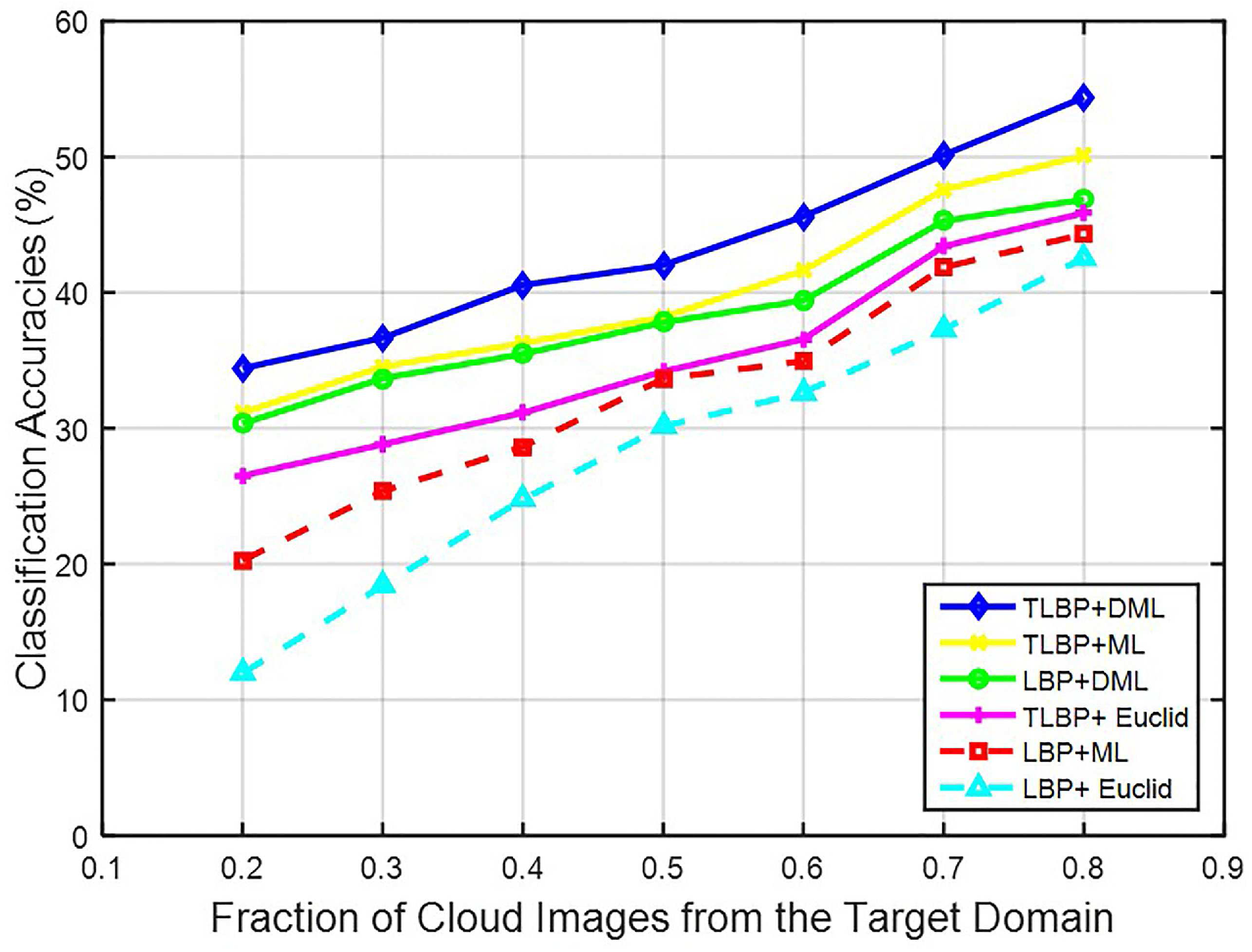
We varied the fraction of cloud images in each class from the target domain in increment of 20% up to 80%. The training images consisted of two parts, all cloud images from the source domain, and a fraction of cloud images from the target domain. We took the MOC to CAMS domain shift as an example. The average recognition accuracies for different fractions are shown in Figure 12. The classification capabilities of various methods reduce significantly when the number of cloud images from the target domain decreases. In contrast, our method outperforms other approaches with a tolerable accuracy due to adopting the stable feature representation and discriminative metric.
4. Conclusions
In this paper, we have presented an effective method for cross-domain ground-based cloud classification. We have proposed a novel local feature representation called TLF, which is shown to be robust against domain shift, such as changes in illumination, image resolution, capturing location, and occlusion. In addition, we have proposed a novel metric learning named DML. There are the high level semantic information among cloud classes, so we consider the relationship among them in the learning process of DML. We have conducted a series of experiments to verify the proposed method on three cloud databases, the CAMS, MOC and IAP. By Comparing to the state-of-the-art methods, the experimental results demonstrate the proposed method achieves the best performance. Furthermore, in order to improve the practicability of the proposed method, we replace the original cloud images with CSM. Then, we apply CSM to TLF and DML, and we have obtained significant improvements.
Acknowledgments
This work was supported by National Natural Science Foundation of China under Grant No. 61501327, No. 61711530240 and No. 61401309, Natural Science Foundation of Tianjin under Grant No. 17JCZDJC30600, and No. 15JCQNJC01700, the Fund of Tianjin Normal University under Grant No.135202RC1703, and the Open Projects Program of National Laboratory of Pattern Recognition under Grant No. 201700001.
Author Contributions
All authors made significant contributions to the manuscript. Zhong Zhang and Donghong Li conceived, designed and performed the experiments, and wrote the paper; Shuang Liu performed the experiments and analyzed the data; Baihua Xiao and Xiaozhong Cao provided the background knowledge of cloud classification, reviewed the paper and gave constructive advices.
Conflicts of Interest
The authors declare no conflict of interest.
References
- Cui, F.; Ju, R.; Ding, Y.; Ding, H.; Cheng, X. Prediction of regional global horizontal irradiance combining ground-based cloud observation and numerical weather prediction. Adv. Mat. Res. 2014, 1073, 388–394. [Google Scholar] [CrossRef]
- Várnai, T.; Marshak, A. Effect of cloud fraction on near-cloud aerosol behavior in the MODIS atmospheric correction ocean color product. Remote Sens. 2015, 7, 5283–5299. [Google Scholar] [CrossRef]
- Ebert, E.E. Pattern recognition analysis of polar clouds during summer and winter. Int. J. Remote Sens. 1992, 13, 97–109. [Google Scholar] [CrossRef]
- Musial, J.P.; Hüsler, F.; Sütterlin, M.; Neuhaus, C.; Wunderle, S. Probabilistic approach to cloud and snow detection on advanced very high resolution radiometer (AVHRR) imagery. Atmos. Meas. Tech. 2014, 7, 799–822. [Google Scholar] [CrossRef] [Green Version]
- Lamei, N.; Hutchison, K.D.; Crawford, M.M.; Khazenie, N. Cloud-type discrimination via multispectral textural analysis. Opt. Eng. 1994, 33, 1303–1313. [Google Scholar]
- Costa, M.J.; Bortoli, D. Cloud detection and classification from multi-spectral satellite data. In Proceedings of the International Society for Optical Engineering, Remote Sensing of Clouds and the Atmosphere XIV, Berlin, Germany, 31 August–1 September 2009; Volume 7475. [Google Scholar]
- Lee, K.-Y.; Lin, C.-H. Cloud detection of optical satellite images using support vector machine. In Proceedings of the International Archives of the Photogrammetry, Remote Sensing and Spatial Information Sciences, Prague, Czech Republic, 12–19 July 2016; pp. 289–293. [Google Scholar]
- Yool, S.R.; Brandley, M.; Kern, C.; Gerlach, F.W.; Rhodes, K.L. Remote discrimination of clouds using a neural network. In Proceedings of the Neural and Stochastic Methods in Image and Signal Processing, San Diego, CA, USA, 20–23 July 1992; pp. 497–504. [Google Scholar]
- Lee, J.; Weger, R.C.; Sengupta, S.K.; Welch, R.M. A neural network approach to cloud classification. IEEE Trans. Geosci. Remote Sens. 1990, 28, 846–855. [Google Scholar] [CrossRef]
- Taravat, A.; Frate, F.D.; Cornaro, C.; Vergari, S. Neural networks and support vector machine algorithms for automatic cloud classification of whole-sky ground-based images. IEEE Trans. Geosci. Remote Sens. 2015, 12, 666–670. [Google Scholar] [CrossRef]
- Shields, J.E.; Karr, M.E.; Tooman, T.P.; Sowle, D.H.; Moore, S.T. The whole sky imager—A year of progress. In Proceedings of the Eighth Atmospheric Radiation Measurement Science Team Meeting, Tucson, AZ, USA, 23–27 March 1998; pp. 23–27. [Google Scholar]
- Cazorla, A.; Olmo, F.J.; Alados-Arboledas, L. Development of a sky imager for cloud cover assessment. J. Opt. Soc. Am. A 2008, 25, 29–39. [Google Scholar] [CrossRef]
- Shaw, J.A.; Thurairajah, B.; Edqvist, E.; Mizutan, K. Infrared cloud imager deployment at the north slope of Alaska during early 2002. In Proceedings of the Twelfth Atmospheric Radiation Measurement Science Team Meeting, St. Petersburg, FL, USA, 8–12 April 2002; pp. 1–7. [Google Scholar]
- Sun, X.J.; Gao, T.C.; Zhai, D.L.; Zhao, S.J.; Lian, J.G. Whole sky infrared cloud measuring system based on the uncooled infrared focal plane array. Infrared Laser Eng. 2008, 37, 761–764. [Google Scholar]
- Singh, M.; Glennen, M. Automated ground-based cloud recognition. Pattern Anal. Appl. 2005, 8, 258–271. [Google Scholar] [CrossRef]
- Calbo, J.; Sabburg, J. Feature extraction from whole-sky ground-based images for cloud-type recognition. J. Atmos. Ocean Technol. 2008, 25, 3–14. [Google Scholar] [CrossRef]
- Heinle, A.; Macke, A.; Srivastav, A. Automatic cloud classification of whole sky images. Atmos. Meas. Tech. 2010, 3, 557–567. [Google Scholar] [CrossRef] [Green Version]
- Kazantzidis, A.; Tzoumanikas, P.; Bais, A.F.; Fotopoulos, S.; Economou, G. Cloud detection and classification with the use of whole-sky ground-based images. Atmos. Res. 2012, 113, 80–88. [Google Scholar] [CrossRef]
- Pentland, A.P. Fractal-based description of natural scenes. IEEE Trans. Pattern Anal. Mach. Intell. 1984, 6, 661–674. [Google Scholar] [CrossRef] [PubMed]
- Isosalo, A.; Turtinen, M.; Pietikäinen, M. Cloud characterization using local texture information. In Proceedings of the Finnish Signal Processing Symposium, Oulu, Finland, 30 August 2007; pp. 1–6. [Google Scholar]
- Xiao, Y.; Cao, Z.; Zhuo, W.; Ye, L.; Zhu, L. mCLOUD: A multiview visual feature extraction mechanism for ground-based cloud image categorization. J. Atmos. Ocean. Technol. 2016, 33, 789–801. [Google Scholar] [CrossRef]
- Liu, S.; Wang, C.; Xiao, B.; Zhang, Z.; Shao, Y. Salient local binary pattern for ground-based cloud classification. Acta Meteorol. Sin. 2013, 27, 211–220. [Google Scholar] [CrossRef]
- Liu, S.; Wang, C.; Xiao, B.; Zhang, Z.; Shao, Y. Illumination-invariant completed LTP descriptor for cloud classification. In Proceedings of the 5th International Congress on Image and Signal Processing, Chongqing, China, 16–18 October 2012; pp. 449–453. [Google Scholar]
- Huertas-Tato, J.; Rodríguez-Benítez, F.J.; Arbizu-Barrena, C.; Aler-Mur, R.; Galvan-Leon, I.; Pozo-Vázquez, D. Automatic cloud-type classification based on the combined use of a sky camera and a ceilometer. J. Geophys. Res. Atmos. 2017, 122, 11045–11061. [Google Scholar] [CrossRef]
- Wang, L.; Zhang, Y.; Feng, J. On the Euclidean distance of images. IEEE Trans. Pattern Anal. Mach. Intell. 2005, 27, 1334–1339. [Google Scholar] [CrossRef] [PubMed]
- Xing, E.P.; Jordan, M.I.; Russell, S.J.; Ng, A.Y. Distance metric learning with application to clustering with side-information. In Proceedings of the 16th Annual Conference on Neural Information Processing Systems, Vancouver/Whistler, BC, Canada, 8–13 December 2003; pp. 521–528. [Google Scholar]
- Weinberger, K.Q.; Blitzer, J.; Saul, L.K. Distance metric learning for large margin nearest neighbor classification. J. Mach. Learn. Res. 2009, 10, 207–244. [Google Scholar]
- Alipanahi, B.; Biggs, M.; Ghodsi, A. Distance metric learning vs. Fisher discriminant analysis. In Proceedings of the 23rd National Conference on Artificial Intelligence, Chicago, IL, USA, 13–17 July 2008; pp. 598–603. [Google Scholar]
- Zhao, C.; Wang, X.; Wong, W.K.; Zheng, W.; Yang, J.; Miao, D. Multiple metric learning based on bar-shape descriptor for person re-identification. Pattern Recognit. 2017, 71, 218–234. [Google Scholar] [CrossRef]
- Saenko, K.; Kulis, B.; Fritz, M.; Darrell, T. Adapting visual category models to new domains. In Proceedings of the European Conference on Computer Vision, Heraklion, Crete, Greece, 5–11 September 2010; pp. 213–226. [Google Scholar]
- Ding, Z.; Fu, Y. Robust transfer metric learning for image classification. IEEE Trans. Image Process. 2017, 26, 660–670. [Google Scholar] [CrossRef] [PubMed]
- Yang, C.; Tan, Y.; Bruzzone, L.; Lu, L.; Guan, R. Discriminative feature metric learning in the affinity propagation model for band selection in hyperspectral images. Remote Sens. 2017, 9, 782. [Google Scholar] [CrossRef]
- Riesenhuber, M.; Poggio, T. Hierarchical models of object recognition in cortex. Nat. Neurosci. 1999, 2, 1019–1025. [Google Scholar] [CrossRef] [PubMed]
- Serre, T.; Wolf, L.; Poggio, T. Object recognition with features inspired by visual cortex. In Proceedings of the IEEE Computer Society Conference on Computer Vision and Pattern Recognition, San Diego, CA, USA, 20–26 June 2005; pp. 994–1000. [Google Scholar]
- Boureau, Y.L.; Ponce, J.; LeCun, Y. A theoretical analysis of feature pooling in visual recognition. In Proceedings of the 27th International Conference on Machine Learning, Haifa, Israel, 21–25 June 2010; pp. 111–118. [Google Scholar]
- Ojala, T.; Pietikainen, M.; Maenpaa, T. Multiresolution gray-scale and rotation invariant texture classification with local binary patterns. IEEE Trans. Pattern Anal. Mach. Intell. 2002, 24, 971–987. [Google Scholar] [CrossRef]
- Tan, X.; Triggs, B. Enhanced local texture feature sets for face recognition under difficult lighting conditions. IEEE Trans. Image Process. 2010, 19, 1635–1650. [Google Scholar] [PubMed]
- Guo, Z.; Zhang, L.; Zhang, D. A completed modeling of local binary pattern operator for texture classification. IEEE Trans. Image Process. 2010, 19, 1657–1663. [Google Scholar] [PubMed]
- Globerson, A.; Roweis, S. Metric learning by collapsing classes. In Proceedings of the 19th Annual Conference on Neural Information Processing Systems, Vancouver, BC, Canada, 4–7 December 2006; pp. 451–458. [Google Scholar]
- Ghodsi, A.; Wilkinson, D.; Southey, F. Improving embeddings by flexible exploitation of side information. In Proceedings of the 22nd National Conference on Artificial Intelligence, Vancouver, BC, Canada, 22–26 July 2007; pp. 810–816. [Google Scholar]
- Babenko, A.; Lempitsky, V. Aggregating local deep features for image retrieval. In Proceedings of the IEEE International Conference on Computer Vision, Santiago, Chile, 13–16 December 2015; pp. 1269–1277. [Google Scholar]
- Cimpoi, M.; Maji, S.; Vedaldi, A. Deep filter banks for texture recognition and segmentation. In Proceedings of the IEEE Conference on Computer Vision and Pattern Recognition, Boston, MA, USA, 7–12 June 2015; pp. 3828–3836. [Google Scholar]
- Shi, B.; Wang, X.; Lyu, P.; Yao, C.; Bai, X. Robust scene text recognition with automatic rectification. In Proceedings of the IEEE Conference on Computer Vision and Pattern Recognition, Seattle, WA, USA, 27–30 June 2016; pp. 4168–4176. [Google Scholar]
- Simonyan, K.; Zisserman, A. Very deep convolutional networks for large-scale image recognition. arXiv, 2014; arXiv:1409.1556. [Google Scholar]
- Leung, T.; Malik, J. Representing and recognizing the visual appearance of materials using three-dimensional textons. Int. J. Comput. Vis. 2001, 43, 29–44. [Google Scholar] [CrossRef]
- Liu, S.; Wang, C.; Xiao, B.; Zhang, Z.; Shao, Y. Ground-based cloud classification using multiple random projections. In Proceedings of the International Conference on Computer Vision in Remote Sensing, Xiamen, China, 16–18 December 2012; pp. 7–12. [Google Scholar]
- Liu, L.; Fieguth, P. Texture classification from random features. IEEE Trans. Pattern Anal. Mach. Intell. 2012, 34, 574–586. [Google Scholar] [CrossRef] [PubMed]
- Lloyd, S. Least squares quantization in PCM. IEEE Trans. Inf. Theory 1982, 28, 129–137. [Google Scholar] [CrossRef]
Figure 1.
(a) Cloud examples from two different domains. In the source domain, the lower right image: the sun seems to be on the right, while in the target domain image, the sun seems to be on the left; (b) When these samples are trained in the source domain (S) and tested in the target domain (T), the classification accuracies of three representative methods, i.e., LBP, LTP and CLBP, decrease rapidly.
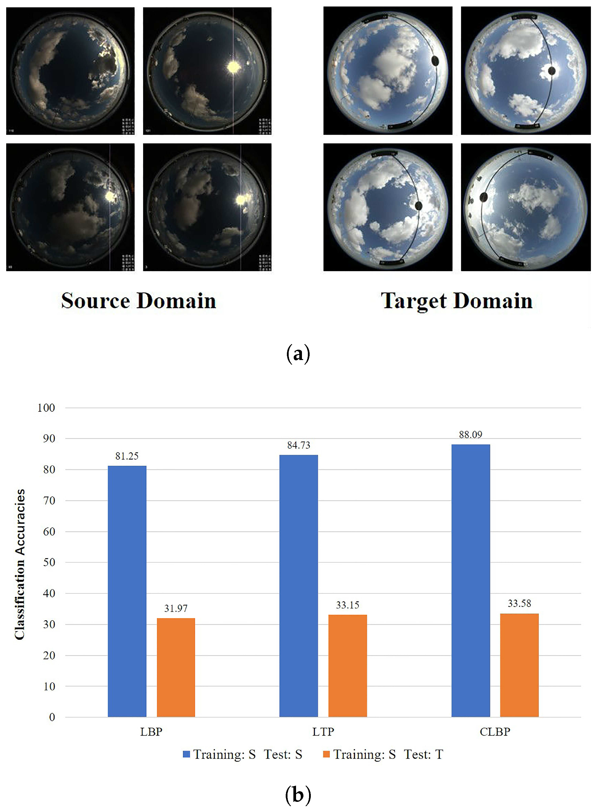
Figure 2.
(a) Two different original domains (yellow and blue); (b) Applying pairwise samples including similar pairs (orange lines) and dissimilar pairs (black lines) constraints to the original domains; (c) Forcing the feature vectors from the same class to their mean vectors (black circular rings), and meanwhile keeping the mean vectors of different classes away from the total mean vector (the red circular).

Figure 3.
The encoding process of (a) LBP, (b) LTP, and (c) CLBP for a structure.

Figure 4.
Central pixel and its P circularly and evenly spaced neighbors with radius R.

Figure 5.
(a) An original cloud image; (b) the original cloud image is divided into regions with different scales l = 1, 2, 3; (c) feature extraction and representation; (d) the final feature representation of the cloud image.
Figure 5.
(a) An original cloud image; (b) the original cloud image is divided into regions with different scales l = 1, 2, 3; (c) feature extraction and representation; (d) the final feature representation of the cloud image.
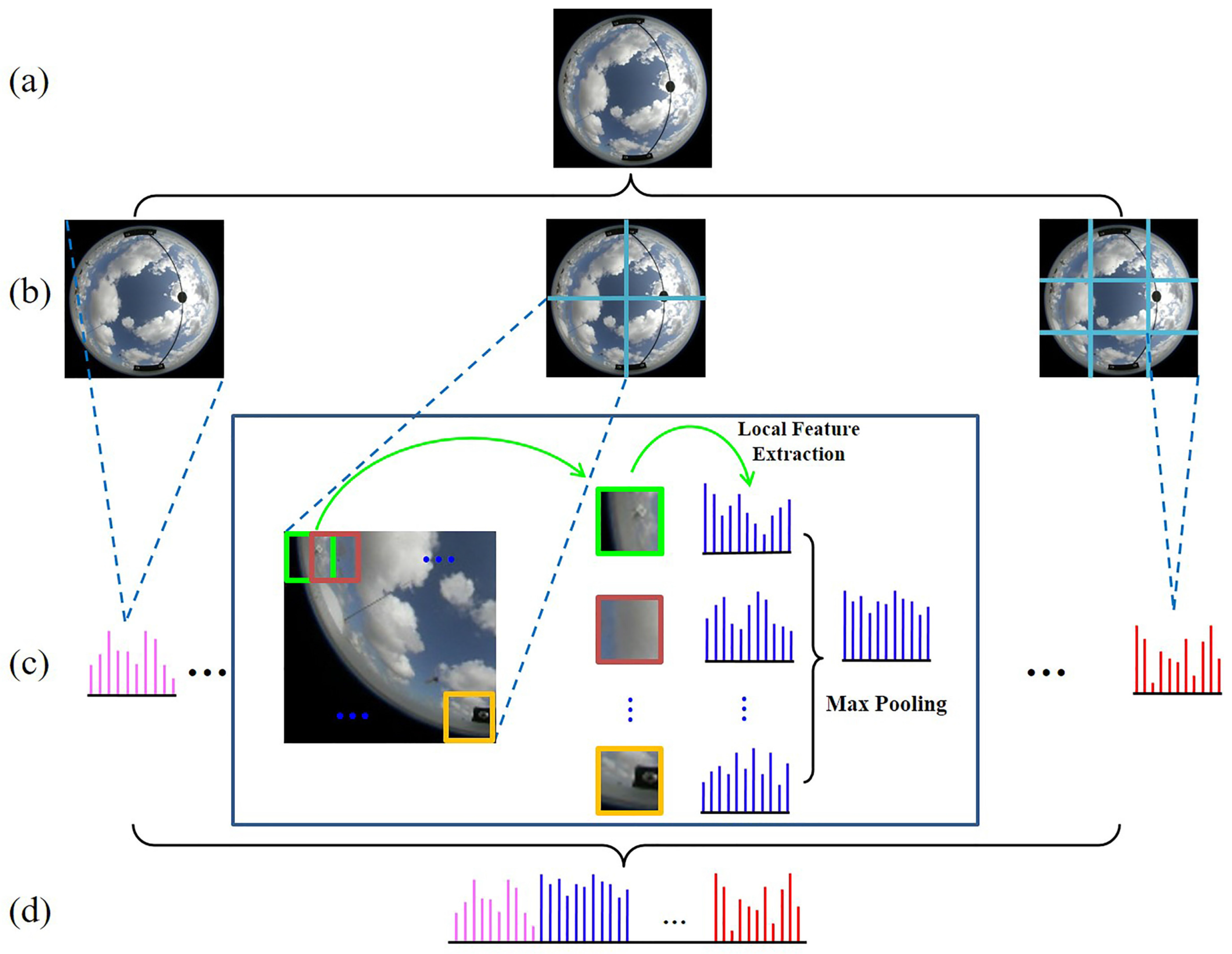
Figure 6.
The architecture of the proposed method based on CNNs for cross-domain ground-based cloud classification.
Figure 6.
The architecture of the proposed method based on CNNs for cross-domain ground-based cloud classification.
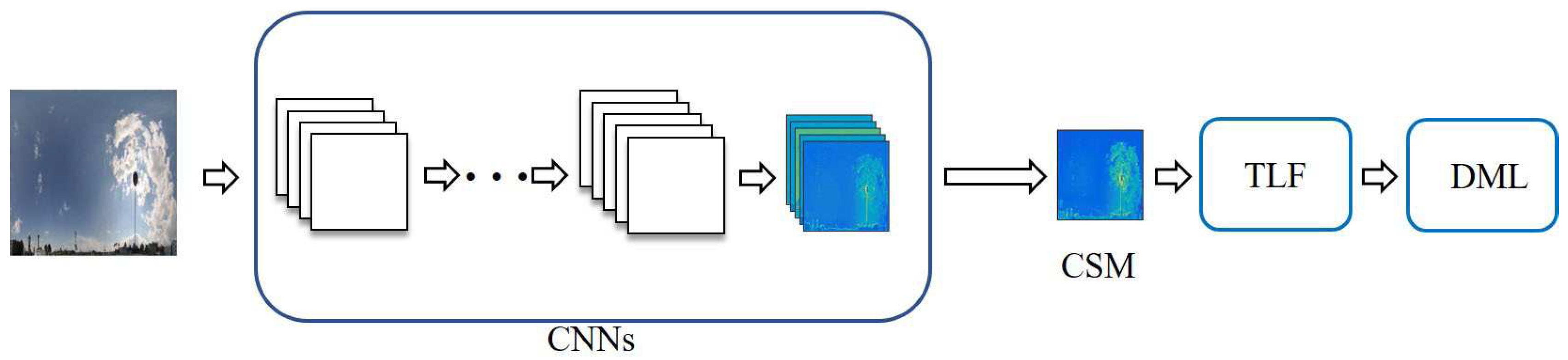
Figure 7.
Cloud samples from (a) the CAMS database, (b) the IAP database, and (c) the MOC database.
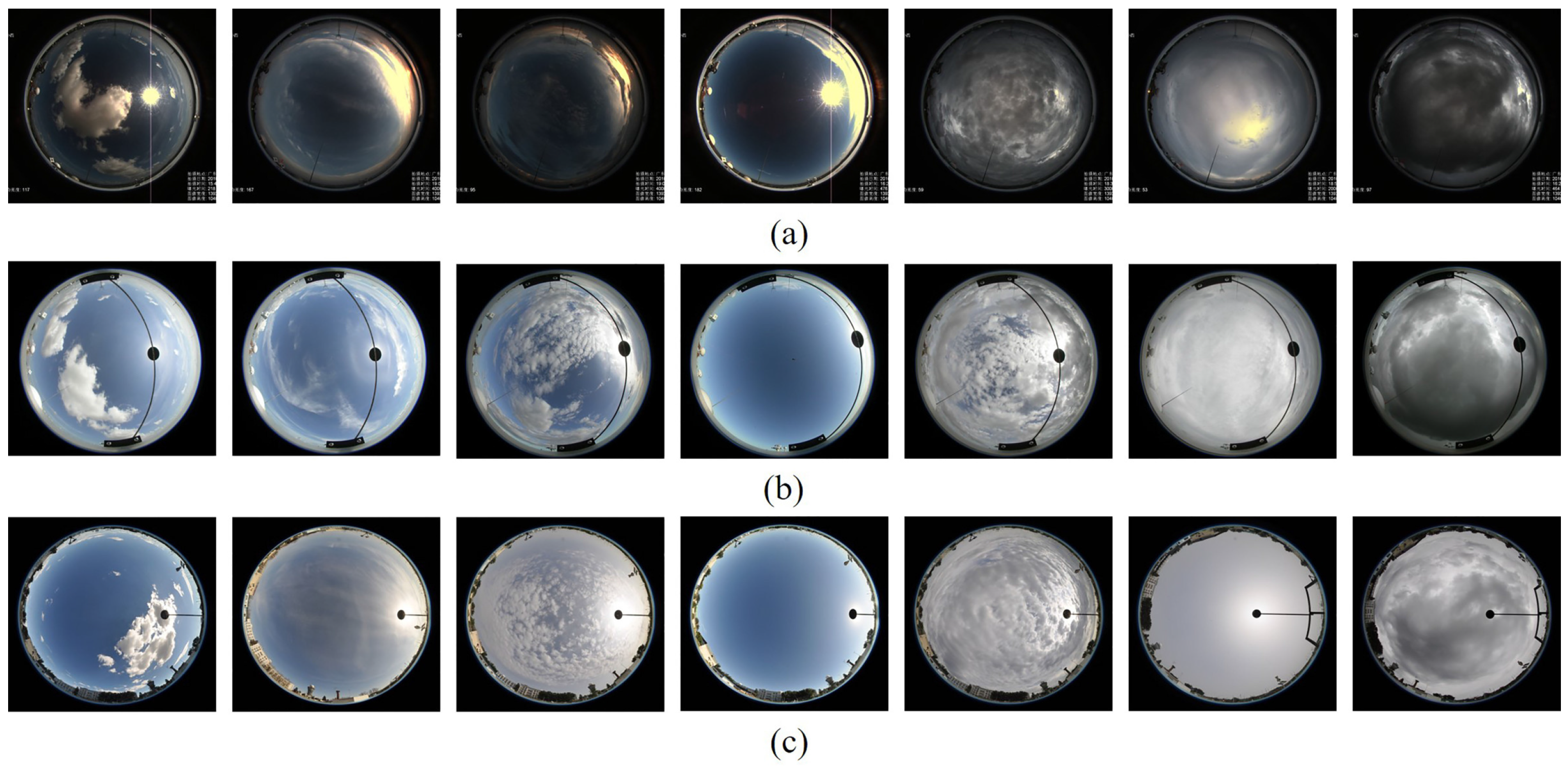
Figure 8.
(a) The original cloud image, and (b) the cloud image after geometric correction.
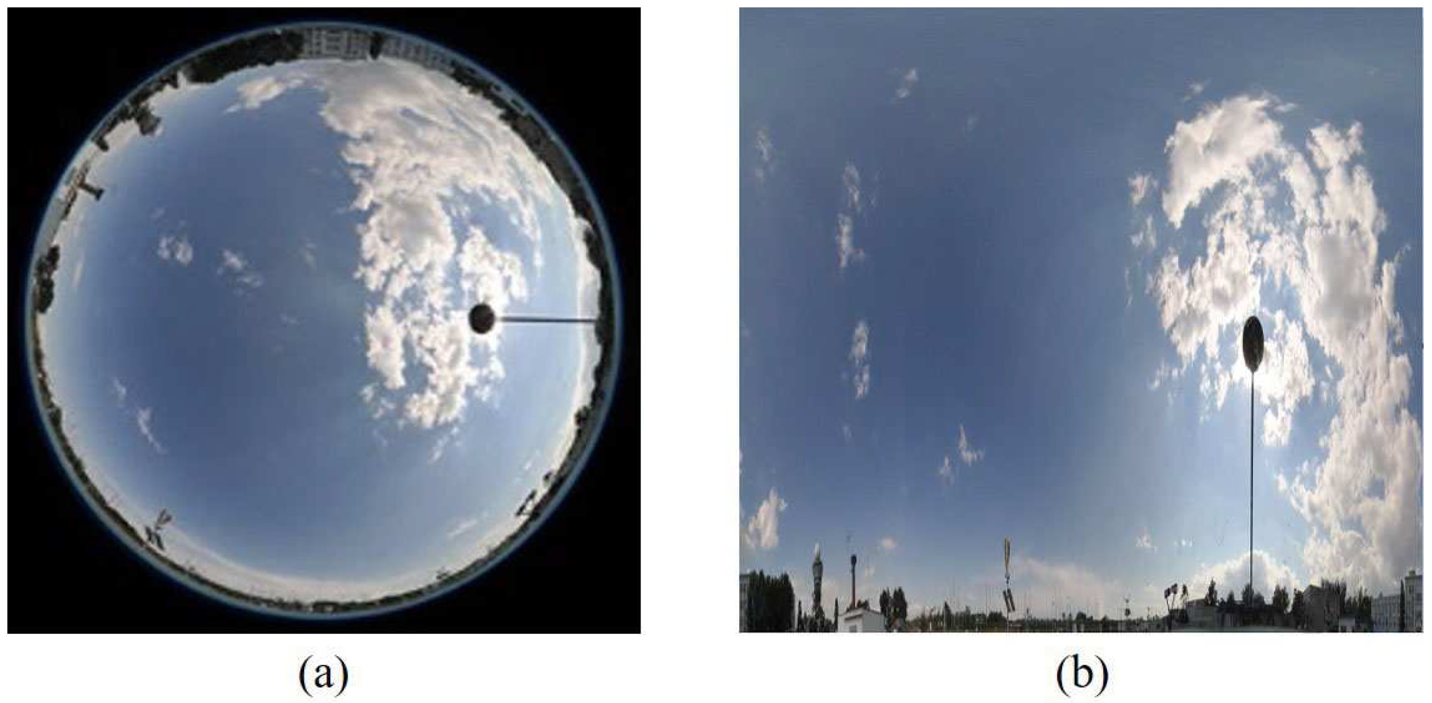
Figure 9.
The confusion matrix for the best case TCLBP + DML (without IGC and FN) in the case of IAP to MOC domain shift. The Arabic numbers denote 1: Cumulus, 2: Cirrus and cirrostratus, 3: Cirrocumulus and altocumulus, 4: Clear sky, 5: Stratocumulus, 6: Stratus and altostratus, 7: Cumulonimbus and nimbostratus, respectively.
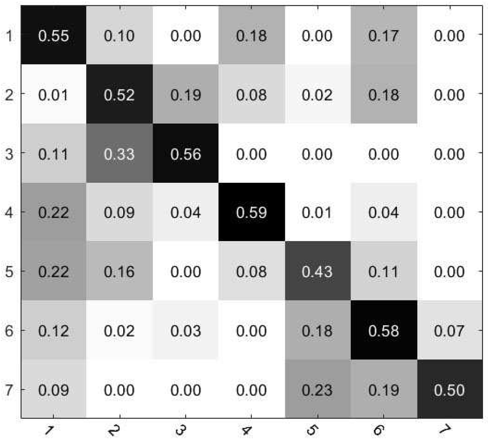
Figure 10.
(a–c) We implement 6 cross-domain classification experiments with different metrics. The Arabic numbers in abscissa denote the domain shifts of CAMS to IAP, CAMS to MOC, IAP to CAMS, IAP to MOC, MOC to CAMS, MOC to IAP, respectively.
Figure 10.
(a–c) We implement 6 cross-domain classification experiments with different metrics. The Arabic numbers in abscissa denote the domain shifts of CAMS to IAP, CAMS to MOC, IAP to CAMS, IAP to MOC, MOC to CAMS, MOC to IAP, respectively.
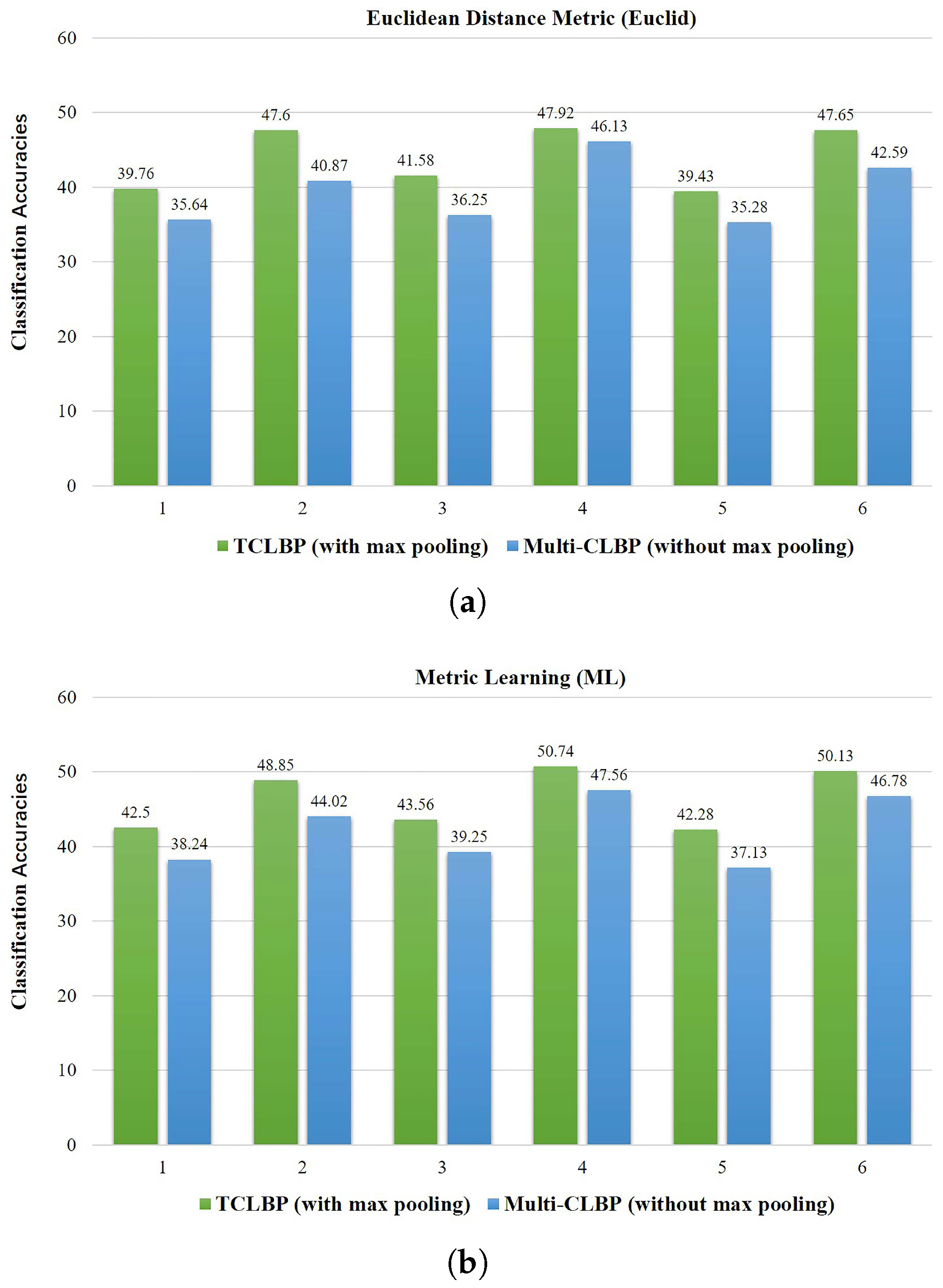
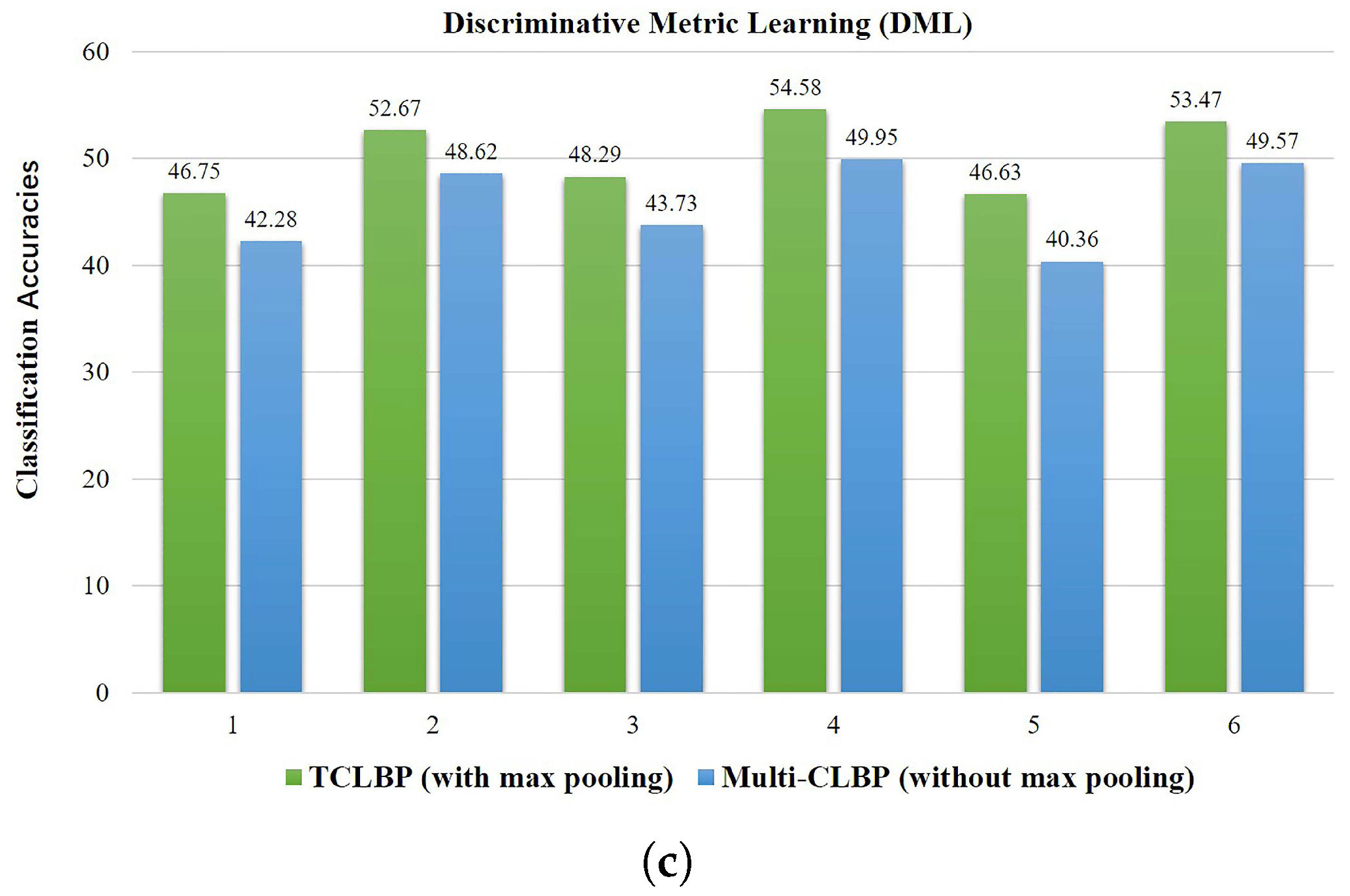
Figure 11.
Performance of the proposed methods under different m.
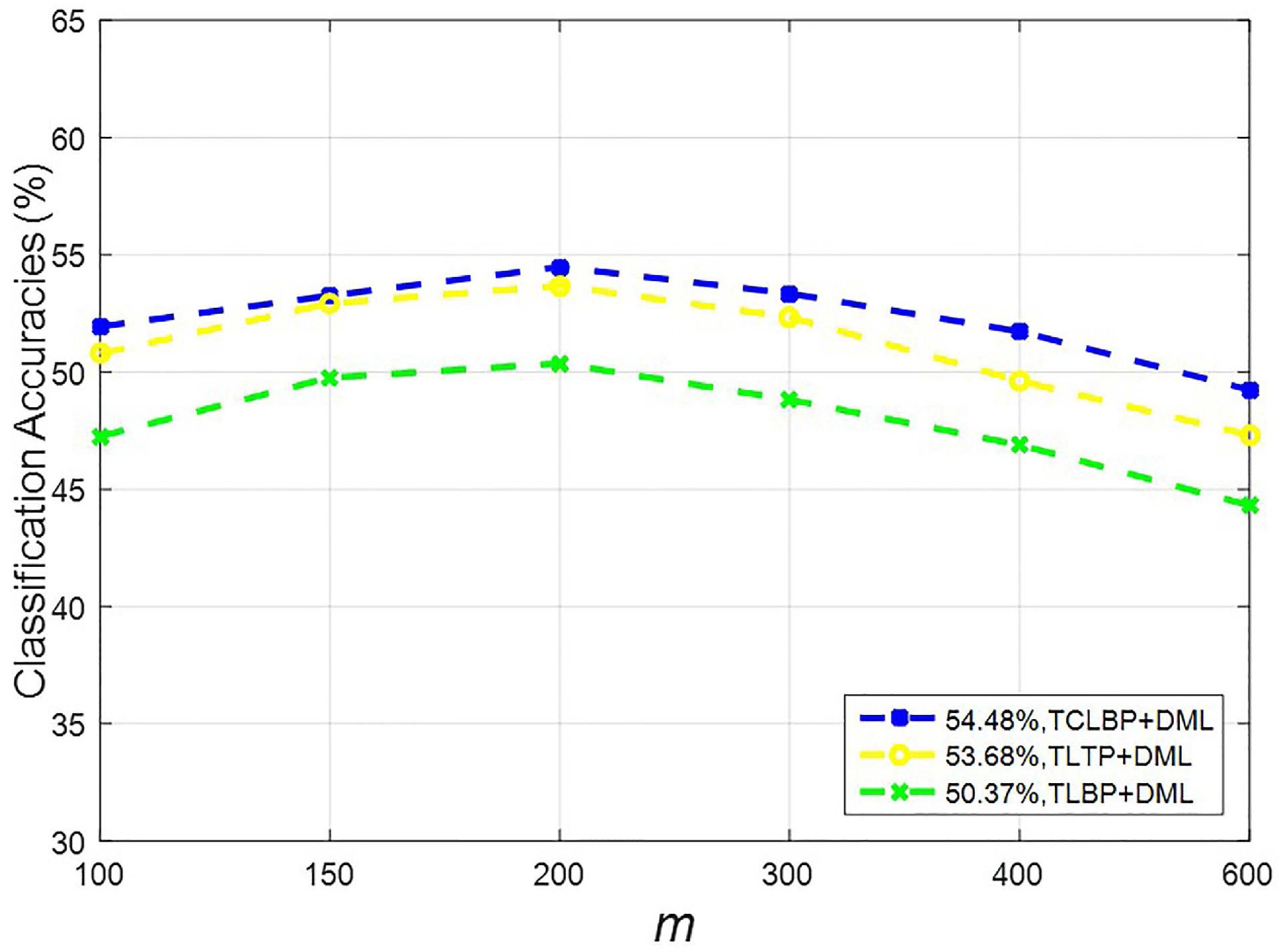
Figure 12.
Cross-domain recognition accuracy in the case of MOC to CAMS domain shift when a varying fraction of cloud images are from the target domain.
Figure 12.
Cross-domain recognition accuracy in the case of MOC to CAMS domain shift when a varying fraction of cloud images are from the target domain.

Table 1.
The genera types and descriptions according to WMO and the sample number in each class of three databases. The Arabic numbers are used to denote the cloud class label.
Table 1.
The genera types and descriptions according to WMO and the sample number in each class of three databases. The Arabic numbers are used to denote the cloud class label.
| Label | Cloud Genera | Number of Samples | Descriptions | ||
|---|---|---|---|---|---|
| CAMS | IAP | MOC | |||
| 1 | Cumulus | 378 | 316 | 187 | Low, puffy clouds with clearly defined edges, white or light-grey |
| 2 | Cirrus and cirrostratus | 261 | 353 | 191 | High, thin clouds, wisplike or sky covering, whitish |
| 3 | Cirrocumulus and altocumulus | 113 | 85 | 109 | High patched clouds of small cloudlets, mosaic-like, white |
| 4 | Clear sky | 171 | 102 | 224 | No clouds and cloudiness below 10% |
| 5 | Stratocumulus | 188 | 87 | 73 | Low or mid-level, lumpy layer of clouds, broken to almost overcast, white or grey |
| 6 | Stratus and altostratus | 190 | 200 | 390 | Low or mid-level layer of clouds, uniform, usually overcast, grey |
| 7 | Cumulonimbus and nimbostratus | 299 | 375 | 223 | Dark, thick clouds, mostly overcast, grey |
| Total number | 1600 | 1518 | 1397 | ||
Table 2.
The differences of three cloud databases.
| Location | Occlusion | Size [Pixels] | |
|---|---|---|---|
| CAMS | Yangjiang, Guangdong Province, China | No | |
| IAP | Yangjiang, Guangdong Province, China | Yes | |
| MOC | Wuxi, Jiangsu Province, China | Yes |
Table 3.
Cross-domain classification accuracies (%) with different local features. The three accuracy numbers in a triple are the basic classification accuracy, the recognition accuracy after IGC, and after FN, respectively.
Table 3.
Cross-domain classification accuracies (%) with different local features. The three accuracy numbers in a triple are the basic classification accuracy, the recognition accuracy after IGC, and after FN, respectively.
| Source | Target | LBP | TLBP | LTP | TLTP | CLBP | TCLBP |
|---|---|---|---|---|---|---|---|
| CAMS | IAP | (31.97, 35.51, | (34.53, 38.78, | (33.15, 37.41, | (37.42, 41.55, | (33.58, 37.94, | (39.76, 43.89, |
| 38.65) | 42.38) | 40.21) | 44.30) | 41.45) | 46.71) | ||
| CAMS | MOC | (37.43, 41.95, | (39.37, 44.19, | (41.52, 45.20, | (45.36, 49.87, | (41.85, 46.83, | (47.60, 52.18, |
| 44.80) | 47.73) | 48.26) | 53.45) | 49.81) | 55.69) | ||
| IAP | CAMS | (32.18, 36.47, | (35.31, 40.13, | (34.33, 38.26, | (39.60, 43.45, | (35.27, 39.79, | (41.58, 45.65, |
| 39.54) | 43.09) | 41.20) | 46.32) | 43.15) | 48.37) | ||
| IAP | MOC | (40.25, 45.61, | (43.82, 49.52, | (41.61, 46.37, | (47.23, 52.89, | (42.64, 47.56, | (47.92, 53.43, |
| 50.26) | 53.75) | 50.18) | 56.37) | 51.42) | 57.68) | ||
| MOC | CAMS | (30.14, 34.26, | (34.19, 38.34, | (32.68, 37.29, | (36.91, 40.78, | (33.06, 36.90, | (39.43, 43.75, |
| 36.71) | 41.12) | 39.82) | 43.92) | 39.43) | 45.84) | ||
| MOC | IAP | (39.76, 44.52, | (43.40, 48.63, | (41.64, 46.15, | (46.87, 51.64, | (42.12, 46.75, | (47.65, 52.40, |
| 48.37) | 52.38) | 49.73) | 55.26) | 50.84) | 56.15) |
Table 4.
Cross-domain classification accuracies (%) of local features with different metrics. The three accuracy numbers in a triple are the basic classification accuracy, the recognition accuracy after IGC, and after FN, respectively.
Table 4.
Cross-domain classification accuracies (%) of local features with different metrics. The three accuracy numbers in a triple are the basic classification accuracy, the recognition accuracy after IGC, and after FN, respectively.
| Source | Target | LBP | LTP | CLBP | ||||||
|---|---|---|---|---|---|---|---|---|---|---|
| Euclid | ML | DML | Euclid | ML | DML | Euclid | ML | DML | ||
| CAMS | IAP | (31.97, | (34.32, | (37.94, | (33.15, | (36.28, | (39.76, | (33.58, | (36.52, | (40.79, |
| 35.51, | 38.19, | 42.23, | 37.41, | 40.56, | 44.64, | 37.94, | 40.78, | 44.59, | ||
| 38.65) | 42.13) | 45.64) | 40.21) | 44.02) | 47.39) | 41.45) | 44.68) | 47.83) | ||
| CAMS | MOC | (37.43, | (39.29, | (42.23, | (41.52, | (42.03, | (47.16, | (41.85, | (44.15, | (48.20, |
| 41.95, | 44.15, | 46.90, | 45.20, | 46.82, | 51.75, | 46.83, | 48.96, | 52.87, | ||
| 44.08) | 48.01) | 51.23) | 48.26) | 50.46) | 55.37) | 49.81) | 52.53) | 55.42) | ||
| IAP | CAMS | (32.18, | (35.24, | (38.62, | (34.33, | (36.51, | (39.83, | (35.27, | (37.43, | (42.06, |
| 36.47, | 39.86, | 43.14, | 38.26, | 41.13, | 44.92, | 39.79, | 42.08, | 46.73, | ||
| 39.54) | 43.59) | 47.06) | 41.20) | 44.89) | 48.63) | 43.15) | 45.79) | 49.85) | ||
| IAP | MOC | (40.25, | (42.93, | (46.50, | (41.61, | (43.92, | (47.59, | (42.64, | (45.27, | (49.15, |
| 45.61, | 48.39, | 51.84, | 46.37, | 48.86, | 53.27, | 47.56, | 50.74, | 54.02, | ||
| 50.26) | 52.97) | 56.45) | 50.18) | 53.31) | 57.21) | 51.42) | 54.36) | 56.89) | ||
| MOC | CAMS | (30.14, | (33.64, | (37.81, | (32.68, | (36.24, | (38.45, | (33.06, | (36.38, | (40.62, |
| 34.26, | 37.87, | 41.65, | 37.29, | 40.15, | 42.21, | 36.90, | 40.10, | 44.25, | ||
| 36.71) | 40.83) | 44.69) | 39.82) | 43.60) | 45.38) | 39.43) | 44.25) | 47.46) | ||
| MOC | IAP | (39.76, | (42.25, | (45.09, | (41.64, | (43.59, | (47.24, | (42.12, | (44.70, | (48.23, |
| 44.52, | 47.56, | 50.07, | 46.15, | 48.71, | 52.29, | 46.75, | 49.82, | 53.12, | ||
| 48.37) | 51.92) | 54.43) | 49.73) | 52.56) | 56.42) | 50.84) | 52.67) | 56.75) | ||
Table 5.
Cross-domain classification accuracies (%) of transferred local features with different metrics. The three accuracy numbers in a triple are the basic classification accuracy, the recognition accuracy after IGC, and after FN, respectively.
Table 5.
Cross-domain classification accuracies (%) of transferred local features with different metrics. The three accuracy numbers in a triple are the basic classification accuracy, the recognition accuracy after IGC, and after FN, respectively.
| Source | Target | TLBP | TLTP | TCLBP | ||||||
|---|---|---|---|---|---|---|---|---|---|---|
| Euclid | ML | DML | Euclid | ML | DML | Euclid | ML | DML | ||
| CAMS | IAP | (34.53, | (38.34, | (42.10, | (37.42, | (39.95, | (44.12, | (39.76, | (39.76, | (46.75, |
| 38.78, | 42.59, | 45.96, | 41.55, | 44.29, | 48.37, | 43.89, | 47.72, | 51.14, | ||
| 42.38) | 46.10) | 49.25) | 44.30) | 46.74) | 51.82) | 46.71) | 50.41) | 53.85) | ||
| CAMS | MOC | (39.37, | (43.13, | (47.89, | (45.36, | (47.32, | (51.24, | (47.60, | (48.85, | (52.67, |
| 44.19, | 45.98, | 53.02, | 49.87, | 50.83, | 55.94, | 52.18, | 53.76, | 57.29, | ||
| 47.73) | 49.38) | 55.46) | 53.45) | 54.57) | 59.35) | 55.69) | 56.37) | 60.51) | ||
| IAP | CAMS | (35.31, | (38.96, | (43.24, | (39.60, | (42.34, | (45.91, | (41.58, | (43.56, | (48.29, |
| 40.13, | 43.67, | 47.51, | 43.45, | 47.62, | 49.71, | 45.65, | 48.19, | 51.90, | ||
| 43.09) | 47.92) | 51.17) | 46.32) | 50.81) | 52.58) | 48.37) | 51.64) | 54.59) | ||
| IAP | MOC | (43.82, | (47.65, | (50.37, | (47.23, | (49.70, | (53.68, | (47.92, | (50.74, | (54.58, |
| 49.52, | 52.46, | 55.23, | 52.89, | 54.37, | 59.50, | 53.43, | 55.94, | 59.71, | ||
| 53.75) | 55.31) | 59.48) | 56.37) | 57.12) | 63.24) | 57.68) | 59.40) | 64.28) | ||
| MOC | CAMS | (34.19, | (38.21, | (42.03, | (36.91, | (39.76, | (43.97, | (39.43, | (42.28, | (46.63, |
| 38.34, | 42.13, | 45.58, | 40.78, | 44.02, | 47.86, | 43.75, | 46.63, | 50.94, | ||
| 41.12) | 45.76) | 48.59) | 43.92) | 46.48) | 50.69) | 45.84) | 49.21) | 52.63) | ||
| MOC | IAP | (43.40, | (45.97, | (49.58, | (46.87, | (49.18, | (52.93, | (47.65, | (50.13, | (53.47, |
| 48.63, | 51.09, | 53.42, | 51.64, | 53.71, | 57.68, | 52.40, | 54.82, | 57.42, | ||
| 52.38) | 54.60) | 57.13) | 55.26) | 56.85) | 62.43) | 56.15) | 57.64) | 61.57) | ||
Table 6.
After IGC and FN, cross-domain classification accuracies (%) of concatenating the TLBP, TLTP and TCLBP to form a feature vector for representing the cloud image with different metrics.
Table 6.
After IGC and FN, cross-domain classification accuracies (%) of concatenating the TLBP, TLTP and TCLBP to form a feature vector for representing the cloud image with different metrics.
| Source | Target | TLBP + TLTP + TCLBP | ||
|---|---|---|---|---|
| Euclid | ML | DML | ||
| CAMS | IAP | 54.83 | 57.64 | 62.12 |
| CAMS | MOC | 62.90 | 64.25 | 68.37 |
| IAP | CAMS | 55.21 | 58.92 | 62.45 |
| IAP | MOC | 65.32 | 67.83 | 72.91 |
| MOC | CAMS | 53.70 | 57.10 | 60.28 |
| MOC | IAP | 63.69 | 65.83 | 70.56 |
Table 7.
After IGC, FN, and the concatenation of the TLBP, TLTP and TCLBP, cross-domain classification accuracies (%) of CSM with different metrics.
Table 7.
After IGC, FN, and the concatenation of the TLBP, TLTP and TCLBP, cross-domain classification accuracies (%) of CSM with different metrics.
| Source | Target | CSM + TLBP + TLTP + TCLBP | ||
|---|---|---|---|---|
| Euclid | ML | DML | ||
| CAMS | IAP | 74.63 | 75.96 | 80.45 |
| CAMS | MOC | 78.57 | 80.90 | 82.13 |
| IAP | CAMS | 73.25 | 76.61 | 80.38 |
| IAP | MOC | 80.71 | 82.47 | 85.62 |
| MOC | CAMS | 72.74 | 74.52 | 78.81 |
| MOC | IAP | 79.82 | 81.76 | 84.29 |
Table 8.
Cross-domain classification accuracies (%) comparing our method with state-of-the-art methods.
Table 8.
Cross-domain classification accuracies (%) comparing our method with state-of-the-art methods.
| Source | Target | BoW | MRP | TCLBP + DML | CSM + (TLBP + TLTP + TCLBP) + DML | ||
|---|---|---|---|---|---|---|---|
| The Basic | With IGC | With IGC and FN | |||||
| CAMS | IAP | 33.26 | 34.13 | 46.75 | 51.14 | 53.85 | 80.45 |
| CAMS | MOC | 38.27 | 40.06 | 52.67 | 57.29 | 60.51 | 82.13 |
| IAP | CAMS | 33.75 | 34.21 | 48.29 | 51.90 | 54.59 | 80.38 |
| IAP | MOC | 40.86 | 43.13 | 54.58 | 59.71 | 64.28 | 85.62 |
| MOC | CAMS | 30.98 | 32.75 | 46.63 | 50.94 | 52.63 | 78.81 |
| MOC | IAP | 40.35 | 42.94 | 53.47 | 57.42 | 61.57 | 84.29 |
© 2017 by the authors. Licensee MDPI, Basel, Switzerland. This article is an open access article distributed under the terms and conditions of the Creative Commons Attribution (CC BY) license (http://creativecommons.org/licenses/by/4.0/).
Share and Cite
MDPI and ACS Style
Zhang, Z.; Li, D.; Liu, S.; Xiao, B.; Cao, X. Cross-Domain Ground-Based Cloud Classification Based on Transfer of Local Features and Discriminative Metric Learning. Remote Sens. 2018, 10, 8. https://doi.org/10.3390/rs10010008
AMA Style
Zhang Z, Li D, Liu S, Xiao B, Cao X. Cross-Domain Ground-Based Cloud Classification Based on Transfer of Local Features and Discriminative Metric Learning. Remote Sensing. 2018; 10(1):8. https://doi.org/10.3390/rs10010008
Chicago/Turabian StyleZhang, Zhong, Donghong Li, Shuang Liu, Baihua Xiao, and Xiaozhong Cao. 2018. "Cross-Domain Ground-Based Cloud Classification Based on Transfer of Local Features and Discriminative Metric Learning" Remote Sensing 10, no. 1: 8. https://doi.org/10.3390/rs10010008
Note that from the first issue of 2016, this journal uses article numbers instead of page numbers. See further details here.