Object-Based Mangrove Species Classification Using Unmanned Aerial Vehicle Hyperspectral Images and Digital Surface Models

Abstract

Mangroves are one of the most important coastal wetland ecosystems, and the compositions and distributions of mangrove species are essential for conservation and restoration efforts. Many studies have explored this topic using remote sensing images that were obtained by satellite-borne and airborne sensors, which are known to be efficient for monitoring the mangrove ecosystem. With improvements in carrier platforms and sensor technology, unmanned aerial vehicles (UAVs) with high-resolution hyperspectral images in both spectral and spatial domains have been used to monitor crops, forests, and other landscapes of interest. This study aims to classify mangrove species on Qi’ao Island using object-based image analysis techniques based on UAV hyperspectral images obtained from a commercial hyperspectral imaging sensor (UHD 185) onboard a UAV platform. First, the image objects were obtained by segmenting the UAV hyperspectral image and the UAV-derived digital surface model (DSM) data. Second, spectral features, textural features, and vegetation indices (VIs) were extracted from the UAV hyperspectral image, and the UAV-derived DSM data were used to extract height information. Third, the classification and regression tree (CART) method was used to selection bands, and the correlation-based feature selection (CFS) algorithm was employed for feature reduction. Finally, the objects were classified into different mangrove species and other land covers based on their spectral and spatial characteristic differences. The classification results showed that when considering the three features (spectral features, textural features, and hyperspectral VIs), the overall classification accuracies of the two classifiers used in this paper, i.e., k-nearest neighbor (KNN) and support vector machine (SVM), were 76.12% (Kappa = 0.73) and 82.39% (Kappa = 0.801), respectively. After incorporating tree height into the classification features, the accuracy of species classification increased, and the overall classification accuracies of KNN and SVM reached 82.09% (Kappa = 0.797) and 88.66% (Kappa = 0.871), respectively. It is clear that SVM outperformed KNN for mangrove species classification. These results also suggest that height information is effective for discriminating mangrove species with similar spectral signatures, but different heights. In addition, the classification accuracy and performance of SVM can be further improved by feature reduction. The overall results provided evidence for the effectiveness and potential of UAV hyperspectral data for mangrove species identification.

1. Introduction

Mangroves are one of the most important objects in wetland ecosystems. They usually thrive in the mud flats of estuarine regions along tropical and subtropical coastlines [1]. They are ecologically and socioeconomically significant because of their important ecological roles in reducing coastal erosion, storm protection, flood and flow control, and water quality control, etc. [2]. However, during the past century, mangrove forests have been in serious decline [3,4]. Accurate mangrove species classification is an essential component of mangrove forest inventories and wetland ecology management, etc. Therefore, there is an emerging demand for conservation and restoration initiatives that contribute to mangrove monitoring.

Remote sensing techniques are known to be fast and efficient for monitoring the mangrove ecosystem when compared with conventional field work, which is costly, time-consuming, and sometimes impossible due to the poor accessibility of mangrove areas. In previous studies, multi-spectral sensors on satellite platforms such as Landsat TM [5] and SPOT XS [6], have been mostly used for mangrove mapping at global or regional scales [7,8]. Due to poor spatial or spectral resolution of these traditional multi-spectral images, they have been rarely used for mangrove species classification. With the development of high-spatial resolution satellite sensors, such as IKONOS [9,10], Quickbird [11,12], and WorldView-2 [13,14], their high-spatial resolution images are gradually used to identify mangrove species because of their detailed spatial characteristics, such as textural structure.

Hyperspectral imaging technology plays an important role in improving the ability to differentiate tree species composition [15]. With imaging spectrometers, hyperspectral images can provide abundant spectral information with hundreds of narrow bands and a continuous spectral profile for each pixel, which can greatly increase the amount of detailed information available on land covers [16,17]. Many papers have been published on the use of hyperspectral data acquired by various satellite-borne or airborne sensors in mangrove mapping. Hirano et al. used AVIRIS hyperspectral image data to produce a wetland vegetation map, but the overall map accuracy was only 66% due to inadequate spatial resolution and a lack of stereo viewing [18]. Koedsin and Vaiphasa discriminated five mangrove species using EO-1 Hyperion hyperspectral images and refined the classification outcome using differences in leaf textures [19]. Jia et al. combined EO-1 Hyperion hyperspectral images and high-spatial-resolution SPOT-5 data to map mangrove species using an object-based method. The classification results indicated the great potential of using high-resolution hyperspectral data for distinguishing and mapping mangrove species [20]. Kamal and Phinn verified the effectiveness of high-spatial-resolution CASI-2 hyperspectral images for mapping mangrove species [21]. According to these previous studies, hyperspectral images can provide rich spectral information, but for fine classification of tree species, which relies only on spectral characteristics, classification effectiveness is still limited. As an important complementary feature, incorporation of spatial structure information makes it possible to classify tree species on a finer scale [22,23].

Based on the development of sensor technology and remote sensing platforms, more accurate and timely satellite images with high spectral and spatial resolutions, which have a positive impact on identification accuracy [24], can be easily acquired. Unmanned aerial vehicles (UAVs), as emerging unmanned aircraft systems, are increasingly being used as remote sensing platforms [25]. Furthermore, hyperspectral sensors have been shrinking in size and weight, and their use onboard of UAVs has become feasible [26,27,28]. Recently, several studies have addressed the use of UAV hyperspectral sensors in vegetation [29,30], crop [31,32,33,34,35,36,37,38,39,40,41,42], forest monitoring [43], and wetland species mapping [44], etc. However, few specific results have been published on mapping mangrove species using UAV hyperspectral images.

Most studies on mangrove species classification were conducted using pixel-based methods such as spectral angle mapper (SAM) [45,46], maximum likelihood classification (MLC) [7,8,46], and spectral unmixing [47,48,49], or object-based methods, such as nearest neighbor (NN) [20,21], random forest (RF) [50], and support vector machine (SVM) [14,51,52]. Previous studies have shown that the object-based methods generally outperformed the pixel-based methods for mangrove species classification, particularly with high-resolution hyperspectral images [21,53,54,55]. For most object-based classifications, the spectral features were widely used [56], but spatial or structural information like textures and morphological characteristics was also considered. Canopy height is also considered as an important variable in tree species mapping and has been generated using LiDAR, SAR, and UAV data, etc. From previous studies, incorporation of canopy height into a tree species or crop species classification can improve classification accuracy [50,57]. Nevertheless, only a few studies have taken canopy height into account for mangrove classification by integrating LiDAR and multispectral images [58,59]. Canopy height is rarely used in mangrove species classification based on hyperspectral images. In addition, a low-cost camera onboard a UAV platform can be used to obtain tree height [4,60]. When compared to LiDAR, the acquisition of UAV images is simpler, faster, and less expensive.

The main objectives of this study are: (1) to investigate the capability of UAV hyperspectral images for distinguishing and mapping mangrove species using object-based approaches on Qi’ao Island; and, (2) to determine the importance of height information in mangrove species classification. This study also analyzes the differences in accuracy of mangrove species mapping with different features and methods.

The rest of this paper is organized as follows. Section 2 describes the study area and the dataset used in the experiments. Section 3 presents the methods for image segmentation, feature extraction and selection, and object-based classification. Section 4 analyzes and discusses the experimental results. Finally, Section 5 presents a summary of the entire study and the conclusions.

2. Study Area and Data

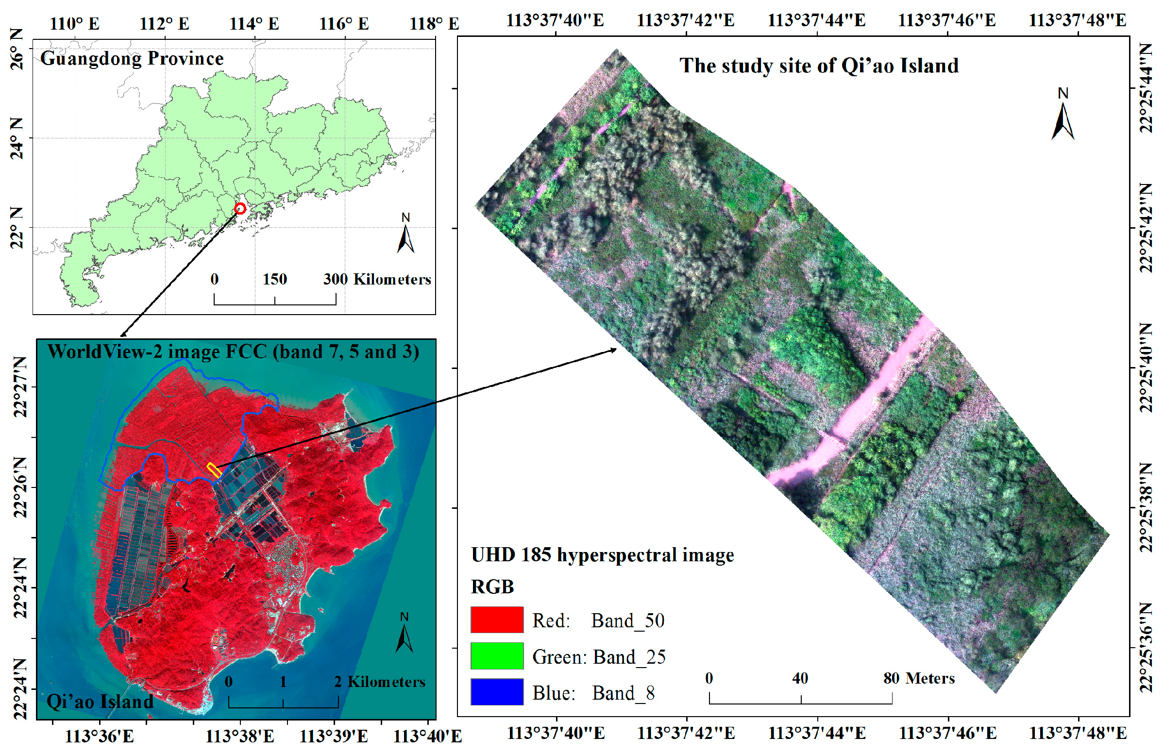
2.1. Study Area

The Qi’ao Island mangrove nature reserve is situated in northwestern Dawei Bay on Qi’ao Island (22°23′40″–22°27′38″N, 113°36′40″–113°39′15″E), Zhuhai City, Guangdong Province, China (see blue boundary at lower left of Figure 1). Qi’ao Island is the most complete preservation area and the most concentrated forest stand in Zhuhai City. As a mangrove plant gene pool and the main breeding ground of migratory birds in the Pearl River Delta, it is also an important typical-subtropical mangrove wetland ecological ecosystem in the coastal area of southeastern China [14]. Qi’ao Island has the largest artificially restored mangrove area in China, covering an area of approximately 700 ha [13]. In this study, due to the acquisition range of the UAV hyperspectral data, a subset of the study area is chosen as the study site, as shown in the right portion of Figure 1.

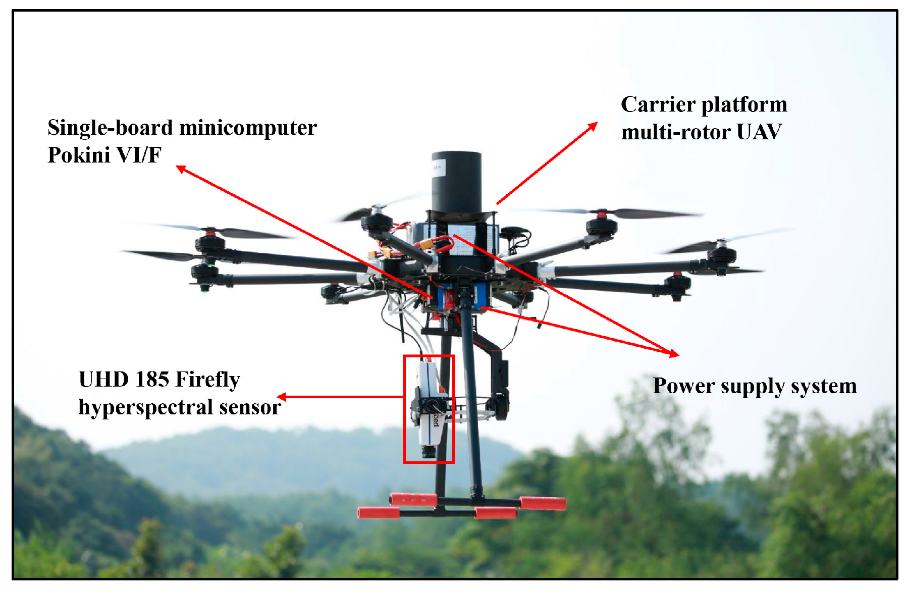
2.2. UAV Hyperspectral Data Acquisition

A high-spatial-resolution hyperspectral image, collected from a commercial UHD 185 hyperspectral sensor onboard of a multi-rotor UAV platform, was used in this study. The high spatial and spectral resolution of the UAV hyperspectral image makes it possible to distinguish different mangrove species. The hyperspectral imaging system (Figure 2) consisted of a Cubert UHD 185 hyperspectral sensor (http://cubert-gmbh.de/) and a Pokini VI/F single-board minicomputer (http://www.pokini.de/). The UHD 185 hyperspectral sensor can capture 138 spectral bands with a spectral interval of 4 nm, covering the 450–998 nm spectral region. Following the approach that was used in previous researches [26,36], 125 bands between 454 and 950 nm were used in this paper. For each band, a 50 × 50 image cube with 12-bit radiometric resolution was created. The image capture task was conducted at an altitude of 80 m on 15 October 2016, under cloudless conditions at noontime. The hyperspectral data were acquired with approximately 0.02 m spatial resolution. In Figure 1, the yellow border represents the extent of the data acquisition area, approximately 3 ha. This subset of the UAV hyperspectral image covering the study site was used in this research.

2.3. Image Preprocessing

More than 1000 UHD 185 hyperspectral cubes were acquired by the hyperspectral imaging system. After removing the cubes corresponding to the takeoff and landing of the UAV, 625 of the original hyperspectral cubes were used for image fusion, based on the references by [38,39,61]. Each hyperspectral cube and its corresponding panchromatic image were fused using a Cubert-Pilot software (Cubert GmbH, Ulm, Baden-Württemberg, Germany). The entire UAV hyperspectral image of the study site was stitched together by fusing hyperspectral images based on the point clouds of the panchromatic image with automatic image mosaic software, known as Agisoft PhotoScan (Agisoft, St. Petersburg, Russia).

The UAV hyperspectral image was radiometrically corrected with reference measurements on a white board and dark measurements by covering the black plastic lens cap. To obtain the reflectance values, the dark measurements were subtracted from the reference measurements and the actual measured values [28]. After radiometric calibration, the UAV hyperspectral image was geometrically corrected with reference to another UAV image that was acquired on 11 September 2015, based on the image-to-image method. The UAV hyperspectral image with 0.02 m spatial resolution was resampled into 0.15 m spatial resolution using a nearest-neighbor resampling method. Because of the flat terrain of the study site, digital surface model (DSM) features obtained from the UAV image using ENVI LiDAR 5.3 were expected to provide relative height differentiation between different mangrove species for this study. According to previous studies [60], DSM data obtained from high-resolution images acquired with UAV can be used in the context of tree height quantification.

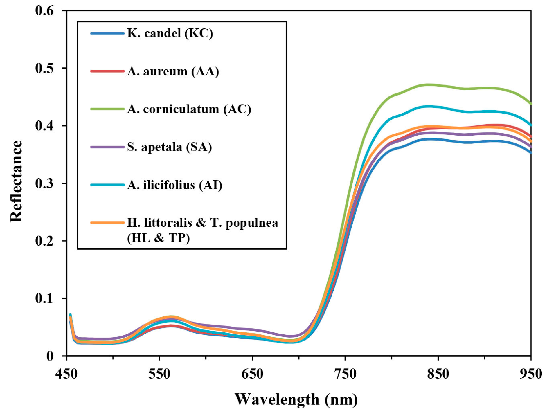
2.4. Field Surveys and Sample Collection

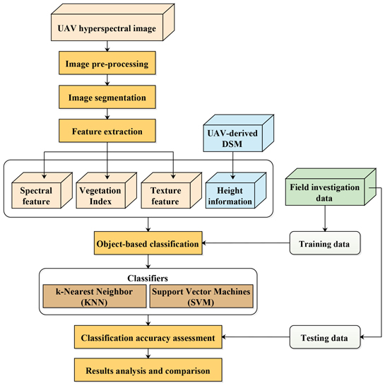
To survey the characteristics and spatial distribution of mangrove species in the study site, three field investigations were carried out on 1–3 July 2016, 1 January 2017, and 6–8 June 2017, on Qi’ao Island. A handheld GPS device (Garmin 629sc) was used to record the precise locations of mangrove samples, and then these locations were verified with a UAV image and a WorldView-2 image, acquired on 11 September 2015, and 18 October 2015, respectively. According to these field investigations, in the study site, the primary mangrove species included K. candel (KC), A. aureum (AA), A. corniculatum (AC), S. apetala (SA), A. ilicifolius (AI), H. littoralis (HL), and T. populnea (TP). KC and SA were the dominant mangrove species, and other mangrove species were fairly scattered over the study site. SA stands have taller tree height; in contrast, AA and AI stands are shorter and are generally classed as undergrowth. KC in the study site includes prevalent mature stands and some stands that were artificially restored in recent years. AC tends to occur with AI. HL and TP are slightly shorter than SA and are generally mixed. The other three land covers include herbaceous vegetation, such as P. australis (PA), water area (river), and boardwalks. Due to changes in solar elevation angle, there are some shadows on the UAV hyperspectral images. In this study, they were considered as a single class in the object-based classification.

Reference data were collected from the UAV image, the WorldView-2 image, and field observations that are verified by local experts. As a result, 828 ground truth samples were randomly selected (

Table 1. Number of ground investigation points.

Land-Cover Types	Ground Truth Samples		Total
	Training Samples	Testing Samples
K. candel (KC)	68	58	126
A. aureum (AA)	46	31	77
A. corniculatum (AC)	37	45	82
S. apetala (SA)	71	41	112
A. ilicifolius (AI)	28	22	50
H. littoralis & T. populnea (HL & TP)	60	41	101
water area (river)	93	40	133
P. australis (PA)	22	18	40
boardwalk	14	10	24
shadow	54	29	83
total	493	335	828

). These samples were then randomly divided into two groups for object-based classification (493 training samples) and validation (335 testing samples).

The mean reflectance spectra of six mangrove species were obtained from the ground truth samples based on the UAV hyperspectral image. The general shapes of these mangrove species’ curves are very similar, with considerable overlap (Figure 3). Bands within the 550-nm spectral region, and from 750 to 950 nm are different from each other, which is mainly due to differences in pigment content, such as chlorophyll content, and in internal leaf structure.

In addition, the mean heights for six mangrove species were calculated from the UAV-derived DSM, as shown in Figure 4a,b. It is clear that the SA stands are generally the highest in the study site, whereas the AA, the AC, and the AI stands have similar mean heights and the KC, HL, and TP stands are also similar. These results are consistent with the field investigations and previous studies [62,63].

3. Methods

In this study, a UAV hyperspectral image was used for object-based mangrove species classification. The classification procedure consisted of four steps: (1) selection of the optimal segmentation parameters and image segmentation; (2) object feature extraction from the UAV hyperspectral image and the UAV-derived DSM data, band selection using CART, feature selection using CFS with the best first search algorithm; (3) object-based classification using KNN and SVM; and, (4) classification accuracy assessment with overall accuracy (OA), kappa coefficient (Kappa), and confusion matrices. Figure 5 shows the flowchart of object-based mangrove species classification based on the UAV hyperspectral image.

3.1. Image Segmentation

Image segmentation is the first step of object-based image analysis and is used to generate image objects that are more homogeneous among themselves than with nearby regions [64]. The accuracy of image segmentation significantly influences object-based classification accuracy [65]. The most widely used multi-resolution segmentation, a bottom up region-merging technique [66], was used to generate image objects. This method requires three primary segmentation parameters: scale, shape, and compactness. In this study, a series of interactive “trial and error” tests were applied to determine the proper segmentation parameters [67]. All of the image processing procedures for object-based classification were carried out using eCognition Developer 9.0 software (Trimble Germany GmbH, Munich, Germany).

3.2. Feature Extraction and Selection

Object-based classification was developed as a means of incorporating hierarchical spectral and spatial features into an image mapping procedure. Features associated with the image objects can be derived from the image segmentation. The ideal features should present the highest separability of the targeted objects, which means that they have the highest within-class similarity and the lowest inter-class overlap. Due to similar spectral responses between different mangrove species, it is necessary to integrate spectral and spatial information to achieve accurate mapping.

In this study, four sets of features were evaluated, as listed in

Table 2. Object features used for classification.

Object Features	Description
spectral bands	Mean values of 125 spectral bands for each image object, brightness, and max.diff.
hyperspectral vegetation indices (vis)	Eight VIs, including BGI2, NDVI, RDVI, TCARI, OSAVI, TCARI/OSAVI, MCARI2, and PRI.
textural features	24 textural features, including ASM, CON, COR, ENT, HOM, MEAN, DIS, StdDev calculated using GLCM with three bands (that is band 8, band 25, and band 50).
height information	UAV-derived DSM (Digital Surface Model).

. (1) Spectral bands, including 125 hyperspectral bands (mean values), brightness, and max.diff (maximum intensity difference), were considered. (2) Hyperspectral vegetation indices (VIs), or narrow-band VIs, which can generally be considered as an extension of spectral features, were also included. Eight VIs (

Table 3. Vegetation Indices (VIs) derived from hyperspectral bands.

Hyperspectral Vegetation Indices (VIs)	Formulation
Blue Green Pigment Index 2 (BGI 2)	$\mathrm{BGI}2={\mathsf{\rho }}_1/{\mathsf{\rho }}_{25}$
Normalized Difference Vegetation Index (NDVI)	$\mathrm{NDVI}=\left({\mathsf{\rho }}_{87} - {\mathsf{\rho }}_{55}\right)/\left({\mathsf{\rho }}_{87}{+\mathsf{\rho }}_{55}\right)$
Reformed Difference Vegetation Index (RDVI)	$\mathrm{RDVI}=\left({\mathsf{\rho }}_{87} - {\mathsf{\rho }}_{55}\right)/\left(\sqrt{{\mathsf{\rho }}_{87}{+\mathsf{\rho }}_{55}}\right)$
Transformed Chlorophyll Absorption in Reflectance Index (TCARI)	$\mathrm{TCARI}=3\left[\left({\mathsf{\rho }}_{63} - {\mathsf{\rho }}_{55}\right)-0.2\left({\mathsf{\rho }}_{63} - {\mathsf{\rho }}_{25}\right)\text{×}\left({\mathsf{\rho }}_{63}/{\mathsf{\rho }}_{55}\right)\right]$
Optimized Soil-Adjusted Vegetation Index (OSAVI)	$\mathrm{OSAVI}=\left(1+0.16\right)\text{×}\left({\mathsf{\rho }}_{87} - {\mathsf{\rho }}_{55}\right)/\left({\mathsf{\rho }}_{87}{+\mathsf{\rho }}_{55}+0.16\right)$
TCARI/OSAVI	$\mathrm{TCARI}/\mathrm{OSAVI}$
Modified Chlorophyll Absorption Ratio Index 2 (MCARI 2)	$\mathrm{MCARI}2=\frac{1.5\left[2.5\left({\mathsf{\rho }}_{87} - {\mathsf{\rho }}_{55}\right) - 1.3\left({\mathsf{\rho }}_{87}-{\mathsf{\rho }}_{25}\right)\right]}{\sqrt{{\left({2\mathsf{\rho }}_{87}+1\right)}^2 - \left({6\mathsf{\rho }}_{87} - 5\sqrt{{\mathsf{\rho }}_{55}}\right) - 0.5}}$
Photo-chemical Reflectance Index (PRI)	$\mathrm{PRI}=\left({\mathsf{\rho }}_{16} - {\mathsf{\rho }}_{20}\right)/\left({\mathsf{\rho }}_{16}{+\mathsf{\rho }}_{20}\right)$

Note: these parameters, from ρ1 to ρ125, correspond respectively to the 125 bands between 454 nm and 950 nm of the UHD 185 hyperspectral image.

) that were frequently used in previous studies [26] were chosen, including transformed chlorophyll absorption in reflectance index (TCARI) [68], optimized soil-adjusted vegetation index (OSAVI) [69], TCARI/OSAVI [68], blue green pigment index 2 (BGI2) [70], photochemical reflectance index (PRI) [71], normalized difference vegetation index (NDVI) [72], reformed difference vegetation index (RDVI) [73], and modified chlorophyll absorption ratio index (MCARI 2) [74]. (3) Textural feature is an important factor in object-based classification. It generally reflects local spatial information that is related to tonal variations in the image. Various statistical methods have been employed to derive textural features, the grey level co-occurrence matrix (GLCM) being the most popular [75,76].

Table 4. Grey level co-occurrence matrix (GLCM)-derived second-order textural measures and their corresponding equations.

Textural Variables	Formulation
ASM (Angular Second Moment)	$\mathrm{ASM}={\displaystyle \sum _i}{\displaystyle \sum _j}P{\left[i,j\right]}^2$
CON (Contrast)	$\mathrm{CON}={\displaystyle \sum _i}{\displaystyle \sum _j}P{\left(i-j\right)}^{2}P\left[i,j\right]$
COR (Correlation)	$\mathrm{COR}=\frac{{\sum }_i{\sum }_{j}ijP\left[i,j\right]-{\mu }_i{\mu }_j}{{\sigma }_i{\sigma }_j}$
ENT (Entropy)	$\mathrm{ENT}=-{\displaystyle \sum _i}{\displaystyle \sum _j}P\left[i,j\right]\mathrm{In}P\left[i,j\right]$
HOM (Homogeneity)	$\mathrm{HOM}={\displaystyle \sum _i}{\displaystyle \sum _j}\frac{P\left[i,j\right]}{1+{\left(i-j\right)}^2}$
Mean	${\mu }_i={\displaystyle \sum }ip[i,j]$
DIS (Dissimilarity)	$\mathrm{DIS}={\displaystyle \sum _i}{\displaystyle \sum _j}P\left|i,j\right|$
StdDev (Standard Deviation)	${\sigma }_i{}^2={\displaystyle \sum }{i}^{2}p[i,j]-{\mu }_i{}^2$

Note: $i$ is the row number of the image; $j$ is the column number of the image; $P[i,j]$ represents the relative frequency of two neighboring pixels.

lists eight second-order textural measures calculated using GLCM, including angular second moment (ASM), contrast (CON), correlation (COR), entropy (ENT), homogeneity (HOM), mean, dissimilarity (DIS), and StdDev (Standard Deviation), which are commonly used for object-based classification. According to two previous studies [26,77], three bands of the UAV hyperspectral image, i.e., B₄₈₂, G₅₅₀, and R₆₅₀, were selected to obtain the textural variables. A total of 24 object-based textural features were generated. (4) Due to the flat terrain of the study site, the DSM was extracted from the UAV image to determine relative height information for mangrove species with respect to the ground. These features were subsequently integrated by means of vector stacking and were considered as initial input variables to train and construct the classification models (the KNN and SVM classifiers) to classify the UAV hyperspectral image.

To reduce the redundant bands of hyperspectral datasets for this study, classification and regression tree (CART) was selected. CART is a non-parametric [78] and binary decision tree algorithm. CART can provide stable performance and reliable results in machine learning and data mining research [79]. It can be used to identify spectral bands with the highest discriminative capabilities between classes. Previous research has shown that CART can be used to identify those spectral bands which result in small misclassification rates [80]. Furthermore, the correlation-based feature selection (CFS) [81] with the best first search algorithm [82] was used to further select the most effective features for this study [83]. CFS has been reported to be an effective tool to select the optimal feature subset from complex remote sensing datasets [84]. As a classic filter feature selection mode, CFS calculates the feature-class and feature-feature correlation matrices based on the training set, and then search the feature subset using the best first search algorithm based on the redundancy between features. In this study, the full training set was used for feature selection. The procedures of CART and CFS were performed in Weka.

3.3. Object-Based Classification

The object-based classification method has been widely used and has proved to be more accurate and robust than the traditional pixel-based method, which relies solely on spectral information and tends to be affected by the salt-and-pepper effect [85]. In our experiments, the image objects acquired by image segmentation were used as the object-based classification unit, and the object features extracted from the UAV hyperspectral data and the UAV-derived DSM are considered as the classification criteria. Two classifiers, KNN and SVM, were chosen for object-based mangrove species classification.

3.3.1. KNN

KNN is an instance-based learning method [86,87], and is generally considered as one of the simplest machine learning classifiers. It has been widely used for high-resolution and hyperspectral image classification [21,88]. KNN is defined to classify objects based on the closest training samples in the feature space. The distance between each unknown object and its k nearest neighbors can be measured. If most of the k neighboring samples of the unknown object belongs to one class, this object can be placed in the same class. Therefore, the neighborhood value k is a key parameter of the KNN classifier, which significantly determines the classification result. Through multiple testing with the training samples of different feature subsets, the optimal neighborhood value k of each KNN object-based classification experiment was determined.

3.3.2. SVM

SVM is an advanced supervised non-parametric classifier that has been extensively used for hyperspectral image classification [76,89,90], including mangrove species classification [51,52]. Based on statistical learning theory, SVM is designed to look for an optimal decision hyperplane in high-dimensional space, which produces an optimal separation of classes. For ill-posed classification problems with high-dimensional features, SVM always gives good performance, even with a limited number of training samples. For the SVM classifier, the radial basis function (RBF) kernel was chosen because it has been proven to be superior to other kernels, especially for high-dimensional classification features. The SVM classifier has two important tuning parameters, cost of constraints (C) and sigma (σ), which have a great impact on classification accuracy. Before the SVM classifier was trained, the optimal input parameters were determined by a grid search strategy using the LIBSVM 3.22 library [91]. Finally, for the SVM object-based classification experiments, the optimal parameter values were derived from the training samples of different feature subsets.

3.4. Classification Accuracy Assessment

To assess the accuracy of the classification results from the KNN and SVM classifiers and to evaluate the effectiveness of the UAV hyperspectral data in mangrove species classification, confusion matrices were created using the 335 testing samples, which were considered as ground truth. For each of the classification results, the confusion matrix provides the OA, the Kappa, the user’s accuracy (UA), and the producer’s accuracy (PA) [92].

4. Results and Discussion

4.1. Analysis of Image Segmentation Results

The subsets of the UAV hyperspectral image used for this study were segmented with different scale factors, shape indices, and compactness parameters, as shown in Figure 6. (1) The segmentation scale is a critical image segmentation parameter because it determines the maximum allowed heterogeneity for the resulting image objects based on image features. With the default shape index (0.1) and compactness (0.5), the scale was set to 150, 100, 50, and 20 in separate tests (Figure 6a). When the segmentation scale was defined as 150, neighboring objects with similar features were generally mixed together, for example, AA and PA. When the scale was set to 50 or 20, the segmentation results were too fragile, which would influence the efficiency of image processing. Hence, a scale of 100 was used to create homogeneous segments. (2) According to the defined scale (100) and the default compactness (0.5), the shape index was set to 0.1, 0.3, 0.4, and 0.5 in separate tests (Figure 6b). When the shape index was defined as 0.1, 0.3, and 0.4, adjacent objects with a certain degree of shape similarity were combined into one class, such as the boardwalks and the water area (river). Through several interactive tests, the shape index was set to 0.5 to create meaningful objects. (3) With the defined scale (100) and shape index (0.5), the compactness was set to 0.3, 0.5, 0.7, and 0.9 in separate tests (Figure 6c). Based on visual inspection of the segmentation results, when the compactness was 0.7, the objects of each land-cover type were more compact, and the overall segmentation results were visually the best.

Therefore, when considering the clustering characteristics of the mangrove community distribution in the study site, according to several interactive segmentation experiments, the scale factor, shape index, and compactness were set to 100, 0.5, and 0.7, respectively.

To determine the optimal spatial unit for the species identification, the UAV hyperspectral image was resampled to three spatial resolutions, i.e., 0.15 m, 0.3 m, and 0.5 m.

Table 5. Comparison of overall classification accuracy on different spatial resolutions for four segmentation scales.

Spatial Resolution	Scale = 150	Scale = 100	Scale = 50	Scale = 20
0.15 m	83.58	88.66	74.63	60.60
0.3 m	61.49	77.01	86.57	76.12
0.5 m	35.22	54.93	82.69	74.93

showed the overall classification accuracies on four segmentation scales with different spatial resolution, using SVM. It can be seen that the optimal segmentation scales are different, corresponding to different spatial resolutions. The larger the spatial resolution, the worse the overall classification performance. The image with a spatial resolution of 0.15 m and a segmentation scale of 100 gave the highest classification accuracy. This is in accordance with the segmentation parameters obtained by the interactive test method, as shown in Figure 6.

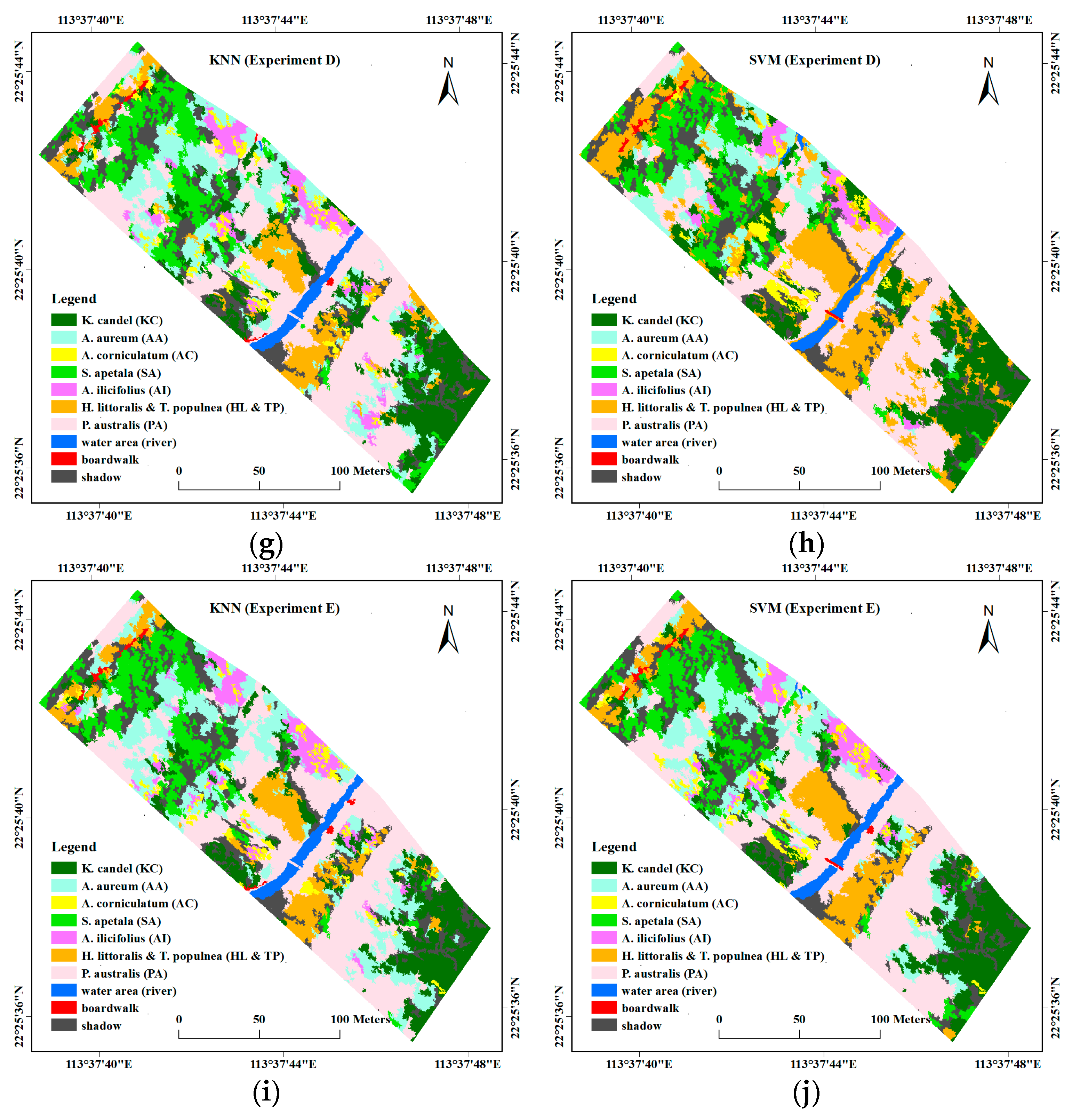
4.2. Comparison of Object-Based Classification Results

To evaluate the performance of different feature combinations, five schemes were carried out in this study using the KNN and SVM classifiers.

• Experiment A: spectral features, using 32 selected spectral bands (mean values) selected from the CART method, including band 1–2, band 8–10, band 14, band 17–19, band 23–24, band 26, band 28–29, band 48, band 52, band 56–57, band 62–64, band 68–70, band 72, band 75, band 79–80, band 82–83, band 91, and band 107, brightness and max.diff.
• Experiment B: stacking spectral features in Experiment A, hyperspectral VIs, and textural features.
• Experiment C: stacking spectral features in Experiment A and height information.
• Experiment D: stacking all the features together, including spectral features in Experiment A, hyperspectral VIs, textural features, and height information.
• Experiment E: 14 features selected from Experiment D using CFS, including four spectral bands, i.e., band 10, band 23, band 62 and band 91, four hyperspectral VIs, i.e., NDVI, TCARI, MCARI2, and PRI, five textural features, i.e., ASM (band 50), COR (band 8 and 25), MEAN (band 8), and StdDev (band 8), and UAV-derived DSM.

Figure 7 presents the classification results for the five feature combinations produced from the KNN and SVM object-based classification. Both of the classifiers performed well in terms of the spatial distribution of different mangrove species in the study site. According to visual judgment and based on several field investigations, the SVM classifier provided better performance. From visual comparison of the classification maps, two dominated mangrove stands, i.e., KC and SA, showed a clearly zonal distribution, as well as HL and TP. When compared with KNN, these three mangrove stands were rarely classified as other stands or land-cover types. Parts of the accompanying PA standing along the edge of the river were mistakenly classified as boardwalks in most of the KNN results, whereas this phenomenon rarely occurred in the SVM results. Moreover, by incorporating height information, mangrove stands, or other land covers with significant height differences, such as SA, AA, and PA could be well distinguished.

Table 6. Summary of classification accuracies of the different classification schemes using KNN.

Classified Category	Experiment A		Experiment B		Experiment C		Experiment D		Experiment E
	PA	UA	PA	UA	PA	UA	PA	UA	PA	UA
K. candel (KC)	81.03	69.12	77.59	70.31	79.31	76.67	79.31	73.02	93.55	67.44
A. aureum (AA)	80.65	49.02	87.10	65.85	100	51.67	90.32	73.68	59.09	72.22
A. corniculatum (AC)	40.00	75.00	60.00	90.00	46.67	84.00	60.00	93.10	97.50	72.22
S. apetala (SA)	80.49	76.74	90.24	86.05	80.49	94.29	90.24	88.10	50.00	100
A. ilicifolius (AI)	50.00	44.00	59.09	76.47	50.00	57.89	77.27	80.95	84.48	87.50
H. littoralis & T. populnea (HL & TP)	63.41	92.86	87.80	85.71	75.61	88.57	90.24	86.05	93.10	87.10
P. australis (PA)	92.50	75.51	92.50	74.00	97.50	73.58	95.00	74.51	57.78	81.25
water area (river)	77.78	77.78	77.78	100	77.78	77.78	77.78	100	77.78	100
boardwalk	10.00	100	50.00	100	20.00	100	50.00	100	90.24	92.50
shadow	93.10	96.43	89.66	89.66	93.10	96.43	89.66	89.66	85.37	83.33
OA (%)	71.34		79.70		76.12		82.09		81.79
Kappa	0.675		0.770		0.730		0.797		0.774

and

Table 7. Summary of classification accuracies of the different classification schemes using SVM.

Classified Category	Experiment A		Experiment B		Experiment C		Experiment D		Experiment E
	PA	UA	PA	UA	PA	UA	PA	UA	PA	UA
K. candel (KC)	81.03	70.15	93.10	79.41	81.03	79.66	91.38	81.54	93.55	85.29
A. aureum (AA)	74.19	79.31	83.87	81.25	96.77	68.18	83.87	96.30	68.18	88.24
A. corniculatum (AC)	55.56	71.43	77.78	92.11	64.44	76.32	75.56	91.89	100	78.43
S. apetala (SA)	82.93	79.07	87.80	92.31	78.05	94.12	90.24	94.87	100	100
A. ilicifolius (AI)	45.45	66.67	63.64	93.33	50.00	61.11	72.73	88.89	93.10	90.00
H. littoralis & T. populnea (HL & TP)	85.37	74.47	90.24	86.05	92.68	97.44	92.68	76.00	100	90.63
P. australis (PA)	92.50	80.43	100	90.91	100	80.00	97.50	92.86	77.78	89.74
water area (river)	77.78	100	88.89	100	77.78	100	88.89	100	72.22	100
boardwalk	70.00	100	100	100	70.00	100	100	100	90.24	94.87
shadow	96.55	87.50	93.10	90.00	96.55	87.50	96.55	90.32	92.68	95.00
OA (%)	77.61		88.06		82.39		88.66		89.55
Kappa	0.746		0.864		0.801		0.871		0.882

summarize the classification accuracy assessment results. These results show that the SVM classifier outperformed the KNN classifier. The SVM object-based classification gave the best performance with an overall classification accuracy of 89.55% and a kappa coefficient of 0.882, and the classification accuracies for most of the mangrove species were greater than 80% in terms of PA and UA. For example, when compared to KNN, the SVM classifier reduced the miss-classification (the class in consideration being identified as another class) or misclassification (another class being identified as the class in consideration) of mangrove species KC and SA, as evidenced by higher values of PA and UA. Furthermore, in a more detailed comparison, both classifiers gave low values of PA and UA for the undergrowth AI stands, as a result of interference from the neighboring taller mangrove stands.

For the scheme in Experiment D, both the KNN and SVM classification results outperformed three combination schemes, i.e., Experiment A, B and C. Moreover, a comparison between Experiments A and C, or between Experiments B and D, shows that height information played an important role in improving classification accuracy. For example, the accuracy increments of taller plants, including SA, HL, and TP, were greater than those for undergrowth plants, such as AC and AI. The AC stands had high omission error with a low value of producer’s accuracy in this study site and were often placed into other classes, i.e., KC, AA, and AI, due to similarities in color and small height differences. This example demonstrates that height information can complement spectral features to enhance classification accuracy. For Experiment E, based on 14 features selected by CFS, the classification accuracy of the KNN classifier was close to that of using all 67 features, while the SVM classifier obtained higher classification accuracy. These results are consistent with previous studies [93,94] that feature selection of the high-dimensional classification, for example, plethora of spectral bands or object features, can improve the performance and efficiency by eliminating redundant information.

The UAV hyperspectral image provides more spectral and spatial details, which improves classification accuracy, whereas the UAV-derived DSM data provide spatial and structural information that increase the capability to separate different mangrove species. For instance, Jia et al. [20] combined Hyperion data and SPOT-5 data to distinguish four mangrove species, but this study used the UAV hyperspectral image with both narrower bandwidths and higher spatial resolution and could identify more mangrove species. Without regard to differences among study sites, the classification accuracies reported here were higher than those of Kamal and Phinn [21], who used CASI-2 data for three mangrove species mapping, especially when incorporating height information into the classification features. These results are also consistent with the results of work by Liu and Bo [57], who concluded that height information in object-based crop species classification could improve classification accuracy.

5. Conclusions

In this study, object-based mangrove species classification was carried out using the UAV hyperspectral image from the UHD 185 hyperspectral sensor and UAV-derived DSM data on Qi’ao Island. To evaluate the effectiveness of the UAV hyperspectral image, comparisons of different object-based classifiers were performed. In addition, the contributions of the spectral and textural features of the UAV hyperspectral image, and of the height information obtained from the UAV-derived DSM data, to the separability of mangrove species were studied.

This paper has contrasted the performance of different feature combinations for mangrove species object-based classification. Based on qualitative and quantitative analysis of these experiments, the following conclusions could be drawn. (1) When compared with KNN, the SVM classifier proved to be more accurate for mangrove species classification by stacking all the features together, with an overall accuracy of 88.66% and a kappa coefficient of 0.871. Feature reduction can further improve the classification accuracies and performances of SVM. (2) The combination of spectral features (including VIs) and spatial features (i.e., textural features and height information) provided higher accuracy of mangrove species classification. In particular, the height information was effective for separating the mangrove species with similar spectral signatures, but different mean heights. Experimental results verify the effectiveness of the framework presented here using the UAV hyperspectral image in mangrove species classification.

References

1. Peng, L. A review on the mangrove research in China. J. Xiamen Univ. Nat. Sci. 2001, 40, 592–603. [Google Scholar]
2. Bahuguna, A.; Nayak, S.; Roy, D. Impact of the tsunami and earthquake of 26th December 2004 on the vital coastal ecosystems of the Andaman and Nicobar Islands assessed using RESOURCESAT AWIFS data. Int. J. Appl. Earth Obs. Geoinf. 2008, 10, 229–237. [Google Scholar] [CrossRef]
3. Food and Agriculture Organization (FAO). The World’s Mangroves 1980–2005; FAO: Rome, Italy, 2007. [Google Scholar]
4. Li, W.; Niu, Z.; Chen, H.; Li, D.; Wu, M.; Zhao, W. Remote estimation of canopy height and aboveground biomass of maize using high-resolution stereo images from a low-cost unmanned aerial vehicle system. Ecol. Indic. 2016, 67, 637–648. [Google Scholar] [CrossRef]
5. Giri, C.; Ochieng, E.; Tieszen, L.L.; Zhu, Z.; Singh, A.; Loveland, T.; Masek, J.; Duke, N. Status and distribution of mangrove forests of the world using earth observation satellite data. Glob. Ecol. Biogeogr. 2011, 20, 154–159. [Google Scholar] [CrossRef]
6. Green, E.P.; Clark, C.D.; Mumby, P.J.; Edwards, A.J.; Ellis, A. Remote sensing techniques for mangrove mapping. Int. J. Remote Sens. 1998, 19, 935–956. [Google Scholar] [CrossRef]
7. Held, A.; Ticehurst, C.; Lymburner, L.; Williams, N. High resolution mapping of tropical mangrove ecosystems using hyperspectral and radar remote sensing. Int. J. Remote Sens. 2003, 24, 2739–2759. [Google Scholar] [CrossRef]
8. Giri, S.; Mukhopadhyay, A.; Hazra, S.; Mukherjee, S.; Roy, D.; Ghosh, S.; Ghosh, T.; Mitra, D. A study on abundance and distribution of mangrove species in Indian Sundarban using remote sensing technique. J. Coast. Conserv. 2014, 18, 359–367. [Google Scholar] [CrossRef]
9. Liu, K.; Liu, L.; Liu, H.; Li, X.; Wang, S. Exploring the effects of biophysical parameters on the spatial pattern of rare cold damage to mangrove forests. Remote Sens. Environ. 2014, 150, 20–33. [Google Scholar] [CrossRef]
10. Wang, L.; Silváncárdenas, J.L.; Sousa, W.P. Neural network classification of mangrove species from multi-seasonal IKONOS imagery. Photogramm. Eng. Remote Sens. 2008, 74, 921–927. [Google Scholar] [CrossRef]
11. Neukermans, G.; Dahdouh-Guebas, F.; Kairo, J.G.; Koedam, N. Mangrove species and stand mapping in gazi bay (Kenya) using quickbird satellite imagery. J. Spat. Sci. 2008, 53, 75–86. [Google Scholar] [CrossRef]
12. Wang, L.; Sousa, W.P.; Peng, G.; Biging, G.S. Comparison of IKONOS and quickbird images for mapping mangrove species on the caribbean coast of panama. Remote Sens. Environ. 2004, 91, 432–440. [Google Scholar] [CrossRef]
13. Zhu, Y.; Liu, K.; Liu, L.; Wang, S.; Liu, H. Retrieval of mangrove aboveground biomass at the individual species level with worldview-2 images. Remote Sens. 2015, 7, 12192–12214. [Google Scholar] [CrossRef]
14. Tang, H.; Liu, K.; Zhu, Y.; Wang, S.; Liu, L.; Song, S. Mangrove community classification based on worldview-2 image and SVM method. Acta Sci. Nat. Univ. Sunyatseni 2015, 54, 102–111. [Google Scholar]
15. Pu, R. Mapping urban forest tree species using IKONOS imagery: Preliminary results. Environ. Monit. Assess. 2011, 172, 199–214. [Google Scholar] [CrossRef] [PubMed]
16. Tong, Q.; Zhang, B.; Zheng, L. Hyperspectral Remote Sensing: Principles, Techniques and Applications; Higher Education Press: Beijing, China, 2006. [Google Scholar]
17. Guo, M.; Li, J.; Sheng, C.; Xu, J.; Wu, L. A review of wetland remote sensing. Sensors 2017, 17. [Google Scholar] [CrossRef] [PubMed]
18. Hirano, A.; Madden, M.; Welch, R. Hyperspectral image data for mapping wetland vegetation. Wetlands 2003, 23, 436–448. [Google Scholar] [CrossRef]
19. Koedsin, W.; Vaiphasa, C. Discrimination of tropical mangroves at the species level with EO-1 hyperion data. Remote Sens. 2013, 5, 3562–3582. [Google Scholar] [CrossRef]
20. Jia, M.; Zhang, Y.; Wang, Z.; Song, K.; Ren, C. Mapping the distribution of mangrove species in the Core Zone of Mai Po Marshes Nature Reserve, Hong Kong, using hyperspectral data and high-resolution data. Int. J. Appl. Earth Obs. Geoinf. 2014, 33, 226–231. [Google Scholar] [CrossRef]
21. Kamal, M.; Phinn, S. Hyperspectral data for mangrove species mapping: A comparison of pixel-based and object-based approach. Remote Sens. 2011, 3, 2222–2242. [Google Scholar] [CrossRef]
22. Fauvel, M.; Tarabalka, Y.; Benediktsson, J.A.; Chanussot, J.; Tilton, J.C. Advances in spectral-spatial classification of hyperspectral images. Proc. IEEE 2013, 101, 652–675. [Google Scholar] [CrossRef]
23. Matsuki, T.; Yokoya, N.; Iwasaki, A. Hyperspectral tree species classification of Japanese complex mixed forest with the aid of LiDAR data. IEEE J. Sel. Top. Appl. Earth Obs. Remote Sens. 2015, 8, 2177–2187. [Google Scholar] [CrossRef]
24. Balas, C.; Pappas, C.; Epitropou, G. Multi/Hyper-Spectral Imaging. In Handbook of Biomedical Optics; Boas, D.A., Pitris, C., Ramanujam, N., Eds.; CRC Press: Boca Raton, FL, USA, 2011. [Google Scholar]
25. Colomina, I.; Molina, P. Unmanned aerial systems for photogrammetry and remote sensing: A review. ISPRS J. Photogramm. Remote Sens. 2014, 92, 79–97. [Google Scholar] [CrossRef]
26. Aasen, H.; Burkart, A.; Bolten, A.; Bareth, G. Generating 3D hyperspectral information with lightweight UAV snapshot cameras for vegetation monitoring: From camera calibration to quality assurance. ISPRS J. Photogramm. Remote Sens. 2015, 108, 245–259. [Google Scholar] [CrossRef]
27. Bareth, G.; Aasen, H.; Bendig, J.; Gnyp, M.L.; Bolten, A.; Jung, A.; Michels, R.; Soukkamäki, J. Low-weight and UAV-based hyperspectral full-frame cameras for monitoring crops: Spectral comparison with portable spectroradiometer measurements. Photogramm. Fernerkund. Geoinf. 2015, 2015, 69–79. [Google Scholar] [CrossRef]
28. Cui, J.; Zhang, S.; Zhang, J.; Liu, X.; Ding, R.; Liu, H. Determining surface magnetic susceptibility of loess-paleosol sections based on spectral features: Application to a UHD 185 hyperspectral image. Int. J. Appl. Earth Obs. Geoinf. 2016, 50, 159–169. [Google Scholar] [CrossRef]
29. Hruska, R.; Mitchell, J.; Anderson, M.; Glenn, N.F. Radiometric and geometric analysis of hyperspectral imagery acquired from an unmanned aerial vehicle. Remote Sens. 2012, 4, 2736–2752. [Google Scholar] [CrossRef]
30. Mitchell, J.J.; Glenn, N.F.; Anderson, M.O.; Hruska, R.C.; Halford, A.; Baun, C.; Nydegger, N. Unmanned aerial vehicle (UAV) hyperspectral remote sensing for dryland vegetation monitoring. In Proceedings of the Workshop on Hyperspectral Image & Signal Processing: Evolution in Remote Sensing, Shanghai, China, 4–7 June 2012; pp. 1–10. [Google Scholar]
31. Zarco-Tejada, P.J.; González-Dugo, V.; Berni, J.A.J. Fluorescence, temperature and narrow-band indices acquired from a UAV platform for water stress detection using a micro-hyperspectral imager and a thermal camera. Remote Sens. Environ. 2012, 117, 322–337. [Google Scholar] [CrossRef]
32. Zarco-Tejada, P.J.; Catalina, A.; González, M.R.; Martín, P. Relationships between net photosynthesis and steady-state chlorophyll fluorescence retrieved from airborne hyperspectral imagery. Remote Sens. Environ. 2013, 136, 247–258. [Google Scholar] [CrossRef]
33. Zarcotejada, P.J.; Guilléncliment, M.L.; Hernándezclemente, R.; Catalina, A.; González, M.R.; Martín, P. Estimating leaf carotenoid content in vineyards using high resolution hyperspectral imagery acquired from an unmanned aerial vehicle (UAV). Agric. For. Meteorol. 2013, 171, 281–294. [Google Scholar] [CrossRef]
34. Zarco-Tejada, P.J.; Morales, A.; Testi, L.; Villalobos, F.J. Spatio-temporal patterns of chlorophyll fluorescence and physiological and structural indices acquired from hyperspectral imagery as compared with carbon fluxes measured with eddy covariance. Remote Sens. Environ. 2013, 133, 102–115. [Google Scholar] [CrossRef]
35. Calderón, R.; Navas-Cortés, J.A.; Lucena, C.; Zarco-Tejada, P.J. High-resolution airborne hyperspectral and thermal imagery for early detection of verticillium wilt of olive using fluorescence, temperature and narrow-band spectral indices. Remote Sens. Environ. 2013, 139, 231–245. [Google Scholar] [CrossRef]
36. Yuan, H.; Yang, G.; Li, C.; Wang, Y.; Liu, J.; Yu, H.; Feng, H.; Xu, B.; Zhao, X.; Yang, X. Retrieving soybean leaf area index from unmanned aerial vehicle hyperspectral remote sensing: Analysis of RF, ANN, and SVM regression models. Remote Sens. 2017, 9. [Google Scholar] [CrossRef]
37. Lu, G.; Yang, G.; Zhao, X.; Wang, Y.; Li, C.; Zhang, X. Inversion of soybean fresh biomass based on multi-payload unmanned aerial vehicles (UAVs). Soybean Sci. 2017, 36, 41–50. [Google Scholar]
38. Zhao, X.; Yang, G.; Liu, J.; Zhang, X.; Xu, B.; Wang, Y.; Zhao, C.; Gai, J. Estimation of soybean breeding yield based on optimization of spatial scale of UAV hyperspectral image. Trans. Chin. Soc. Agric. Eng. 2017, 33, 110–116. [Google Scholar]
39. Gao, L.; Yang, G.; Yu, H.; Xu, B.; Zhao, X.; Dong, J.; Ma, Y. Retrieving winter wheat leaf area index based on unmanned aerial vehicle hyperspectral remote sensing. Trans. Chin. Soc. Agric. Eng. 2016, 32, 113–120. [Google Scholar]
40. Qin, Z.; Chang, Q.; Xie, B.; Jian, S. Rice leaf nitrogen content estimation based on hysperspectral imagery of UAV in yellow river diversion irrigation district. Trans. Chin. Soc. Agric. Eng. 2016, 32, 77–85. [Google Scholar]
41. Tian, M.; Ban, S.; Chang, Q.; You, M.; Dan, L.; Li, W.; Wang, S. Use of hyperspectral images from UAV-based imaging spectroradiometer to estimate cotton leaf area index. Trans. Chin. Soc. Agric. Eng. 2016, 32, 102–108. [Google Scholar]
42. Yue, J.; Yang, G.; Li, C.; Li, Z.; Wang, Y.; Feng, H.; Xu, B. Estimation of winter wheat above-ground biomass using unmanned aerial vehicle-based snapshot hyperspectral sensor and crop height improved models. Remote Sens. 2017, 9. [Google Scholar] [CrossRef]
43. Sankey, T.; Donager, J.; McVay, J.; Sankey, J.B. UAV LiDAR and hyperspectral fusion for forest monitoring in the southwestern USA. Remote Sens. Environ. 2017, 195, 30–43. [Google Scholar] [CrossRef]
44. Li, Q.S.; Wong, F.K.K.; Fung, T. Assessing the utility of UAV-borne hyperspectral image and photogrammetry derived 3D data for wetland species distribution quick mapping. ISPRS Int. Arch. Photogramm. Remote Sens. Spat. Inf. Sci. 2017, XLII-2/W6, 209–215. [Google Scholar] [CrossRef]
45. D’iorio, M.; Jupiter, S.D.; Cochran, S.A.; Potts, D.C. Optimizing remote sensing and GIS tools for mapping and managing the distribution of an invasive mangrove (Rhizophora mangle) on South Molokai, Hawaii. Mar. Geodesy 2007, 30, 125–144. [Google Scholar] [CrossRef]
46. Yang, C.; Everitt, J.H.; Fletcher, R.S.; Jensen, R.R.; Mausel, P.W. Evaluating aisa + hyperspectral imagery for mapping black mangrove along the south texas gulf coast. Photogramm. Eng. Remote Sens. 2009, 75, 425–435. [Google Scholar] [CrossRef]
47. Chakravortty, S. Analysis of end member detection and subpixel classification algorithms on hyperspectral imagery for tropical mangrove species discrimination in the Sunderbans Delta, India. J. Appl. Remote Sens. 2013, 7. [Google Scholar] [CrossRef]
48. Chakravortty, S.; Shah, E.; Chowdhury, A.S. Application of spectral unmixing algorithm on hyperspectral data for mangrove species classification. In Proceedings of the International Conference on Applied Algorithms, Kolkata, India, 13–15 January 2014; Springer: New York, NY, USA, 2014; pp. 223–236. [Google Scholar]
49. Chakravortty, S.; Sinha, D. Analysis of multiple scattering of radiation amongst end members in a mixed pixel of hyperspectral data for identification of mangrove species in a mixed stand. J. Indian Soc. Remote Sens. 2015, 43, 559–569. [Google Scholar] [CrossRef]
50. Zhang, Z.; Kazakova, A.; Moskal, L.; Styers, D. Object-based tree species classification in urban ecosystems using LiDAR and hyperspectral data. Forests 2016, 7. [Google Scholar] [CrossRef]
51. Kumar, T.; Panigrahy, S.; Kumar, P.; Parihar, J.S. Classification of floristic composition of mangrove forests using hyperspectral data: Case study of Bhitarkanika National Park, India. J. Coast. Conserv. 2013, 17, 121–132. [Google Scholar] [CrossRef]
52. Wong, F.K.; Fung, T. Combining EO-1 hyperion and ENVISAT ASAR data for mangrove species classification in Mai Po Ramsar Site, Hong Kong. Int. J. Remote Sens. 2014, 35, 7828–7856. [Google Scholar] [CrossRef]
53. Duro, D.C.; Franklin, S.E.; Dubé, M.G. A comparison of pixel-based and object-based image analysis with selected machine learning algorithms for the classification of agricultural landscapes using spot-5 HRG imagery. Remote Sens. Environ. 2012, 118, 259–272. [Google Scholar] [CrossRef]
54. Pu, R. Tree species classification. In Remote Sensing of Natural Resources; CRC Press: Boca Raton, FL, USA, 2013; pp. 239–258. [Google Scholar]
55. Li, S.S.; Tian, Q.J. Mangrove canopy species discrimination based on spectral features of geoeye-1 imagery. Spectrosc. Spectr. Anal. 2013, 33, 136–141. [Google Scholar]
56. Xiao, H.Y.; Zeng, H.; Zan, Q.J.; Bai, Y.; Cheng, H.H. Decision tree model in extraction of mangrove community information using hyperspectral image data. J. Remote Sens. 2007, 11, 531–537. [Google Scholar]
57. Liu, X.; Bo, Y. Object-based crop species classification based on the combination of airborne hyperspectral images and LiDAR data. Remote Sens. 2015, 7, 922–950. [Google Scholar] [CrossRef]
58. Chadwick, J. Integrated LiDAR and IKONOS multispectral imagery for mapping mangrove distribution and physical properties. Int. J. Remote Sens. 2011, 32, 6765–6781. [Google Scholar] [CrossRef]
59. Kamal, M.; Phinn, S.; Johansen, K. Object-based approach for multi-scale mangrove composition mapping using multi-resolution image datasets. Remote Sens. 2015, 7, 4753–4783. [Google Scholar] [CrossRef]
60. Zarco-Tejada, P.J.; Diaz-Varela, R.; Angileri, V.; Loudjani, P. Tree height quantification using very high resolution imagery acquired from an unmanned aerial vehicle (UAV) and automatic 3D photo-reconstruction methods. Eur. J. Agron. 2014, 55, 89–99. [Google Scholar] [CrossRef]
61. Turner, D.; Lucieer, A.; Wallace, L. Direct georeferencing of ultrahigh-resolution UAV imagery. IEEE Trans. Geosci. Remote Sens. 2014, 52, 2738–2745. [Google Scholar] [CrossRef]
62. Liao, B.W.; Wei, G.; Zhang, J.E.; Tang, G.L.; Lei, Z.S.; Yang, X.B. Studies on dynamic development of mangrove communities on Qi’ao Island, Zhuhai. J. South China Agric. Univ. 2008, 29, 59–64. [Google Scholar]
63. Liu, B.E.; Liao, B.W. Mangrove reform-planting trial on Qi’ao Island. Ecol. Sci. 2013, 32, 534–539. [Google Scholar]
64. Baatz, M.; Schäpe, A. Multiresolution Segmentation: An Optimization Approach for High Quality Multi-Scale Image Segmentation. Available online: http://www.ecognition.com/sites/default/files/405_baatz_fp_12.pdf (accessed on 21 November 2017).
65. Cheng, J.; Bo, Y.; Zhu, Y.; Ji, X. A novel method for assessing the segmentation quality of high-spatial resolution remote-sensing images. Int. J. Remote Sens. 2014, 35, 3816–3839. [Google Scholar] [CrossRef]
66. Benz, U.C.; Hofmann, P.; Willhauck, G.; Lingenfelder, I.; Heynen, M. Multi-resolution, object-oriented fuzzy analysis of remote sensing data for GIS-ready information. ISPRS J. Photogramm. Remote Sens. 2004, 58, 239–258. [Google Scholar] [CrossRef]
67. Qian, Y.; Zhou, W.; Yan, J.; Li, W.; Han, L. Comparing machine learning classifiers for object-based land cover classification using very high resolution imagery. Remote Sens. 2014, 7, 153–168. [Google Scholar] [CrossRef]
68. Haboudane, D.; Miller, J.R.; Tremblay, N.; Zarco-Tejada, P.J.; Dextraze, L. Integrated narrow-band vegetation indices for prediction of crop chlorophyll content for application to precision agriculture. Remote Sens. Environ. 2002, 81, 416–426. [Google Scholar] [CrossRef]
69. Rondeaux, G.; Steven, M.; Baret, F. Optimization of soil-adjusted vegetation indices. Remote Sens. Environ. 1996, 55, 95–107. [Google Scholar] [CrossRef]
70. Zarco-Tejada, P.J.; Berjón, A.; López-Lozano, R.; Miller, J.R.; Martín, P.; Cachorro, V.; González, M.; De Frutos, A. Assessing vineyard condition with hyperspectral indices: Leaf and canopy reflectance simulation in a row-structured discontinuous canopy. Remote Sens. Environ. 2005, 99, 271–287. [Google Scholar] [CrossRef]
71. Hernández-Clemente, R.; Navarro-Cerrillo, R.M.; Suárez, L.; Morales, F.; Zarco-Tejada, P.J. Assessing structural effects on PRI for stress detection in conifer forests. Remote Sens. Environ. 2011, 115, 2360–2375. [Google Scholar] [CrossRef]
72. Rouse, J.W.; Haas, R.H.; Schell, J.A.; Deering, D.W. Monitoring Vegetation Systems in the Great Plains with ERTS; Paper-A20; National Aeronautics and Space Administration (NASA): Washington, DC, USA, 1974; pp. 309–317.
73. Roujean, J.-L.; Breon, F.-M. Estimating par absorbed by vegetation from bidirectional reflectance measurements. Remote Sens. Environ. 1995, 51, 375–384. [Google Scholar] [CrossRef]
74. Haboudane, D.; Miller, J.R.; Pattey, E.; Zarco-Tejada, P.J.; Strachan, I.B. Hyperspectral vegetation indices and novel algorithms for predicting green LAI of crop canopies: Modeling and validation in the context of precision agriculture. Remote Sens. Environ. 2004, 90, 337–352. [Google Scholar] [CrossRef]
75. Haralick, R.M.; Shanmugam, K. Textural features for image classification. IEEE Trans. Syst. Man Cybern. 1973, 6, 610–621. [Google Scholar] [CrossRef]
76. Tan, Y.; Xia, W.; Xu, B.; Bai, L. Multi-feature classification approach for high spatial resolution hyperspectral images. J. Indian Soc. Remote Sens. 2017, 1–9. [Google Scholar] [CrossRef]
77. Pu, R.; Gong, P. Hyperspectral remote sensing of vegetation bioparameters. In Advances in Environmental Remote Sensing: Sensors, Algorithm, and Applications; CRC Press: Boca Raton, FL, USA, 2011; pp. 101–142. [Google Scholar]
78. Breiman, L.; Friedman, J.; Olshen, R.; Stone, C. Classification and Regresssion Trees; Wadsworth International Group: Belmont, CA, USA, 1984. [Google Scholar]
79. Gomez-Chova, L.; Calpe, J.; Soria, E.; Camps-Valls, G.; Martin, J.D.; Moreno, J. CART-based feature selection of hyperspectral images for crop cover classification. In Proceedings of the International Conference on Image Processing, Barcelona, Spain, 14–17 September 2003; pp. 589–592. [Google Scholar]
80. Bittencourt, H.R.; Clarke, R.T. Feature selection by using classification and regression trees (CART). Int. Arch. Photogramm. Remote Sens. Spat. Inf. Sci. 2004, 35, 66–70. [Google Scholar]
81. Hall, M.A. Feature selection for discrete and numeric class machine learning. In Proceedings of the Seventeenth International Conference on Machine Learning, Stanford, CA, USA, 29 June–2 July 2000; pp. 359–366. [Google Scholar]
82. Wollmer, M.; Schuller, B.; Eyben, F.; Rigoll, G. Combining long short-term memory and dynamic bayesian networks for incremental emotion-sensitive artificial listening. IEEE J. Sel. Top. Signal Process. 2010, 4, 867–881. [Google Scholar] [CrossRef]
83. Hall, M.A.; Holmes, G. Benchmarking attribute selection techniques for discrete class data mining. IEEE Trans. Knowl. Data Eng. 2003, 15, 1437–1447. [Google Scholar] [CrossRef]
84. Piedra-Fernandez, J.A.; Canton-Garbin, M.; Wang, J.Z. Feature selection in avhrr ocean satellite images by means of filter methods. IEEE Trans. Geosci. Remote Sens. 2010, 48, 4193–4203. [Google Scholar] [CrossRef]
85. Aguirre-Gutiérrez, J.; Seijmonsbergen, A.C.; Duivenvoorden, J.F. Optimizing land cover classification accuracy for change detection, a combined pixel-based and object-based approach in a mountainous area in mexico. Appl. Geogr. 2012, 34, 29–37. [Google Scholar] [CrossRef]
86. Cover, T.; Hart, P. Nearest neighbor pattern classification. IEEE Trans. Inf. Theory 1967, 13, 21–27. [Google Scholar] [CrossRef]
87. Hart, B.P.E. The condensed nearest neighbor rule. IEEE Trans. Inf. Theory 1968, 14, 515–516. [Google Scholar] [CrossRef]
88. Yang, J.M.; Yu, P.T.; Kuo, B.C. A nonparametric feature extraction and its application to nearest neighbor classification for hyperspectral image data. IEEE Trans. Geosci. Remote Sens. 2010, 48, 1279–1293. [Google Scholar] [CrossRef]
89. Féret, J.B.; Asner, G.P. Semi-supervised methods to identify individual crowns of lowland tropical canopy species using imaging spectroscopy and LiDAR. Remote Sens. 2012, 4, 2457–2476. [Google Scholar] [CrossRef]
90. Mountrakis, G.; Im, J.; Ogole, C. Support vector machines in remote sensing: A review. ISPRS J. Photogramm. Remote Sens. 2011, 66, 247–259. [Google Scholar] [CrossRef]
91. Chang, C.C.; Lin, C.J. LIBSVM: A library for support vector machines. ACM Trans. Intell. Syst. Technol. 2011, 2, 27. [Google Scholar] [CrossRef]
92. Congalton, R.G.; Green, K. Assessing the Accuracy of Remotely Sensed Data: Principles and Practices; CRC Press: Boca Raton, FL, USA, 2008. [Google Scholar]
93. Ma, L.; Cheng, L.; Li, M.; Liu, Y.; Ma, X. Training set size, scale, and features in geographic object-based image analysis of very high resolution unmanned aerial vehicle imagery. ISPRS J. Photogramm. Remote Sens. 2015, 102, 14–27. [Google Scholar] [CrossRef]
94. Gomez-Chova, L.; Calpe, J.; Camps-Valls, G.; Martin, J.D.; Soria, E.; Vila, J.; Alonso-Chorda, L.; Moreno, J. Feature selection of hyperspectral data through local correlation and SFFS for crop classification. In Proceedings of the 2003 IEEE International Geoscience & Remote Sensing Symposium, Toulouse, France, 21–25 July 2003; pp. 555–557. [Google Scholar]
Figure 1. Location of the study area (Qi’ao Island), showing the WorldView-2 image (lower left) (false color composite (FCC) composed of R, band 7; G, band 5; B, band 3); and the UHD 185 hyperspectral image (right) covering the study site on Qi’ao Island (true color composition of R, band 50, G, band 25, and B, band 8). The blue polygon shows the boundary of the mangrove area on Qi’ao Island, and the yellow polygon shows the extent of the study site.
Remotesensing 10 00089 g001
Figure 2. Carrier platform multi-rotor unmanned aerial vehicles (UAV) and image capture system with UHD 185 hyperspectral sensor.
Remotesensing 10 00089 g002
Figure 3. Mean spectral reflectance profiles of six mangrove species extracted from a UAV hyperspectral image within the study site.
Remotesensing 10 00089 g003
Figure 4. Three-dimensional (3D) view of UAV-derived digital surface model (DSM) (a) and mean heights of six mangrove species calculated from DSM (b).
Remotesensing 10 00089 g004
Figure 5. Flowchart for object-based mangrove species classification based on UAV hyperspectral image.
Remotesensing 10 00089 g005
Figure 6. Local representation of image segmentation using different scale factors, shape indices, and compactness parameters. (a) image segmentation results with different scales (shape index = 0.1, compactness = 0.5), (b) image segmentation results with different shape indices (scale = 100, compactness = 0.5), (c) image segmentation results with different compactness values (scale = 100, shape index = 0.5).
Remotesensing 10 00089 g006aRemotesensing 10 00089 g006b
Figure 7. Classification maps of different feature combinations with different classifiers. (a) Experiment A using k-nearest neighbor (KNN); (b) Experiment A using support vector machine (SVM); (c) Experiment B using KNN; (d) Experiment B using SVM; (e) Experiment C using KNN; (f) Experiment C using SVM; (g) Experiment D using KNN; (h) Experiment D using SVM; (i) Experiment E using KNN; (j) Experiment E using SVM.
Remotesensing 10 00089 g007aRemotesensing 10 00089 g007b