Analysis of the Spatial Variability of Land Surface Variables for ET Estimation: Case Study in HiWATER Campaign
by
 , ,
, ,
Xiaojun Li
1,2,3 ,
,
Xiaozhou Xin
1,2,*,
Zhiqing Peng
1,3,
Hailong Zhang
1,2,
Chuanxiang Yi
4 and
Bin Li
5 1
State Key Laboratory of Remote Sensing Science, Jointly Sponsored by Institute of Remote Sensing and Digital Earth of Chinese Academy of Sciences and Beijing Normal University, Beijing 100101, China
2
Joint Center for Global Change Studies (JCGCS), Beijing 100875, China
3
University of Chinese Academy of Sciences, Beijing 100049, China
4
College of Applied Meteorology, Nanjing University of Information Science & Technology, Nanjing 210044, China
5
Inner Mongolia Ecological and Agricultural Meteorological Center, Hohhot 010051, China
*
Author to whom correspondence should be addressed.
Remote Sens. 2018, 10(1), 91; https://doi.org/10.3390/rs10010091
Submission received: 13 December 2017
/
Revised: 8 January 2018
/
Accepted: 10 January 2018
/
Published: 11 January 2018
(This article belongs to the Special Issue Advances in Quantitative Remote Sensing in China – In Memory of Prof. Xiaowen Li)
Abstract
:Heterogeneity, including the inhomogeneity of landscapes and surface variables, significantly affects the accuracy of evapotranspiration (ET) (or latent heat flux, LE) estimated from remote sensing satellite data. However, most of the current research uses statistical methods in the mixed pixel to correct the ET or LE estimation error, and there is a lack of research from the perspective of the remote sensing model. The method of using frequency distributions or generalized probability density functions (PDFs), which is called the “statistical-dynamical” approach to describe the heterogeneity of land surface characteristics, is a good way to solve the problem. However, in attempting to produce an efficient PDF-based parameterization of remotely sensed ET or LE, first and foremost, it is necessary to systematically understand the variables that are most consistent with the heterogeneity (i.e., variability for a fixed target area or landscape, where the variation in the surface parameter value is primarily concerned with the PDF-based model) of surface turbulence flux. However, the use of PDF alone does not facilitate direct comparisons of the spatial variability of surface variables. To address this issue, the objective of this study is to find an indicator based on PDF to express variability of surface variables. We select the dimensionless or dimensional consistent coefficient of variation (CV), Gini coefficient and entropy to express variability. Based on the analysis of simulated data and field experimental data, we find that entropy is more stable and accurate than the CV and Gini coefficient for expressing the variability of surface variables. In addition, the results of the three methods show that the variability of the leaf area index (LAI) is greater than that of the land surface temperature (LST). Our results provide a suitable method for comparing the variability of different variables.
1. Introduction
Evapotranspiration plays a key role in the Earth’s surface energy and water balances, and it has substantial effects on global climate change, water management and crop yield [1,2,3]. Satellite-based remote sensing has been identified as a suitable means of mapping the spatial distribution of ET or LE. Because of technical and methodological limitations, many remote sensing-based ET or LE models have been conducted under quite homogeneous and flat conditions, with the use of decametric to kilometric spatial resolution sensors [4,5]. However, the Earth’s surface geometry, physical processes and associated variables are inherently heterogeneous. Due to the nonlinear nature of many land surface processes, heterogeneity can profoundly affect the result of estimating ET or LE [1,6].
The effect of surface heterogeneity on remote sensing-based ET or LE estimation is mainly caused by two aspects: the heterogeneity produced by the landscape and the heterogeneity produced by surface variables [1]. Three basic types of methods have been proposed to compensate for the errors caused by surface heterogeneity or considering subpixel scale land surface heterogeneities when estimating surface ET or LE [7,8,9,10,11,12]. The error caused by the landscape heterogeneity is usually corrected using the mosaic or area weighting method [1,11] and the correction factor compensation method [13]. The mosaic or area weighting method neglects all small-scale interactions by dividing each grid cell into several homogeneous patches according to the different land-use types, assuming that the various patches do not interact with each other but interact vertically with the atmosphere directly above them [14]. The grid fluxes are the averages of the patch fluxes weighted by their fractional area no matter where within the grid cell the individual patches are located [9,15]. Therefore, in the same landscape, the errors caused by the heterogeneity of spatial patterns change of the surface variable are negligible for the ET or LE calculation. The error caused by the heterogeneity of the surface variables (i.e., land surface temperature (LST)) is usually corrected by the temperature-sharpening method [1,16], and it is capable of decreasing the influences of the heterogeneity of the LST [17,18]. The core of these two methods is to combine the high-resolution satellite data with the low-resolution satellite data and using statistical methods to describe and express the heterogeneity of the landscape composition or the spatial distribution of the variables in the mixed pixel to correct the ET or LE estimation error. In addition, the physical mechanisms of some methods (e.g., the correction factor compensation method) are not clear, leading to low portability [13,19].
Therefore, the study of surface heterogeneity in ET or LE estimation from the perspective of remote sensing model is still needed. The method of using frequency distributions or generalized probability density functions (PDF), which is called the “statistical-dynamical” approach, to describe the variability of land surface characteristics is a good way to solve the problem [10,20,21,22]. It is based on the assumption that climate forcing (temperature, precipitation, humidity, etc.) and land surface characteristics (i.e., soil, vegetation, topography, etc.) vary according to the distributions which can be approximated by continuous analytical PDFs rather than a single representative value. The grid fluxes are calculated by statistical-dynamical method using numerical or analytical integration over appropriate PDFs [23]. Li and Avissar [10] demonstrated that the results of determined fluxes depend on the spatial distribution of the land surface parameters, and the more skewed the distribution within the range of values, the larger the error (for nonlinear relationships) of the flux calculated using the mean instead of the distribution. Tittebrand and Berger [14] confirmed the possible application of the PDF-approach for the determination of LE with Penman-Monteith using Normalized Difference Vegetation Index (NDVI), albedo, relative humidity and wind speed for grassland and coniferous forest. The PDF-based flux estimation model can be used to describe spatial variability of specific surface parameters for a model grid or a satellite pixel with coarser spatial resolution that is described by a higher resolved dataset [10,14,20,21,22,23].
The appropriate choice of spatial heterogeneity description method based on different usages is the key to eliminate ET or LE estimation error. The heterogeneity produced by landscape is often expressed by a landscape pattern index including Moran’s I spatial autocorrelation index [24], Getis statistics [25], porosity indices, etc. The heterogeneities of surface variables are regarded as two different aspects with or without considering the spatial patterns of surface variables [26,27]. By considering spatial patterns or spatial arrangement as well as the value of the gray scale of the pixels, the changes in spatial patterns with more or less chaotic spatial arrangements correspond to greater or smaller spatial heterogeneity [2,10]. In the other way, only the heterogeneity caused by the change in the variable value or gray value (i.e., spatial variability of the surface property over the observed scene) is considered [26]. Correspondingly, the description of spatial heterogeneity contains two groups of methods. One group considers both the spatial patterns and spatial variability of the variable, including empirical, probabilistic and other methods. Empirical approaches such as local variance [28], Haralick indices [29] and ANOVA-quadtree analysis [30] may be limited in charactering the image spatial heterogeneity because of the lack of an underlying theoretical framework [26]. Probabilistic approaches (e.g., spatial entropy, multifractal, fractal, variogram [31], and q-statistic method [27]), which consider the image as a realization of the stochastic process called random function [26], provide more efficient tools to model the spatial heterogeneity of components. Other methods involve mathematical models such as wavelet analysis [19] and Fourier transform [32]; moreover, geographically weighted regression has become popular to explore spatial heterogeneity [33]. These methods are mostly used to analyze the heterogeneity of land surface solely, so the spatial patterns of pixels and spatial variability of the variable values both need to be considered [26,34]. The other group focuses only on spatial variability of the variable values and does not consider the spatial patterns. The commonly used methods include the quantile, range, deviation, variance/standard deviation, moment, coefficient of variation (CV) [25], Gini coefficient and entropy [34,35], and these methods are often used for specific purposes (e.g., building models) [36].
Though most PDFs are described by only a few parameters, implementing a PDF for each land-surface characteristic would greatly increase the complexity of this type of parameterization, as well as the computational burden of the model [10]. Therefore, in attempting to produce efficient PDF-based parameterization of remotely sensed ET or LE, one needs to solve a basic question: which surface variables’ heterogeneity must be considered when establishing an ET or LE estimation model, i.e., which variability of surface variables varies similarly or consistently with the variability of the turbulent flux in time. Since the use of PDF alone does not facilitate direct comparisons of the spatial variability of surface variables, in order to answer the question, an index that quantitatively describes the overall variability of the PDF is still required [37]. The main objective of this study is to find an index to describe the heterogeneity caused by the fluctuation of the surface variable values, i.e., the spatial variability of the surface variables over the observed scene. Based on simulation data and Heihe Watershed Allied Telemetry Experimental Research (HiWATER) data, we used the PDF as a starting point to explore the spatial variability expression method of surface variables, and this approach could be used to systematically analyze the spatial variability of surface variables and compare the variability of different variables over the same observed scene.
2. Study Area and Datasets
2.1. Study Area
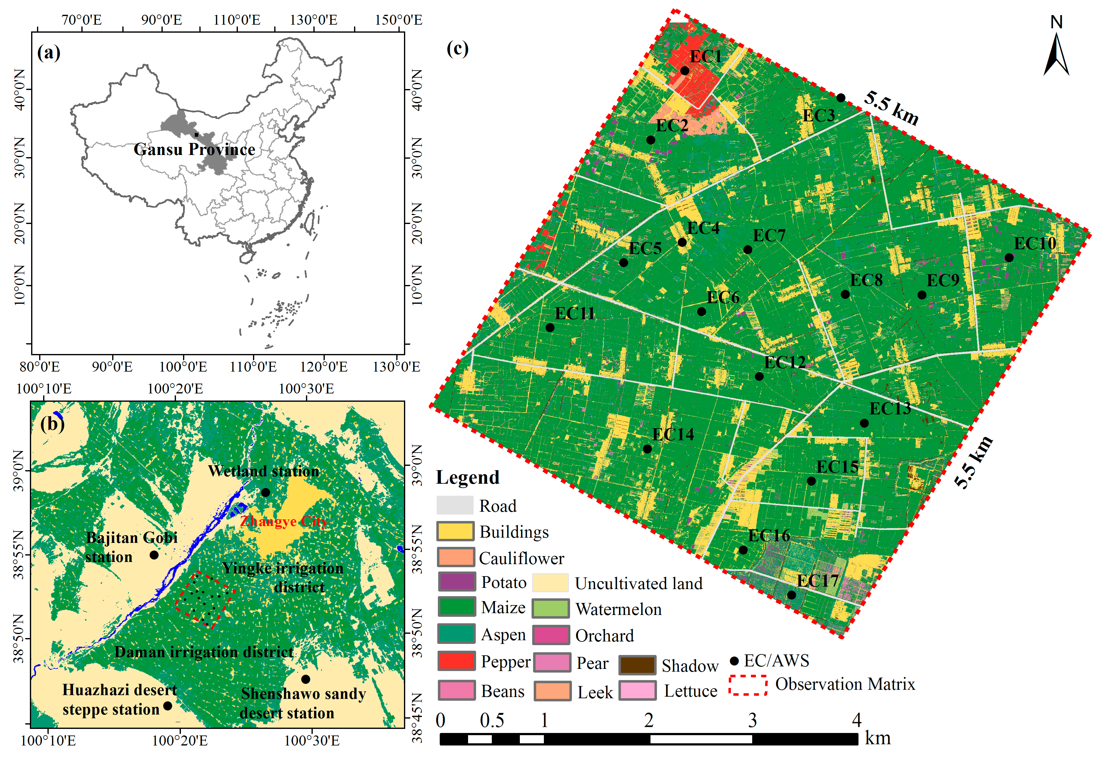
The study area (Figure 1b), which includes the Yingke and Daman irrigation districts in the Zhangye oasis and adjacent Gobi Desert, is located at 100.10°E–100.66°E, 38.68°N–39.15°N in the central reaches of the Heihe River Basin (HRB) and near the city of Zhangye in the arid region of Gansu Province in northwestern China (Figure 1a). The climate is cold and arid, with a mean annual precipitation, temperature, and potential evapotranspiration of 100–250 mm, approximately 7 °C, and 1200–1800 mm, respectively. Its terrain is flat, and its elevation is approximately 1480 m. The two irrigation districts are key experimental areas of the HiWATER project (see Li et al. [38] and Liu et al. [39] for details). One major objective of the HiWATER project, namely, the Multi-Scale Observation Experiment on Evapotranspiration (HiWATER-MUSOEXE), is to capture the strong land surface heterogeneities and associated uncertainties within a watershed [3,38,39]. The core experimental area is heterogeneous and dominated by maize, spring wheat, vegetables, orchards, and residential areas (Figure 1c).
2.2. Datasets
2.2.1. Ground Observation Data
Several ground observation datasets from HiWATER were employed in this study. HiWATER was designed as a comprehensive ecohydrological experiment to address problems that include heterogeneity, uncertainty, scaling, and closing the water cycle at the watershed scale implemented in the HRB, an inland river watershed [2]. MUSOEXE, a component of HiWATER, was implemented to reveal the spatial heterogeneities of heat and water fluxes by constructing a flux matrix (Figure 1c) from May to September 2012. The matrix includes 17 eddy covariance (EC) systems together with automatic weather stations (AWSs) that were installed in the 5.5 × 5.5 km2 kernel experimental area (Figure 1c) according to the distribution of crops, shelterbelts, roads, residential areas and canals, as well as according to soil moisture and irrigation status [39]. Among the 17 EC systems, 14 were installed in maize fields, and the other three were located in a residential area (EC4 in Figure 1c), a vegetable field (EC1 in Figure 1c) and an orchard (EC17 in Figure 1c). The EC station mainly provides flux data (including carbon dioxide flux, sensible heat flux and latent heat flux), friction wind speed, etc. Meteorological data, including air temperature and humidity, wind speed and direction, solar radiation and net radiation, layers of soil temperature and humidity, etc., were recorded at the AWSs.
The consistency of all of the EC systems and the quality of the data were ensured using the following steps. First, the consistency of the EC instruments was tested during an inter-comparison campaign in the flat, open Gobi Desert, over a surface covered by coarse grain sand and small pebbles with withered sparse scrub vegetation. This campaign was completed before HiWATER-MUSOEXE was conducted [40]. Second, all of the raw data were acquired at 10 HZ and processed using the Edire software package developed by the University of Edinburgh (Edinburgh, UK). The processing steps included spike removal, lag time correction, coordinate rotation (2D rotation), frequency response correction, corrections for density fluctuations (WPL-correction), and averaging to half-hourly fluxes [39,41]. Third, a four-step procedure was performed to control the quality of the EC data; for more details, see [1,2]. Because night turbulence is weak and considerable data are either missing or of poor quality, this study used data from 10:00 to 18:00 Beijing time to ensure the quality of turbulent flux observation data. The crop growth season is from June to September, and good quality data for 5 days were selected for each month, including 25, 26, 28–30 June; 23, 26, 27, 30 and 31 July; 4, 5, 8, 22 and 25 August; and 2, 6, 8, 12 and 14 September, for a total of 20 days.
2.2.2. Airborne Data
The remote sensing data used in this study included multiangular and multispectral images that were collected by an airborne wide-angle infrared dual-model line/area array scanner (WiDAS) and high-resolution land cover maps derived from an airborne compact airborne spectrographic imager (CASI). Land cover maps with 1-m resolution were produced by an object-oriented workflow using CASI images [42]. The landscape was classified into fourteen detailed land cover types (Figure 1c), and the results were validated using ground survey points. The overall accuracy was 88.48%, and the Kappa coefficient was 0.87 [42]. WiDAS is one of the major instruments used in the HiWATER-MUSOEXE airborne missions to acquire multiangular observation data. It acquires images using four CCD cameras in the visible near-infrared (VNIR) bands and two thermal cameras in the mid-infrared (MIR) and thermal infrared (TIR) bands. The specification payloads of WiDAS can be seen in Liu et al. [43]. For the flight data collected on 3 August 2012, 15 tracks are included in total. After calibration, lens distortion correction, geometric correction, viewing angle retrieval, and atmospheric correction, the resolutions of the visible infrared band and thermal infrared band are 0.5 m and 5 m, respectively. To ensure that each track has 750 rows × 250 columns (3750 × 1250 m2) as a prerequisite, six tracks were selected from 15 tracks. Each track is divided into three regions, each with a size of 1250 × 1250 m2 as the test area. We used pre-processed WiDAS data to calculate the LAI [1] and LST [43], and resampled the surface variable data to 5 m.
3. Methodology
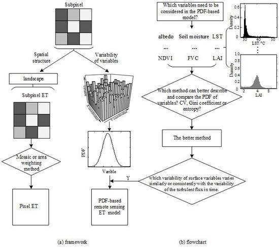
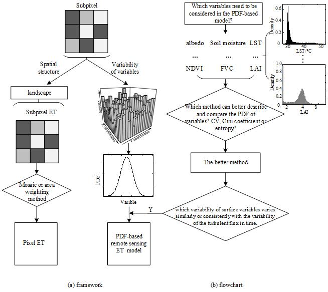
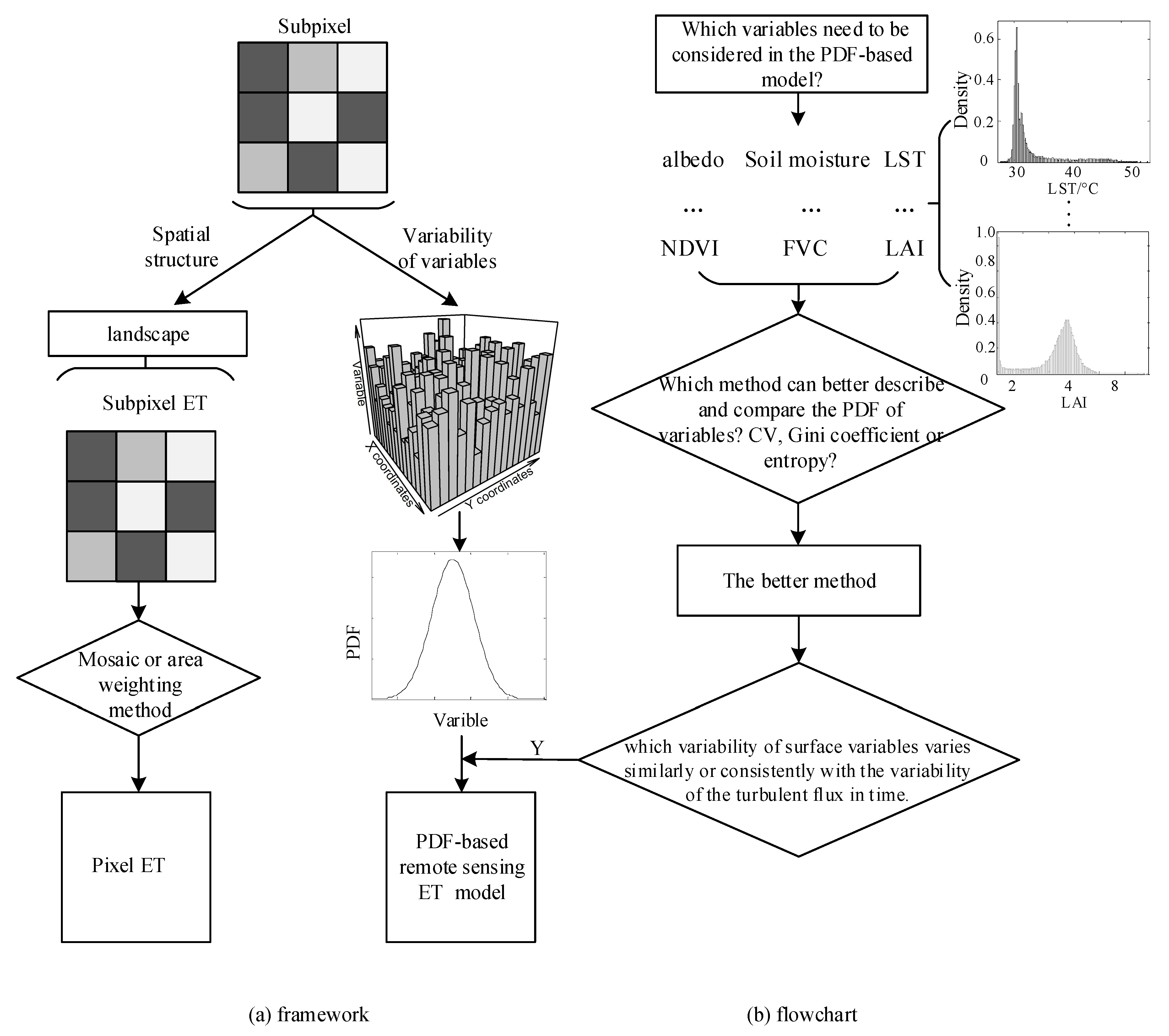
The remote sensor above the land surface receives not only the signal of the mean and variance but also the signal of all values present on the surface. Thus, modelers are especially interested in the PDF of the surface variable [14,34], which tells how frequent a certain parameter value occurs. For the same variable, if the PDF is narrow, then the surface is more homogeneous, and if the PDF is broad, the surface is more heterogeneous [34]. PDF can describe heterogeneity in a qualitative manner, however, it is unable to quantify the information content and cannot be used to compare the variability of different variables over the same observed scene [34]. As we mentioned in the introduction, the commonly used methods that express the spatial variability of surface variables include the quantile, range, deviation, variance/standard deviation, moment, CV, Gini coefficient and entropy. Because the magnitude and dimension of each surface variable vary, a dimensionless or dimensional consistent indicator is required to compare the variability between variables directly. After comparing the aforementioned methods, the indicators that can satisfy the above demand and better represent the variability are the CV, Gini coefficient and entropy. The first two are dimensionless. For a fixed scale, the amount of information can be quantified via the entropy and its dimension is consistent; the unit in this paper is nats. We illustrate the characteristics of the three methods in expressing spatial variability from both aspects of simulated data and experimental data. The framework and flowchart of this paper is shown in Figure 2. PDF is the starting point for our research of surface spatial variability. The framework in Figure 2 is as we reviewed in the introduction, and for the flowchart (i.e., the main purpose of this paper), it is the first step to answer the basic question, and also the first step to build a more efficient PDF-based ET or LE estimation model. The details of the three methods are described in the following paragraphs.
CV is dimensionless and often used for auxiliary modeling, such as the use of CV to characterize surface variability when establishing a temperature-sharpening method, and lower CV values correspond to more homogeneous land surface values [1,3,36]. CV can evaluate the variability of a sample in a population as follows [25]:
where std(x) and u(x) are the standard deviation and the average value of the sampling point, respectively. u(x) can be negative, then the above equation is also negative. However, if CV is negative, its absolute value should be used to measure the degree of variability (i.e., the greater the absolute value, the stronger the degree of variability, and vice versa). Generally, a value of CV < 0.15 indicates a variable with low variability; 0.15 ≤ CV ≤ 1 indicates a variable with moderate variability; and CV > 1 indicates a variable with a high degree of variability [1,36].
Compared to CV, the Gini coefficient is also dimensionless and is more likely to represent the ratio of deviations between data [44]. The Gini coefficient is an index of the fairness of the income distribution in the field of economics, and it is in the range of [0, 1]. For n values of the variable x, a number of methods are available to calculate the Gini coefficient. The calculation method used in this study is as follows [44]:
Information entropy is a state variable in thermodynamics that indicates the degree of chaos, and it was introduced into information theory by Shannon (sometimes called Shannon entropy) and now represents a measure of the uncertainty of a random variable. The random variable is divided into several intervals, each of which represents a state of the variable, and entropy is the average uncertainty of all possible states of the variable. It is also a common tool to quantify the information included in the PDF [34,45]. For discrete data, the formula is as follows [46]:
where pi is the probabilistic mass function (PMS) of the variable that falls within the ith interval after dividing the set of points into n intervals, and it satisfies the normalization condition . The calculation of entropy is related to the size and the start of the probability density interval segmentation, and Brunsell, Ham and Owensby [35] suggested using the kernel density estimation method to determine the interval size and the starting value. In this paper, we used the Gaussian kernel density estimation method to divide the interval into 512 aliquots and calculate the probability [47]. When the variable has only one state or a single value distribution, the entropy value is 0; and when the variable is evenly distributed, the entropy value of the variable is the largest, which is ln n.
Because the number of observations involved in the calculation of each variable varies, in order to make the variability of each variable comparable, the entropy of all variables must be normalized, and the formula is as follows:
where m is the number of observations.
The above three methods are often used in remote sensing-assisted modeling [1,3,34,44]. Therefore, compared with other methods (i.e., quantile, range, deviation, variance/standard deviation and moment) the three methods are not only dimensionless or dimensional consistent, but also have representativeness. In this paper, we analyze the three methods from different type of data (e.g., remote sensing airborne data) to express variability.
4. Results and Analysis
4.1. Analysis Based on Simulation Data
As we mentioned before, PDF is the starting point for our research of surface spatial variability. Therefore, the variability of the value of remote sensing variables is the object of this paper. The variability of different surface variables (such as LST, soil moisture, and stomatal conductance) is commonly studied using the following distribution models: normal distribution, beta distribution, gamma distribution, Weibull distribution, and exponential distribution [12,14]. To better compare the ability of the Gini coefficient, CV and entropy to express variability, we have designed three schemes from the perspective of simulation data. In Scheme 1 (see Figure 3 for details), we simulated 18 groups of random numbers with six types of distribution, all of which passed the Kolmogorov-Smirnov test at p > 0.05. The design of Scheme 1 is mainly used for the comparison of the methods within the distribution, and each group yields 10,000 random numbers to calculate the aforementioned methods. The Schemes 2 and 3 are designed to compare the three methods in describing the variability between the different distributions. However, even for the same remote sensing variable that satisfies the same distribution, the range of its value may also be different for various reasons (e.g., different acquisition times). Scheme 3 is designed to reflect this difference and is therefore more specific. The calculation results of the three methods for the simulated data in Scheme 1 are shown in Table 1.
Table 1 shows that there are some differences between the three methods (i.e., entropy, CV and Gini coefficient) in expressing spatial variability, and the trends of CV and Gini coefficient are basically the same. Through the analysis, we can find that the difference between the three methods basically occurs in the range of data values that vary greatly or with extreme data value distribution. For example, the data range of the N(3) group is larger than the other two groups in the normal distribution or three group data in the beta distribution. However, the N(3) group of PDF is broader than the other two groups, so it should be more heterogeneous, while the CV and Gini coefficient are not very stable. In addition, from the exponential distribution, the CV of the E(2) group is larger than the CV of the E(3) group, whereas the Gini coefficient is the opposite. Combined with Figure 3, it can be found that the PDF distribution of E(3) group is more concentrated, which indicates that it is more homogeneous. Gini coefficient is more likely to represent the ratio of deviations between data [44], so it is worse than the CV when expressing the variability.
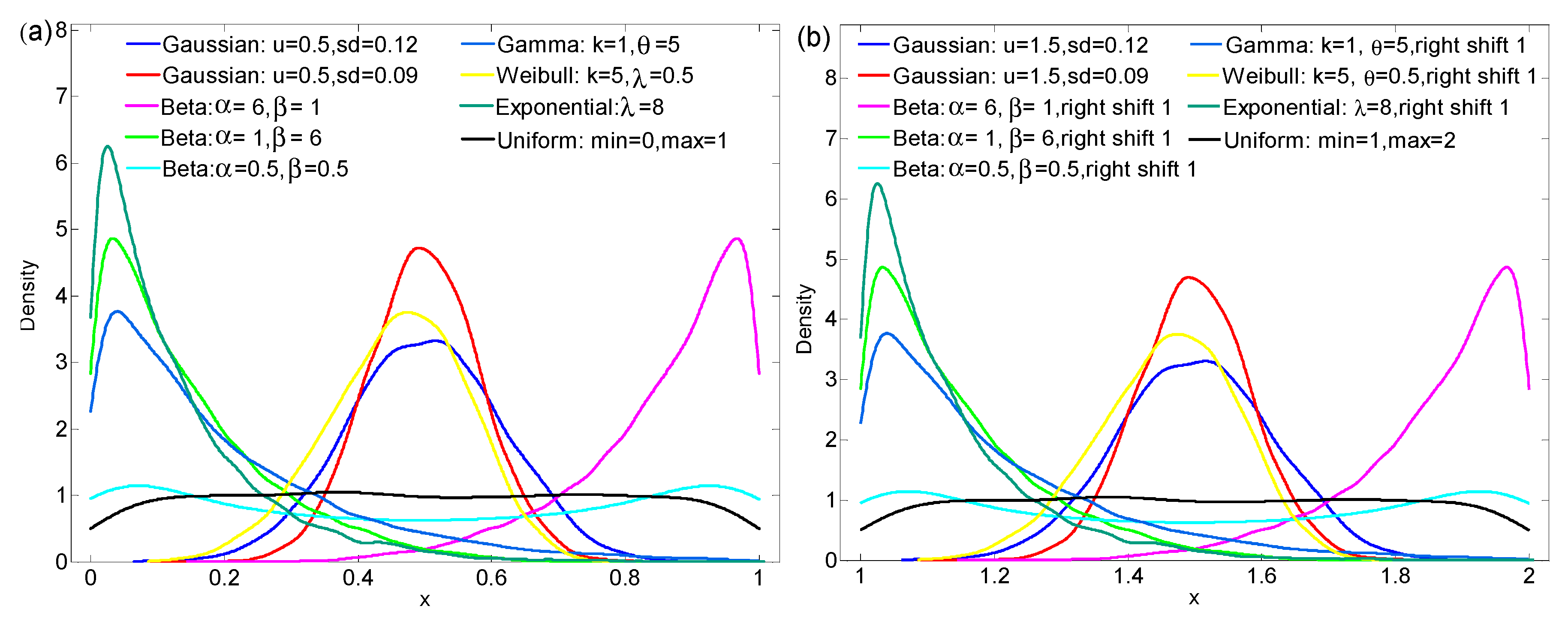
To compare the three methods in describing the variability between the different distributions, we designed Scheme 2. The data of Scheme 2 are the nine groups of data that are in the same interval (i.e., [0, 1]) selected in Scheme 1. These nine sets of data also cover six distributions, and their PDF distributions are shown in Figure 4. The nine groups of data in Scheme 2 represent the different variability distributions: the variability represented by (a) is stronger than that represented by (b); (c) and (d) represent a large number of uniform data mixed with a small amount of non-uniform data, but their spatial variability is basically the same; (e) represents a bimodal distribution; (f) and (h) are similar to (d), and (g) is similar to (a); (i) is an extreme case with a maximum variability, where the uniform distribution of (i) refers to the probability that the spatial distribution of the data is uniform, which is completely opposite to the uniform distribution of surface variables in the study of remote sensing (the uniform distribution in remote sensing usually refers to a single value distribution, that is, the entire study area has only one value). Combined with Figure 4a, the variability of these data is roughly sorted as follows: (i) > (e) > (f) > (c) ≈ (d) > (h); (a) > (g) > (b). The entropy is calculated in the same way as the interval division of the data in group (i), and the calculation results of the three methods are shown in Table 2. We can find that the results of the entropy can better reflect the variability of the data in Scheme 2, while the results of CV and Gini coefficient are not very stable. For example, the variability of (c) and (d) is basically the same, whereas the results of the CV and the Gini coefficient vary considerably. The reason is that CV and Gini coefficient are affected by the values of the variable. To confirm this, we designed Scheme 3.
In Scheme 3, we add 1 to the original random number generated in Scheme 2 so that the interval range becomes [1, 2], as shown in Figure 4b. The variability of each simulated data in Scheme 3 is also calculated using three methods, and the results are shown in Table 3. The data in Scheme 3 have the same variability as in Scheme 2, and the standard deviation is also the same. However, from the calculation results, only the value of entropy is unchanged, and the CV and Gini coefficient results undergo great changes. Thus, the CV and Gini coefficient are influenced by the variable values, specifically the mean of the variables, which can be seen via the calculation equations of the two [25,44].
From a comprehensive comparison of Table 1, Table 2 and Table 3, we can find that: (1) the variation range of entropy is larger than that of the CV and Gini coefficient, although the magnitude fluctuation of entropy is smaller than that of the other two; (2) the variation trend of the CV is consistent with that of the Gini coefficient; (3) for non-extreme cases, the entropy, CV and the Gini coefficient can be a good measure of the degree of discretization, such as (a) and (b) in Schemes 2 and 3; (4) however, for extreme cases, the CV and the Gini coefficient are less effective than the entropy value for measuring spatial fluctuations, for example, the fluctuation degree of (i) is the largest but the CV and Gini coefficient values are smaller than (d) and (e) in Scheme 2; moreover, the variability of (c) and (d) is basically the same, whereas the results of the CV and Gini coefficient vary considerably in both Schemes 2 and 3; and (5) the entropy values are relatively stable and do not change with the value of the variable given for the same distribution, whereas the CV and Gini coefficient values are easily affected by the variable mean value. Specifically, when the range of variable values in Scheme 3 changes, the entropy values remain unchanged, while the CV and the Gini coefficient change greatly. From the analysis of the simulated data, we can draw the preliminary conclusion that entropy can better describe the spatial fluctuation than the other two methods, and it is more suitable for the comparison of variability among different variables.
4.2. Analysis Based on Field Experimental Data
4.2.1. Analysis Based on Airborne Data
As mentioned in Section 2.2.2, we divided the selected tracks into three equal areas, with each containing 250 × 250 pixels. The LAI and LST of each track are retrieved respectively. The CV, Gini coefficient and entropy of each variable in each region were calculated, and the calculation results are shown in Table 4. In addition, the corresponding land cover maps for each region is obtained.
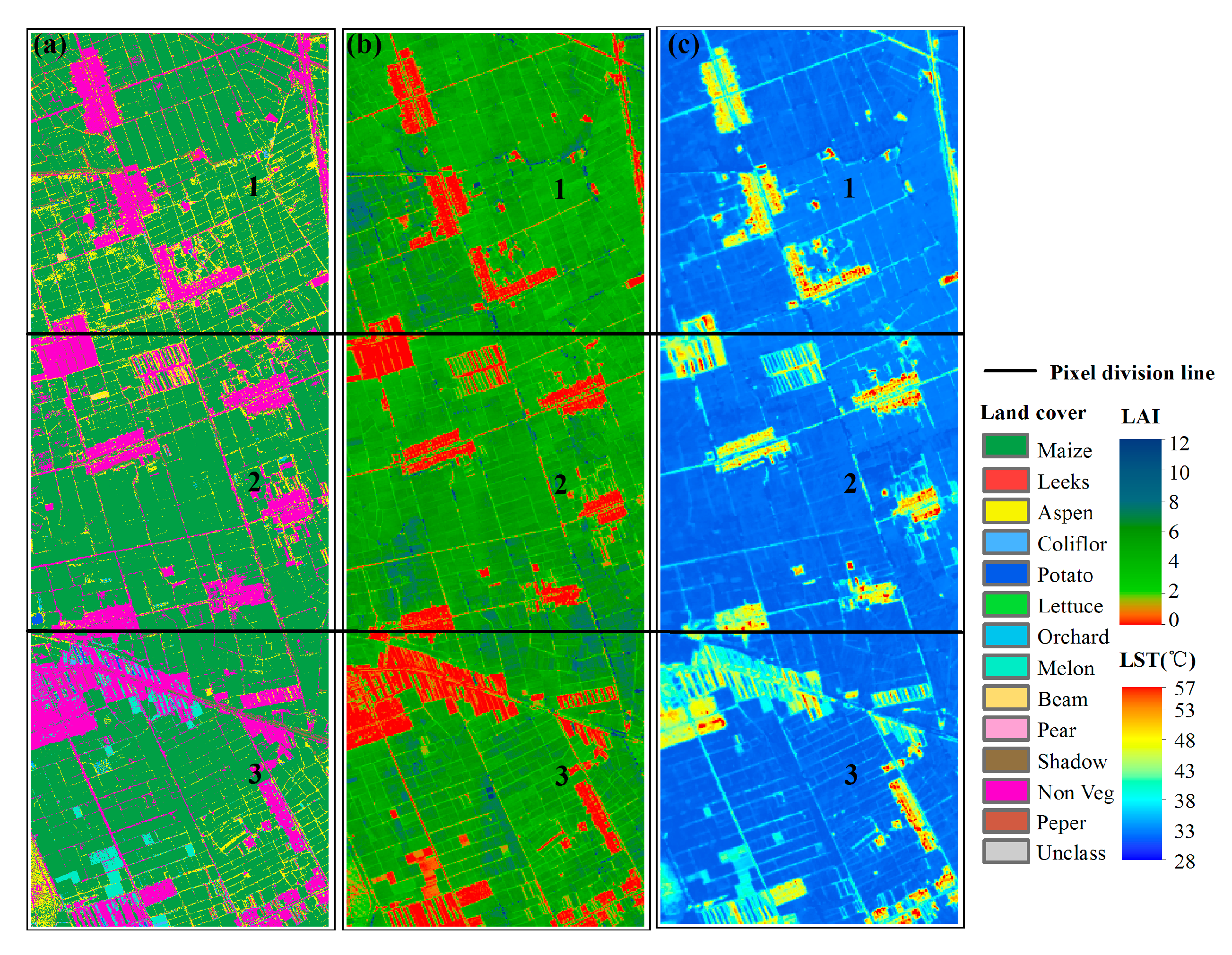
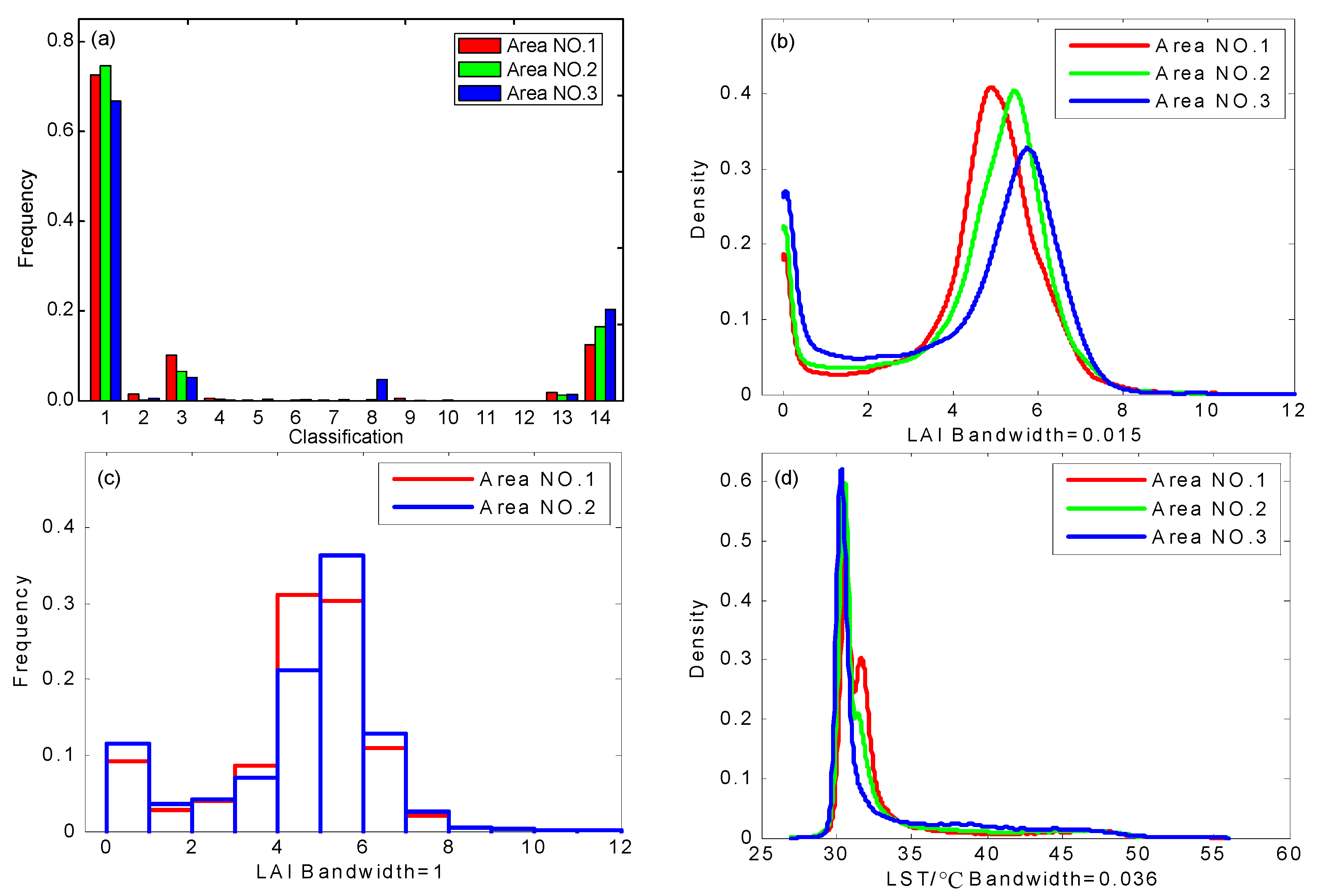
Taking track 5-1 as an example, the experimental area corresponds to Area NO. 1–Area NO. 3. The spatial distribution of the variables and the surface types of the three study areas are shown in Figure 5. The area (pixel number) proportion of vegetated, shadow and non-vegetated areas were 0.858:0.016:0.126 (53,634:1018:7848); 0.825:0.01:0.165 (51,554:633:10,313) and 0.784:0.01:0.206 (49,001:559:12,900), respectively, which resulted in a larger variation of the variable range. Figure 6 is the probability density distribution of the surface variables (i.e., LAI and LST) and the surface types. The proportion of vegetated area (especially corn area) is large; therefore, the distribution of variables is concentrated. Combined with Table 4, the following conclusions can be drawn.
- (1)
- Figure 6b shows that the LAI values of the three study areas are mainly distributed near 0 and high value (between 4.0 and 7.0), thus showing a bimodal distribution. For the LAI, the CV and Gini coefficient calculation results show that Area NO. 2 has more variation than Area NO. 1, although the entropy results show that Area NO. 1 is more variable. A comparison of the frequency distribution histograms (bandwidth = 1) of LAI in the two study areas (Figure 6c) shows that the LAI peak width of Area NO. 2 is narrower, meaning that the probability distribution of LAI in Area NO. 2 is more concentrated; therefore, the entropy of Area NO. 2 is smaller than that of Area NO. 1. Moreover, the proportion of non-vegetated area (LAI = 0) in Area NO. 2 is larger, which results in a widened standard deviation and a lower mean. Therefore, the calculated CV and Gini coefficient results are relatively large. However, the spatial variability of LAI in Area NO. 1 is greater overall than that in Area NO. 2.
- (2)
- The LST range of Area NO. 1~Area NO. 3 is nearly 30 °C, and the distribution of the values is mainly between 30~35 °C (Figure 6d). For the LST, the entropy, CV and Gini coefficient calculation results are consistent and all are incremental; thus, the LST variability of the three study areas is as follows: Area NO. 3 > Area NO. 2 > Area NO. 1.
- (3)
- For the variability of variables, LAI > LST. Although the value range of LST is larger than that of LAI, the variability of LAI is larger than that of LST, which can be directly obtained via calculations using the three methods.
- (4)
- The variability of LST seems to have a certain relationship with the variability of LAI, in this paper, the LST-LAI variability is negative. Because of the complex relationship between vegetation information and LST (e.g., NDVI-LST) [48], the correlation between the two variabilities needs to be further studied.
Figure 7 shows the variation of the three methods as the range of the LST increases (i.e., the number of pixels increases gradually). The trend of the three methods is similar. In the range of 5–300 m, the curve changes steeply, and the slope is large, which is due to additional points caused by the new mixed other types of land or the growth of large differences in vegetation, so the variability in the study area increases rapidly. In the range of 300–800 m, the variability of the variable tends to be stable, which may be related to the optimal scale [19]. From the perspective of probability density distribution, the scale range increases, which leads to more occurrences of the variable in a certain range (state), that is, the probability is greater, indicating that the value of the variable is more concentrated and more dominant than other states, so its spatial variability remains stable or even reduces.
For the LAI in our study area, as the scale range increases, the following occurs: (1) when the dominant land cover of the pixel is covered by buildings or bare soil and only a very small number of pixels or individual pixels are vegetation cover, the value of LAI is largely zero and only a small number of non-zero values are observed; or (2) only a small amount of the pixel is covered with buildings or bare soil and these land types are mixed with a large number of vegetation area; thus, the value of LAI is largely non-zero. These two cases often occur with mixed pixels, such as at the junction of farms and villages. In such situations, the pixels are obviously relatively pure, the spatial variability is relatively weak, but the CV values in case (1) are much larger than those in case (2) and the Gini coefficient values are close to 1 and 0 in both cases. However, the entropy values are consistent in both cases, which is similar to cases (c) and (d) in Schemes 2 and 3 of the simulated data described in Section 4.1. These findings show that the CV and the Gini coefficient are insufficient for measuring spatial variability. Because the Gini coefficient is not ideal, the calculation is large and the trend is similar to that of the CV; thus, the following analyses will no longer consider the Gini coefficient.
4.2.2. Analysis Based on Ground Observation Data
The variables that can be analyzed using airborne data are limited, and ground observation data (i.e., AWSs and ECs) can provide multivariate continuous observation data, which are beneficial for analyzing the overall variability of each variable and its temporal variation. Nine surface variables are analyzed in this section, and the number of observations for each variable is shown in Table 5.
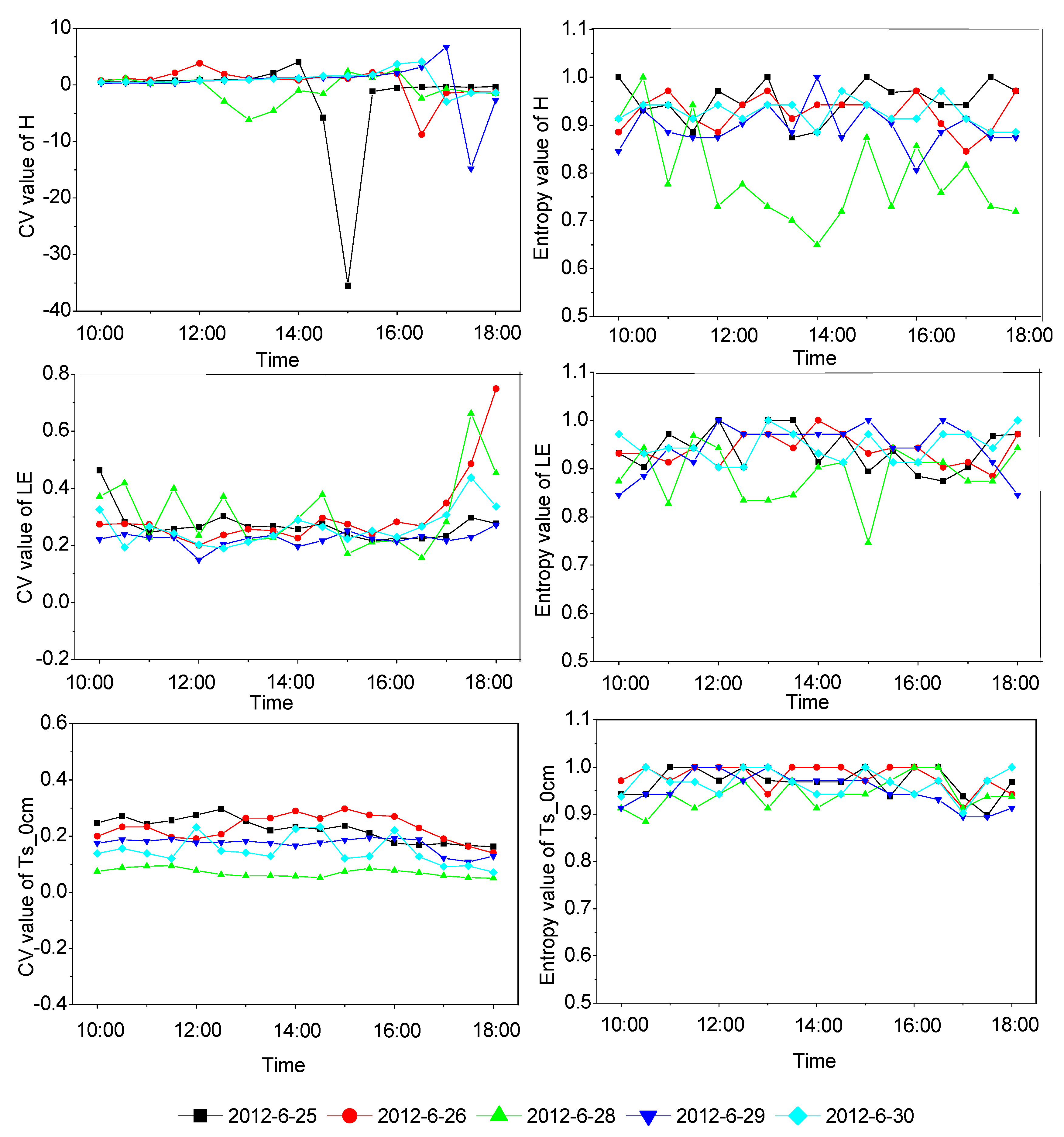
Among them, H, LE, and Ustar were observed by the EC systems and RH_5m, Ta_5m, Ms_2cm, Rn and Ts_0cm were observed by the AWS stations. Because one of the stations (i.e., EC16) lacked radiation observation data, the albedo and Rn have only 16 observation data. To make the variability of each variable comparable, the entropy of each variable needs to be normalized according to Equation (4). The normalized entropy and CV are calculated from the half-hourly of ground observation data processed in Section 2.2.1. Taking the surface variables (i.e., H, LE and Ts_0cm) from June 2012 as an example, the variation in entropy and CV with time is shown in Figure 8. The evaporation from crops is greater during the growing season, and the value of the sensible heat flux (H) is much smaller than that of the latent heat flux (LE). Studies have shown that at an oasis in the summer, a temperature inversion occurs [1,2,3], and H is sometimes less than 0 and its mean is close to 0 or even negative. In addition, the CV values are large and the variation is intense; therefore, the CV values of H are unstable. This situation is similar to that described in Section 4.1, meaning that a large number of zero values are mixed with non-zero values. In contrast, entropy values do not change dramatically because entropy does not consider the specific size of the variable value and is only related to the frequency of the variable value within a certain interval. In addition, the CV values of H show that the turbulence flux spatial fluctuation is relatively small at approximately 11:00 a.m. because with solar radiation enhancement, the surface begins to heat up, evapotranspiration increases, and the H spatial variation changes are stable. However, in the afternoon, the oasis effect appears, and H is negative for the observation site and gradually increases, resulting in CV values that begin to fluctuate violently. Figure 8 shows that the CV values and entropy values of the LE variations are also more intense. Furthermore, the trend of H and LE seems to show a certain diurnal variation and this requires further detailed study.
Table 6 shows the statistics of entropy calculated for the nine variables over 20 days. It can be seen that the entropy of Ms_2cm is the largest. The reason may be due to that the LE has a strong variability and is relatively discrete (STD = 0.048), coupled with other factors such as wind speed, resulting in significant differences in evapotranspiration [2]. Thus, the distribution of surface soil moisture is quite different. Followed by Ustar and Ts_0cm, they also have strong variability. The reason for the entropy of Ustar being higher may be related to the influence of surface geometry and atmospheric conditions on wind speed; the HiWATER-MUSOEXE test area is surrounded by HRB and the Gobi Desert (Figure 1b), so the spatial variation of the wind speed is large. For the soil temperature at 0 cm (Ts_0cm), there is a high degree of spatial variability because of the influence of surface humidity and the shadow of each observation site. In general, the evaluation of entropy as a representation of variability is more credible than that of the CV.
5. Discussion
The entropy describes the spatial variability much better than CV and Gini coefficient. Generally, the CV and Gini coefficient have similar characteristics when expressing spatial variability, but the Gini coefficient is more focused on the deviation ratio between data. Therefore, in some cases, the Gini coefficient is worse than the CV in expressing spatial variability, and the Gini coefficient has a large computational effort. In summary, the advantages of entropy are described as follows:
- Entropy is more consistent with PDF when describing spatial variability, and in some extreme distributions, entropy can express spatial variability more accurately, while CV and Gini coefficients cannot.
- In this paper, the unit of entropy is nats, which can be used directly to compare the spatial variability of variables. While the CV and Gini coefficients cannot, they are affected by the specific value (i.e., the average) of the variable.
Nevertheless, it is worth mentioning that PDF is the starting point for our research of surface spatial variability. If we do not use this as a prerequisite to analyze the heterogeneity of surface variables separately, the spatial patterns (also known as spatial structure) or spatial autocorrelation of the surface must be considered [26,34]. Entropy calculates the variability of variables in their own range. In Table 1, if we compare the three methods in describing the variability between the different distributions, the result is still reliable. However, we must consider the actual range of variables. For example, if variable A satisfies a uniform distribution, its value can range from 0 to 10, and in some cases (e.g., an observation scene of a remote sensing image or the target area that we are interested in) its value falls in the range of 0–1. If there is no value in the 1–10 range, similar to U (1) in Table 1, then its variability is not necessarily stronger than variable B which belongs to other distributions (e.g., the beta distribution in Table 1) in the actual sense. In this article, the design and arrangement of the scheme is to gradually illustrate the characteristics of the three methods in expressing spatial variability. In addition, entropy takes into account the distribution of variable values, and its calculation has a certain dependence on the number of samples. Considering the high cost of the experiments, the datasets of the seventeen EC systems and AWS stations in the 5.5 × 5.5 km2 kernel experimental area are very valuable [39]. Moreover, the conclusions drawn from the analysis based on the spatial data may be quite preliminary but are important and valuable for future exploration in this area. More data from wireless sensor network [49] will be added and used for more sophisticated analysis. More reliable and interesting findings will be discovered with increased number of sites and observations. Detailed information on the spatial variability of variables derived from the ground observation network and the time variation of the variability of surface variables will be introduced in another paper.
6. Conclusions
The estimation of ET or LE using remote sensing data does not usually consider the influence of advection or interaction between subpixels; hence, the distribution of surface variable values (i.e., spatial variability) is usually the focus for building a model that considers the heterogeneity produced by surface variables for a target area or landscape. PDF is the most promising way to describe subpixel variability for given data. In attempting to produce efficient PDF-based parameterization of remotely sensed ET or LE, it is important to determine which variables are similar or consistent with the variability of turbulent flux in time. However, the use of PDF alone does not facilitate direct comparisons of the spatial variability of surface variables. To address this, we chose three dimensionless or dimensional consistent indicators, i.e., CV, Gini coefficient and entropy values, to express the variability in surface variables. Based on the analysis of simulated data and the field experiment data, we found the following: (1) Entropy has a high consistency with the PDF of surface variables, which is more stable and efficient in expressing the variability of surface variables. The entropy of the airborne data shows that the variability of LAI is greater than that of LST; (2) Regardless of whether it is from the analysis of simulated data or field experimental data, the CV and the Gini coefficient are insufficient for measuring spatial variability. They are susceptible to the mixing of special values, such as the inversion of temperature at the oasis in the summer; (3) The results of normalized entropy of different variables observed by EC systems and AWS stations show that the variability of soil moisture at depth of 2 cm (MS_2cm) is the strongest, and the variability of friction wind speed (Ustar) is relatively strong, which is related to the special geographical environment of the study area. Furthermore, the trend of sensible heat flux (H) and latent heat flux (LE) seems to show a certain diurnal variation.
The findings of this study provide a reference for expressing the spatial variability of surface variables and illustrate a suitable method for comparing the variability of different variables. How to combine it with the analysis in which surface variables vary similarly or consistently with the variability of the turbulent flux in time and to establish a more efficient PDF-based remote sensing ET or LE model will be the next research goal.
Acknowledgments
This study was jointly supported by the Chinese Natural Science Foundation Project (grant No. 41371360) and the Special Fund of the Chinese Academy of Sciences (grant No. KZZD-EW-TZ-18). We are grateful to Prof. Qing Xiao of Institute of Remote Sensing and Digital Earth Chinese Academy of Sciences, Beijing, China for providing the WiDAS data. In addition, we thank all of the scientists and engineers who took part in the HiWATER experiment. We also thank the reviewers and editors for their insightful and constructive comments.
Author Contributions
Xiaozhou Xin provided the ideas for this work; Xiaozhou Xin, Xiaojun Li and Zhiqing Peng prepared the manuscript and designed the experiments; Xiaojun Li and Hailong Zhang performed the experiments; Chuanxiang Yi, and Bin Li collected and processed the data. Xiaozhou Xin participated in discussions and revising the manuscript; Xiaojun Li wrote the paper. These authors contributed equally.
Conflicts of Interest
The authors declare no conflict of interest.
References
- Peng, Z.Q.; Xin, X.Z.; Jiao, J.J.; Zhou, T.; Liu, Q.H. Remote sensing algorithm for surface evapotranspiration considering landscape and statistical effects on mixed pixels. Hydrol. Earth Syst. Sci. 2016, 20, 4409–4438. [Google Scholar] [CrossRef]
- Wang, Y.Q.; Xiong, Y.J.; Qiu, G.Y.; Zhang, Q.T. Is scale really a challenge in evapotranspiration estimation? A multi-scale study in the Heihe oasis using thermal remote sensing and the three-temperature model. Agric. For. Meteorol. 2016, 230–231, 128–141. [Google Scholar] [CrossRef]
- Li, X.J.; Xin, X.Z.; Jiao, J.J.; Peng, Z.Q.; Zhang, H.L.; Shao, S.S.; Liu, Q.H. Estimating subpixel surface heat fluxes through applying temperature-sharpening methods to MODIS data. Remote Sens. 2017, 9, 836. [Google Scholar] [CrossRef]
- Jacob, F.; Weiss, M. Mapping biophysical variables from solar and thermal infrared remote sensing: Focus on agricultural landscapes with spatial heterogeneity. IEEE Geosci. Remote Sens. Lett. 2016, 11, 1844–1848. [Google Scholar] [CrossRef]
- Kustas, W.; Li, F.; Jackson, T.; Prueger, J.; MacPherson, J.; Wolde, M. Effects of remote sensing pixel resolution on modeled energy flux variability of croplands in Iowa. Remote Sens. Environ. 2004, 92, 535–547. [Google Scholar] [CrossRef]
- Kustas, W.P.; Norman, J.M. Evaluating the effects of subpixel heterogeneity on pixel average fluxes. Remote Sens. Environ. 2000, 74, 327–342. [Google Scholar] [CrossRef]
- Arain, A.M.; Michaud, J.; Shuttleworth, W.J.; Dolman, A.J. Testing of vegetation parameter aggregation rules applicable to the Biosphere Atmosphere Transfer Scheme (BATS) and the FIFE site. J. Hydrol. 1996, 177, 1–22. [Google Scholar] [CrossRef]
- Chehbouni, A.; Njoku, E.; Lhomme, J.; Kerr, Y. Approach for averaging surface parameters and fluxes over heterogeneous terrain. J. Clim. 1995, 8, 1386–1393. [Google Scholar] [CrossRef]
- Koster, R.D.; Suarez, M.J. A comparative analysis of two land surface heterogeneity representations. J. Clim. 1992, 5, 1379–1390. [Google Scholar] [CrossRef]
- Li, B.; Avissar, R. The impact of spatial variability of land-surface characteristics on land-surface heat fluxes. J. Clim. 1994, 7, 527–537. [Google Scholar] [CrossRef]
- Blyth, E.M.; Harding, R.J. Application of aggregation models to surface heat flux from the Sahelian tiger bush. Agric. For. Meteorol. 1995, 72, 213–235. [Google Scholar] [CrossRef]
- Avissar, R. Conceptual aspects of a statistical-dynamical approach to represent landscape subgrid-scale heterogeneities in atmospheric models. J. Geophys. Res. Atmos. 1992, 97, 2729–2742. [Google Scholar] [CrossRef]
- Maayar, M.E.; Chen, J.M. Spatial scaling of evapotranspiration as affected by heterogeneities in vegetation, topography, and soil texture. Remote Sens. Environ. 2006, 102, 33–51. [Google Scholar] [CrossRef]
- Tittebrand, A.; Berger, F. Spatial heterogeneity of satellite derived land surface parameters and energy flux densities for LITFASS-area. Atmos. Chem. Phys. 2009, 9, 16219–16254. [Google Scholar] [CrossRef]
- Mölders, N.; Raabe, A. Numerical investigations on the influence of subgrid-scale surface heterogeneity on evapotranspiration and cloud processes. J. Appl. Meteorol. 1996, 35, 782–795. [Google Scholar] [CrossRef]
- Norman, J.M.; Anderson, M.C.; Kustas, W.P.; French, A.N.; Mecikalski, J.; Torn, R.; Diak, G.R.; Schmugge, T.J.; Tanner, B.C.W. Remote sensing of surface energy fluxes at 101-m pixel resolutions. Water Resour. Res. 2003, 39. [Google Scholar] [CrossRef]
- Bayala, M.I.; Rivas, R.E. Enhanced sharpening procedures on edge difference and water stress index basis over heterogeneous landscape of sub-humid region. Egypt. J. Remote Sens. Space Sci. 2014, 17, 17–27. [Google Scholar] [CrossRef]
- Mukherjee, S.; Joshi, P.K.; Garg, R.D. A comparison of different regression models for downscaling Landsat and MODIS land surface temperature images over heterogeneous landscape. Adv. Space Res. 2014, 54, 655–669. [Google Scholar] [CrossRef]
- Wu, H.; Tang, B.H.; Li, Z.L. Impact of nonlinearity and discontinuity on the spatial scaling effects of the leaf area index retrieved from remotely sensed data. Int. J. Remote Sens. 2013, 34, 3503–3519. [Google Scholar] [CrossRef]
- Zeng, X.M.; Zhao, M.; Su, B.K.; Tang, J.P.; Zheng, Y.Q.; Zhang, Y.J.; Chen, J. Effects of the land-surface heterogeneities in temperature and moisture from the “combined approach” on regional climate: A sensitivity study. Glob. Planet. Chang. 2003, 37, 247–263. [Google Scholar] [CrossRef]
- Giorgi, F. An approach for the representation of surface heterogeneity in land surface models. Part II: Validation and sensitivity experiments. Mon. Weather Rev. 1997, 125, 1900–1919. [Google Scholar] [CrossRef]
- Yeh, P.J.F.; Eltahir, E.A.B. Representation of water table dynamics in a land surface scheme. Part I: Model development. J. Clim. 2005, 18, 1861–1880. [Google Scholar] [CrossRef]
- Giorgi, F. An approach for the representation of surface heterogeneity in land surface models. Part I: Theoretical framework. Mon. Weather Rev. 1997, 125, 1885–1899. [Google Scholar] [CrossRef]
- Wang, Q.; Ni, J.; Tenhunen, J. Application of a geographically-weighted regression analysis to estimate net primary production of Chinese forest ecosystems. Glob. Ecol. Biogeogr. 2010, 14, 379–393. [Google Scholar] [CrossRef]
- Odongo, V.; Hamm, N.; Milton, E. Spatio-temporal assessment of Tuz Gölü, Turkey as a potential radiometric vicarious calibration site. Remote Sens. 2014, 6, 2494–2513. [Google Scholar] [CrossRef]
- Garrigues, S.; Allard, D.; Baret, F.; Weiss, M. Quantifying spatial heterogeneity at the landscape scale using variogram models. Remote Sens. Environ. 2006, 103, 81–96. [Google Scholar] [CrossRef]
- Wang, J.F.; Zhang, T.L.; Fu, B.J. A measure of spatial stratified heterogeneity. Ecol. Indic. 2016, 67, 250–256. [Google Scholar] [CrossRef]
- Rahman, A.F.; Gamon, J.A.; Sims, D.A.; Schmidts, M. Optimum pixel size for hyperspectral studies of ecosystem function in southern California chaparral and grassland. Remote Sens. Environ. 2003, 84, 192–207. [Google Scholar] [CrossRef]
- Haralick, R.M.; Shanmugam, K.S. Combined spectral and spatial processing of ERTS imagery data. Remote Sens. Environ. 1974, 3, 3–13. [Google Scholar] [CrossRef]
- Csillag, F.; Kabos, S. Wavelets, boundaries, and the spatial analysis of landscape pattern. Écoscience 2002, 9, 177–190. [Google Scholar] [CrossRef]
- Qiu, B.W.; Zeng, C.Y.; Cheng, C.C.; Tang, Z.H.; Gao, J.Y.; Sui, Y.P. Characterizing landscape spatial heterogeneity in multisensor images with variogram models. Chin. Geogr. Sci. 2014, 24, 317–327. [Google Scholar] [CrossRef]
- Cosh, M.H.; Brutsaert, W. Microscale structural aspects of vegetation density variability. J. Hydrol. 2003, 276, 128–136. [Google Scholar] [CrossRef]
- Zhang, L.J.; Ma, Z.H.; Luo, G. An evaluation of spatial autocorrelation and heterogeneity in the residuals of six regression models. For. Sci. 2009, 55, 533–548. [Google Scholar]
- Hintz, M.; Lennartz-Sassinek, S.; Liu, S.F.; Shao, Y.P. Quantification of land-surface heterogeneity via entropy spectrum method. J. Geophys. Res. Atmos. 2014, 119, 8764–8777. [Google Scholar] [CrossRef]
- Brunsell, N.A.; Ham, J.M.; Owensby, C.E. Assessing the multi-resolution information content of remotely sensed variables and elevation for evapotranspiration in a tall-grass prairie environment. Remote Sens. Environ. 2008, 112, 2977–2987. [Google Scholar] [CrossRef]
- Kustas, W.P.; Norman, J.M.; Anderson, M.C.; French, A.N. Estimating subpixel surface temperatures and energy fluxes from the vegetation index–radiometric temperature relationship. Remote Sens. Environ. 2003, 85, 429–440. [Google Scholar] [CrossRef]
- Wang, D.; Wang, G.; Anagnostou, E.N. Use of satellite-based precipitation observation in improving the parameterization of canopy hydrological processes in land surface models. J. Hydrometeorol. 2005, 6, 745–763. [Google Scholar] [CrossRef]
- Li, X.; Cheng, G.; Liu, S.; Xiao, Q.; Ma, M.; Jin, R.; Che, T.; Liu, Q.; Wang, W.; Qi, Y. Heihe watershed allied telemetry experimental research (HiWATER): Scientific objectives and experimental design. Bull. Am. Meteorol. Soc. 2013, 94, 1145–1160. [Google Scholar] [CrossRef]
- Liu, S.M.; Xu, Z.W.; Song, L.S.; Zhao, Q.Y.; Ge, Y.; Xu, T.R.; Ma, Y.F.; Zhu, Z.L.; Jia, Z.Z.; Zhang, F. Upscaling evapotranspiration measurements from multi-site to the satellite pixel scale over heterogeneous land surfaces. Agric. For. Meteorol. 2016, 230, 97–113. [Google Scholar] [CrossRef]
- Xu, Z.W.; Liu, S.M.; Li, X.; Shi, S.J.; Wang, J.M.; Zhu, Z.L.; Xu, T.R.; Wang, W.Z.; Ma, M.G. Intercomparison of surface energy flux measurement systems used during the HiWATER-MUSOEXE. J. Geophys. Res. Atmos. 2013, 118, 13140–13157. [Google Scholar] [CrossRef]
- Ran, Y.H.; Li, X.; Sun, R.; Kljun, N.; Zhang, L.; Wang, X.F.; Zhu, G.F. Spatial representativeness and uncertainty of eddy covariance carbon flux measurements for upscaling net ecosystem productivity to the grid scale. Agric. For. Meteorol. 2016, 230–231, 114–124. [Google Scholar] [CrossRef]
- Li, W.; Niu, Z.; Huang, N.; Wang, C.; Gao, S.; Wu, C. Airborne LiDAR technique for estimating biomass components of maize: A case study in Zhangye City, Northwest China. Ecol. Indic. 2015, 57, 486–496. [Google Scholar] [CrossRef]
- Liu, Q.; Yan, C.Y.; Xiao, Q.; Yan, G.J.; Fang, L. Separating vegetation and soil temperature using airborne multiangular remote sensing image data. Int. J. Appl. Earth Obs. Geoinf. 2012, 17, 66–75. [Google Scholar] [CrossRef]
- Valbuena, R.; Maltamo, M.; Mehtätalo, L.; Packalen, P. Key structural features of boreal forests may be detected directly using L-moments from airborne lidar data. Remote Sens. Environ. 2017, 194, 437–446. [Google Scholar] [CrossRef]
- Journel, A.G.; Deutsch, C.V. Entropy and spatial disorder. Math. Geol. 1993, 25, 329–355. [Google Scholar] [CrossRef]
- Shannon, C.E. A mathematical theory of communication. Bell Syst. Tech. J. 1948, 27, 379–423. [Google Scholar] [CrossRef]
- Silverman, B.W. Density estimation in the exploration and presentation of data. In Density Estimation for Statistics and Data Analysis, 1st ed.; CRC Press: Boca Raton, FL, USA, 1986; pp. 2–4. [Google Scholar]
- Raynolds, M.K.; Comiso, J.C.; Walker, D.A.; Verbyla, D. Relationship between satellite-derived land surface temperatures, arctic vegetation types, and NDVI. Remote Sens. Environ. 2008, 112, 1884–1894. [Google Scholar] [CrossRef]
- Jin, R.; Li, X.; Yan, B.; Li, X.; Luo, W.; Ma, M.; Guo, J.; Kang, J.; Zhu, Z.; Zhao, S. A nested ecohydrological wireless sensor network for capturing the surface heterogeneity in the midstream areas of the Heihe River Basin, China. IEEE Geosci. Remote Sens. Lett. 2014, 11, 2015–2019. [Google Scholar] [CrossRef]
Figure 1.
Geographical information of the study area: (a) schematic of Zhangye city and middle Heihe River Basin; (b) locations of HiWATER-MUSOEXE observation matrix; (c) detailed locations of the 17 EC systems and AWSs inside the Zhangye oasis. EC/AWS is the abbreviation for eddy covariance/automatic weather station.

Figure 2.
Framework and flowchart of this paper.

Figure 3.
The PDF distribution of simulated data in Scheme 1. (a–f) refer to Gaussian distribution, beta distribution, gamma distribution, weibull distribution, exponential distribution and uniform distribution, respectively.
Figure 3.
The PDF distribution of simulated data in Scheme 1. (a–f) refer to Gaussian distribution, beta distribution, gamma distribution, weibull distribution, exponential distribution and uniform distribution, respectively.

Figure 4.
The PDF distribution of simulated data: (a) Scheme 2; (b) Scheme 3.

Figure 5.
Data for each region on track 5-1: (a) 1-m classification data derived from CASI and (b) LAI and (c) LST retrieved by WiDAS.
Figure 5.
Data for each region on track 5-1: (a) 1-m classification data derived from CASI and (b) LAI and (c) LST retrieved by WiDAS.

Figure 6.
Probability density distribution and histogram of the surface variables and the surface types in three study areas: (a) histogram of 1-m classification data; (b) probability density distribution of LAI; (c) frequency distribution histograms of LAI (bandwidth = 1); and (d) probability density distribution of LST. Note: in the classification histogram, the values 1–14 represent maize, leeks, aspen, cauliflower, potato, lettuce, orchard, melon, beam, pear, peper, unclass, shadow and non-veg, respectively.

Figure 7.
Variation of the three methods when the LST scale is expanded. Note: The abscissa indicates the length of the study area that gradually increases from the upper left corner of Figure 5c with a gradient of pixels 5i × 5i (i = 0, 1, 2 … 50).
Figure 7.
Variation of the three methods when the LST scale is expanded. Note: The abscissa indicates the length of the study area that gradually increases from the upper left corner of Figure 5c with a gradient of pixels 5i × 5i (i = 0, 1, 2 … 50).
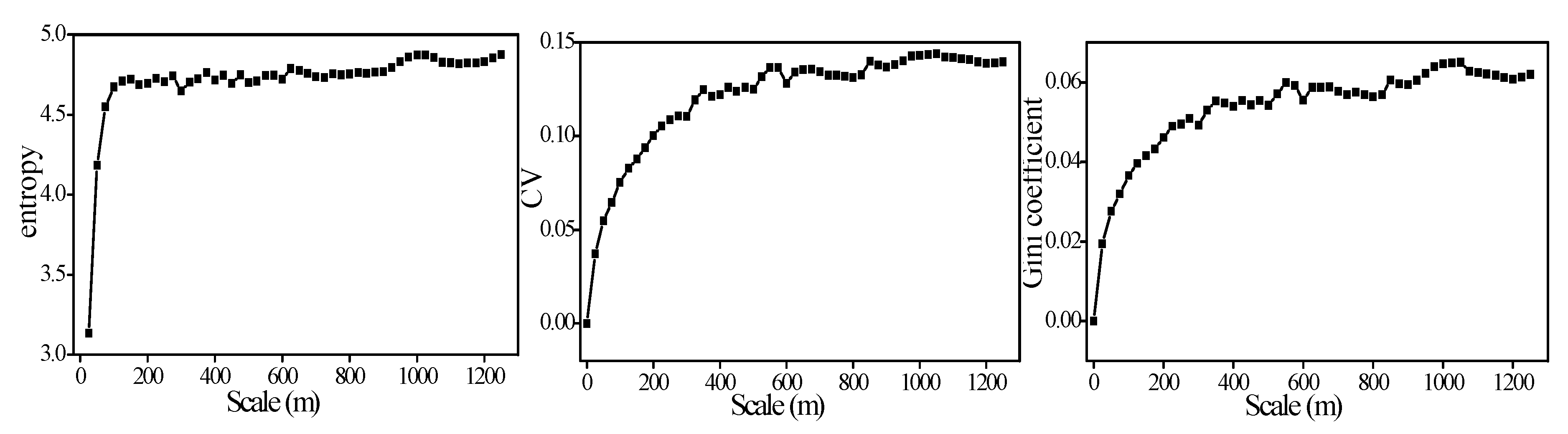
Figure 8.
Temporal variation of the entropy and CV of surface variables (i.e., H, LE and Ts_0cm).


Table 1.
Calculation results of the three methods for the simulated data in Scheme 1.
| Distribution Type | Specific Parameters | S | CV | Gini |
|---|---|---|---|---|
| Normal | N(1) u = 0.5, sd = 0.12 | 3.8596 | 0.2311 | 0.1305 |
| N(2) u = 0.5, sd = 0.09 | 3.5437 | 0.1685 | 0.0950 | |
| N(3) u = 3, sd = 0.30 | 4.7925 | 0.0986 | 0.0557 | |
| Beta | B(1) α = 6, β = 1 | 5.0479 | 0.1445 | 0.0771 |
| B(2) α = 1, β = 6 | 5.0478 | 0.8697 | 0.4638 | |
| B(3) α = 0.5, β = 0.5 | 5.7996 | 0.7081 | 0.4057 | |
| Gamma | G(1) k = 1, θ = 2 | 4.3049 | 0.9901 | 0.4965 |
| G(2) k = 2, θ = 2 | 4.8676 | 0.7066 | 0.3756 | |
| G(3) k = 3, θ = 2 | 5.1169 | 0.5777 | 0.3126 | |
| G(4) k = 1, θ = 5 | 3.3721 | 0.9291 | 0.4848 | |
| Weibull | W(1) k = 5, λ = 0.5 | 2.9733 | 0.2262 | 0.1278 |
| W(2) k = 1, λ = 1 | 4.8165 | 0.9824 | 0.4947 | |
| W(3) k = 15, λ = 1 | 2.6494 | 0.0807 | 0.0446 | |
| Exponential | E(1) λ = 1 | 4.7244 | 1.0090 | 0.5011 |
| E(2) λ = 4 | 3.3821 | 0.9968 | 0.4975 | |
| E(3) λ = 8 | 2.7327 | 0.9941 | 0.5005 | |
| Uniform | U(1) min = 0, max = 1 | 3.7550 | 0.5779 | 0.3336 |
| U(2) min = 0, max = 10 | 5.9966 | 0.5734 | 0.3310 |
Note: u represents the mean; sd represents the standard deviation; s represents the entropy value; in the same distribution, the interval division of entropy is consistent.
Table 2.
Calculation results of the three methods for the simulated data in Scheme 2.
| Distribution Type | Specific Parameters | S | CV | Gini |
|---|---|---|---|---|
| Normal | (a) u = 0.5, sd = 0.12 | 5.2604 | 0.2311 | 0.1305 |
| (b) u = 0.5, sd = 0.09 | 4.9459 | 0.1685 | 0.0950 | |
| Beta | (c) α = 6, β = 1 | 5.0479 | 0.1445 | 0.0771 |
| (d) α = 1, β = 6 | 5.0478 | 0.8697 | 0.4638 | |
| (e) α = 0.5, β = 0.5 | 5.8003 | 0.7081 | 0.4057 | |
| Gamma | (f) k = 1, θ = 5 | 5.3579 | 0.9291 | 0.4848 |
| Weibull | (g) k = 5, λ = 0.5 | 5.1505 | 0.2262 | 0.1278 |
| Exponential | (h) λ = 8 | 4.9230 | 0.9941 | 0.5005 |
| Uniform | (i) min = 0, max = 1 | 5.9984 | 0.5779 | 0.3336 |
Note: u represents the mean; sd represents the standard deviation; s represents the entropy value.
Table 3.
Calculation results of the three methods for the simulated data in Scheme 3.
| Distribution Type | Specific Parameters | S | CV | Gini |
|---|---|---|---|---|
| Normal | (a) u = 1.5, sd = 0.12 | 5.2604 | 0.0771 | 0.0435 |
| (b) u = 1.5, sd = 0.09 | 4.9459 | 0.0561 | 0.0316 | |
| Beta | (c) α = 6, β = 1 | 5.0479 | 0.0667 | 0.0356 |
| (d) α = 1, β = 6 | 5.0478 | 0.1085 | 0.0578 | |
| (e) α = 0.5, β = 0.5 | 5.8003 | 0.2361 | 0.1353 | |
| Gamma | (f) k = 1, θ = 5 | 5.3579 | 0.1516 | 0.0791 |
| Weibull | (g) k = 5, λ = 0.5 | 5.1505 | 0.0713 | 0.0403 |
| Exponential | (h) λ = 8 | 4.9230 | 0.1103 | 0.0556 |
| Uniform | (i) min = 1, max = 2 | 5.9984 | 0.1924 | 0.1111 |
Note: u represents the mean; sd represents the standard deviation; s represents the entropy value; (c–h) are obtained by shifting one unit to the right on the basis of the Scheme 2.
Table 4.
Calculation results of the three methods for each variable in different areas.
| Track NO. | Area NO. | S | CV | Gini | Track NO. | Area NO. | S | CV | Gini | ||||||
|---|---|---|---|---|---|---|---|---|---|---|---|---|---|---|---|
| LAI | LST | LAI | LST | LAI | LST | LAI | LST | LAI | LST | LAI | LST | ||||
| track 5-1 | 1 | 5.3350 | 4.4594 | 0.4050 | 0.1303 | 0.2114 | 0.0545 | track 10-1 | 10 | 5.3660 | 4.2306 | 0.4715 | 0.1329 | 0.2478 | 0.0574 |
| 2 | 5.3209 | 4.5029 | 0.4427 | 0.1389 | 0.2334 | 0.0604 | 11 | 5.3818 | 4.0387 | 0.4022 | 0.1023 | 0.2093 | 0.0401 | ||
| 3 | 5.3494 | 4.6007 | 0.5692 | 0.1494 | 0.3128 | 0.0708 | 12 | 5.5580 | 4.3174 | 0.4653 | 0.1106 | 0.2528 | 0.0473 | ||
| track 5-2 | 4 | 5.3034 | 4.5020 | 0.4014 | 0.1288 | 0.2080 | 0.0543 | track 11-1 | 13 | 5.5324 | 4.3848 | 0.5158 | 0.1292 | 0.2814 | 0.0571 |
| 5 | 5.3407 | 4.5748 | 0.4309 | 0.1347 | 0.2268 | 0.0591 | 14 | 5.5262 | 3.9989 | 0.3937 | 0.0968 | 0.2065 | 0.0383 | ||
| 6 | 5.3939 | 4.5033 | 0.5083 | 0.1410 | 0.2750 | 0.0632 | 15 | 5.5739 | 4.1628 | 0.4020 | 0.0997 | 0.2120 | 0.0402 | ||
| track 7-2 | 7 | 5.3480 | 4.1616 | 0.3737 | 0.1140 | 0.1925 | 0.0434 | track 12-1 | 16 | 4.8339 | 4.4876 | 0.7941 | 0.1176 | 0.4462 | 0.0523 |
| 8 | 5.3573 | 4.3790 | 0.4258 | 0.1196 | 0.2240 | 0.0508 | 17 | 4.7221 | 4.1904 | 0.7181 | 0.0868 | 0.3955 | 0.0362 | ||
| 9 | 5.4848 | 4.5773 | 0.5030 | 0.1357 | 0.2751 | 0.0667 | 18 | 4.8323 | 4.3546 | 0.6973 | 0.1084 | 0.3830 | 0.0480 | ||
Table 5.
The number of observations in the calculation of each variable.
| Variable | Number of Observation | Variable | Number of Observation | Variable | Number of Observation |
|---|---|---|---|---|---|
| H | 17 | RH_5m | 17 | albedo | 16 |
| LE | 17 | Ta_5m | 17 | Rn | 16 |
| Ustar | 17 | Ms_2cm | 17 | Ts_0cm | 17 |
Note: H represents sensible heat flux; LE represents latent heat flux; Ustar represents the friction wind speed which is observed by an ultrasonic anemometer; RH_5m represents air humidity at 5 m; Ta_5m represents air temperature at 5 m; Ms_2cm represents soil moisture at a depth of 2 cm; albedo represents the surface albedo, which is obtained by the ratio of the upward shortwave radiation to the downward shortwave radiation; Rn represents net radiation; Ts_0cm represents soil temperature at a depth of 0 cm (i.e., the temperature measured by the detector exposed to the Earth’s surface).
Table 6.
Statistics of the entropy for each variable.
| Variable | MIN | MAX | MEAN | STD |
|---|---|---|---|---|
| H | 0.649 | 1.000 | 0.913 | 0.061 |
| LE | 0.747 | 1.000 | 0.929 | 0.048 |
| Ustar | 0.798 | 1.000 | 0.946 | 0.036 |
| RH_5m | 0.748 | 1.000 | 0.923 | 0.041 |
| Ta_5m | 0.693 | 1.000 | 0.875 | 0.050 |
| Ms_2cm | 0.863 | 1.000 | 0.982 | 0.024 |
| albedo | 0.670 | 1.000 | 0.919 | 0.049 |
| Rn | 0.423 | 1.000 | 0.918 | 0.056 |
| Ts_0cm | 0.769 | 1.000 | 0.932 | 0.048 |
© 2018 by the authors. Licensee MDPI, Basel, Switzerland. This article is an open access article distributed under the terms and conditions of the Creative Commons Attribution (CC BY) license (http://creativecommons.org/licenses/by/4.0/).
Share and Cite
MDPI and ACS Style
Li, X.; Xin, X.; Peng, Z.; Zhang, H.; Yi, C.; Li, B. Analysis of the Spatial Variability of Land Surface Variables for ET Estimation: Case Study in HiWATER Campaign. Remote Sens. 2018, 10, 91. https://doi.org/10.3390/rs10010091
AMA Style
Li X, Xin X, Peng Z, Zhang H, Yi C, Li B. Analysis of the Spatial Variability of Land Surface Variables for ET Estimation: Case Study in HiWATER Campaign. Remote Sensing. 2018; 10(1):91. https://doi.org/10.3390/rs10010091
Chicago/Turabian StyleLi, Xiaojun, Xiaozhou Xin, Zhiqing Peng, Hailong Zhang, Chuanxiang Yi, and Bin Li. 2018. "Analysis of the Spatial Variability of Land Surface Variables for ET Estimation: Case Study in HiWATER Campaign" Remote Sensing 10, no. 1: 91. https://doi.org/10.3390/rs10010091
Note that from the first issue of 2016, this journal uses article numbers instead of page numbers. See further details here.