Adaptive Window-Based Constrained Energy Minimization for Detection of Newly Grown Tree Leaves


1
Department of Computer Science and Information Engineering, National Yunlin University of Science and Technology, Douliu 64002, Taiwan
2
Department of Forestry and Natural Resources, National Chiayi University, Chiayi 60004, Taiwan
*
Author to whom correspondence should be addressed.
Remote Sens. 2018, 10(1), 96; https://doi.org/10.3390/rs10010096
Submission received: 23 November 2017
/
Revised: 23 December 2017
/
Accepted: 8 January 2018
/
Published: 12 January 2018
(This article belongs to the Special Issue Hyperspectral Imaging and Applications)
Abstract
:Leaf maturation from initiation to senescence is a phenological event of plants that results from the influences of temperature and water availability on physiological activities during a life cycle. Detection of newly grown leaves (NGL) is therefore useful for the diagnosis of tree growth, tree stress, and even climatic change. This paper applies Constrained Energy Minimization (CEM), which is a hyperspectral target detection technique to spot grown leaves in a UAV multispectral image. According to the proportion of NGL in different regions, this paper proposes three innovative CEM based detectors: Subset CEM, Sliding Window-based CEM (SW CEM), and Adaptive Sliding Window-based CEM (AWS CEM). AWS CEM can especially adjust the window size according to the proportion of NGL around the current pixel. The results show that AWS CEM improves the accuracy of NGL detection and also reduces the false alarm rate. In addition, the results of the supervised target detection depend on the appropriate signature. In this case, we propose the Optimal Signature Generation Process (OSGP) to extract the optimal signature. The experimental results illustrate that OSGP can effectively improve the stability and the detection rate.

1. Introduction
The persistence of forest ecosystem resources is the key to protecting wild coverage of reproductive trees in order to alleviate global warming or the impact of climate change. Specifically, the variance in the area of woods, the accumulation of forest biomass/carbon storage, and the improvement of healthy forests are the periodic evaluation indices of global forest resources for forest sustainability, according to Forest Resources Assessment FAO (Food and Agriculture Organization of the United Nations) [1]. Therefore, using telemetry to monitor the health level of forest ecosystems has a critical effect on the subject of global warming control. Climate change may affect phenological events such as the onset of green-up and dormancy [2]. Trees start to sprout once they sense the growing signals in early spring. After the leaf initiation stage, the newly sprouted leaflet will gradually develop and further facilitate tree growth in crown width, height, diameter, and carbon storage [3]. As a result, the newly grown leaves (NGL) can be seen as the first objects of trees in response to a change in temperature, and can therefore provide critical information for the early detection of climate changes [4]. UAV-sensed images are generally collected at low altitude; the images are supposedly free of atmospheric effects [5], and provide very high spatial resolution for applications. Taking the strengths of UAV-sensed images, NGL over a forest area can be detected via appropriate remote sensing techniques.
In forest science, remote sensing has been applied to investigate species classification [6,7], tree delineation [8,9], and biomass productivity estimation [10,11]. The detection of NGL is a new application in respect to the previous applications. The target of interest may occur under a very low probability or probably has a relatively smaller size than the background, such as the damaged portion of crown in the forest canopy or the new leaf crown in the forest canopy. In this case, the traditional spatial domain (i.e., literal)-based image processing techniques [12,13,14,15] may fail to extract these targets effectively, especially when the target size is smaller than the pixel resolution. In contrast, the technique using spectral characteristics to detect the subpixel level is one of the more feasible methods. From the angle of multispectral/hyperspectral detection, the spectral information-based target detection technique [16,17,18] should be able to solve these problems.
Hyperspectral subpixel detection techniques can be divided into active and passive manners. In the active methods, the detectors only use single or multiple spectral signatures of targets of interest for detection purposes; e.g., Constrained Energy Minimization (CEM) [19], Correlation Mahalanobis Distance (RMD) [7,20], Mahalanobis Distance (KMD) [17,21], Adaptive Coherence Estimator (ACE) [22], Target-Constrained Interference-Minimized Filter (TCIMF) [17,18,23], etc. The correctness of target information plays an important role. Incorrect information results in a false alarm and omission of a target detection result. Therefore, how to provide the correct target object information is a very important step. The Optimal Signature Generation Process (OSGP) that is proposed in this paper increases the accuracy of selecting a target iteratively so as to solve the previously mentioned problem.
Hyperspectral algorithms have been developed for many different target detections in recent years and are used in different areas [24,25,26,27,28,29]. Many studies have proposed CEM based algorithms [30,31] in the last decade. However, using hyperspectral algorithms to detect targets in RGB images presents several issues since spectral information is insufficient and spatial information is not used, and thus a false alarm is likely to occur where there is a similar spectral characteristic. In order to solve this dilemma, this paper proposes three innovative CEM based detectors-Subset CEM, Sliding Window-based CEM, and Adaptive Sliding Window-based CEM to establish their own autocorrelation matrix, and uses sliding window point-to-point scanning for calculation. As the sliding window passes through, the contrast between a NGL and the background can be enhanced. When compared with traditional CEM results that incur too many false alarms, our proposed methods can solve this issue and produce more stable results.
2. Materials and Methods
2.1. Constrained Energy Minimization
Traditional Constrained Energy Minimization (CEM) [16,17,18,19] of active hyperspectral target detection is the major technique that is adopted in this paper. The CEM only needs the spectral signature of one specific target of interest during target detection; it is free of the spectral signature of other targets or background. Many target detection methods have been proposed in recent years, among those, the CEM only needs the signature of one target of interest and the detection is stable. Thus, this paper selects CEM to compare local improvement methods. In the CEM algorithm, only one spectral signature (desired signature or target of interest) is given, referred to as d, any prior knowledge is not required, e.g., multiple targets of interest or background. In other words, users can extract the specific target of interest without any background information, implementing target detection. This is one of the major advantages of CEM. Another advantage of CEM is that as many signal sources cannot be recognized or observed with the naked eye, some materials may be detected by sensors leading to false alarm. However, the CEM transposes the correlation matrix R of data samples before the desired signature d is extracted. The sample autocorrelation matrix can be defined as , so that the background can be suppressed by R, and the filter is matched with signature d to enhance the capability of detecting signature, the execution is more efficient. The CEM is evolved from the LCMV proposed by Frost [32]. If there are N pixels in a hyperspectral image with L band, which are , where , the desired target to be looked for is represented by d, defined as , the desired target to be looked for can be detected by finite impulse response filter (FIR) based on CEM and desired target d. The filter coefficient is defined as , the w can be obtained with the minimum average energy, defined as . Therefore, if is defined as and imported into FIR, and then can be expressed as
The average energy is
With the minimum average energy, the optimal solution of w can be obtained
According to the theory of Harsanyi [19], the optimal solution to the weight vector of one L band is
Equation (3) is substituted in Equation (2), the result of CEM is
2.2. Subset CEM
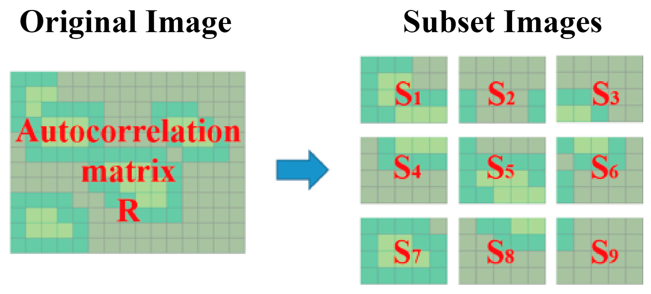
The first target detection algorithm using autocorrelation matrix S that is proposed in this paper is a novel method using subsets, known as Subset CEM. The Subset CEM splits the image into several small square images; these small images are the subsets of the original image. The CEM detection is then implemented, and the results of subsets are patched up to obtain a complete resulting image. In other words, the small image of each subset has its own autocorrelation matrix S. For example, a 1200 × 1500 image is divided into nine small images; the resolution of each small image is 400 × 500, the autocorrelation matrix S is S1, S2, S3, …, S9, respectively, and the corresponding Sn of each pixel is substituted into CEM for detection, thus obtaining the result. Figure 1 is the schematic diagram of the autocorrelation matrix in the image. The subset image size of the local autocorrelation matrix S is obtained by trial and error. Normally, using five times smaller than the original size is a good first try. The image resolution used in this paper is 1000 × 1300, and thus the image is divided into 200 × 260 subset images.
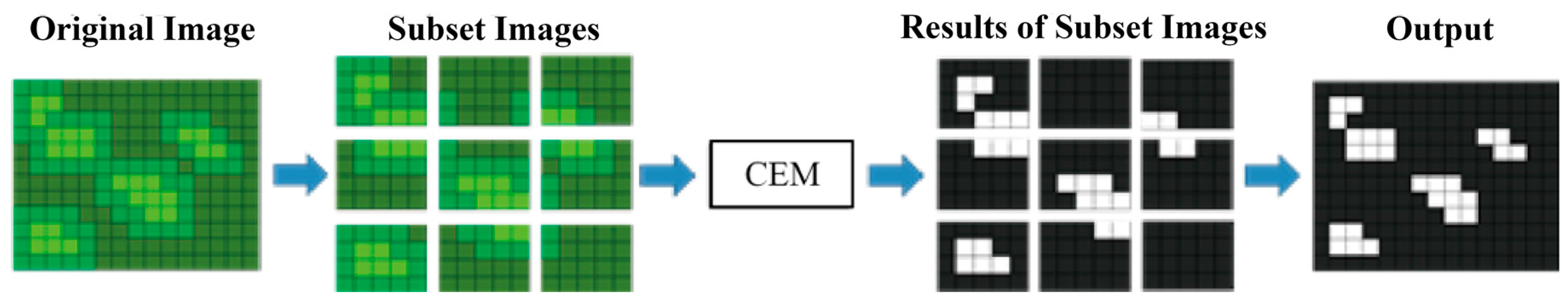
The results show that this method can effectively suppress the background pixels that are too similar to the desired target. Because the image is divided into the set of small images, the autocorrelation matrix of each small image changes accordingly. There is a different S for suppressing the background according to different images, and S is calculated according to the pixels in a small area; thus, the small difference between similar spectral signatures is enlarged. It is easier to judge the difference between two RGB values for suppression, so as to increase the detection rate. Figure 2 shows the detection process after the Subset CEM splits the image into subsets.
2.3. Sliding Window-Based CEM (SW CEM)
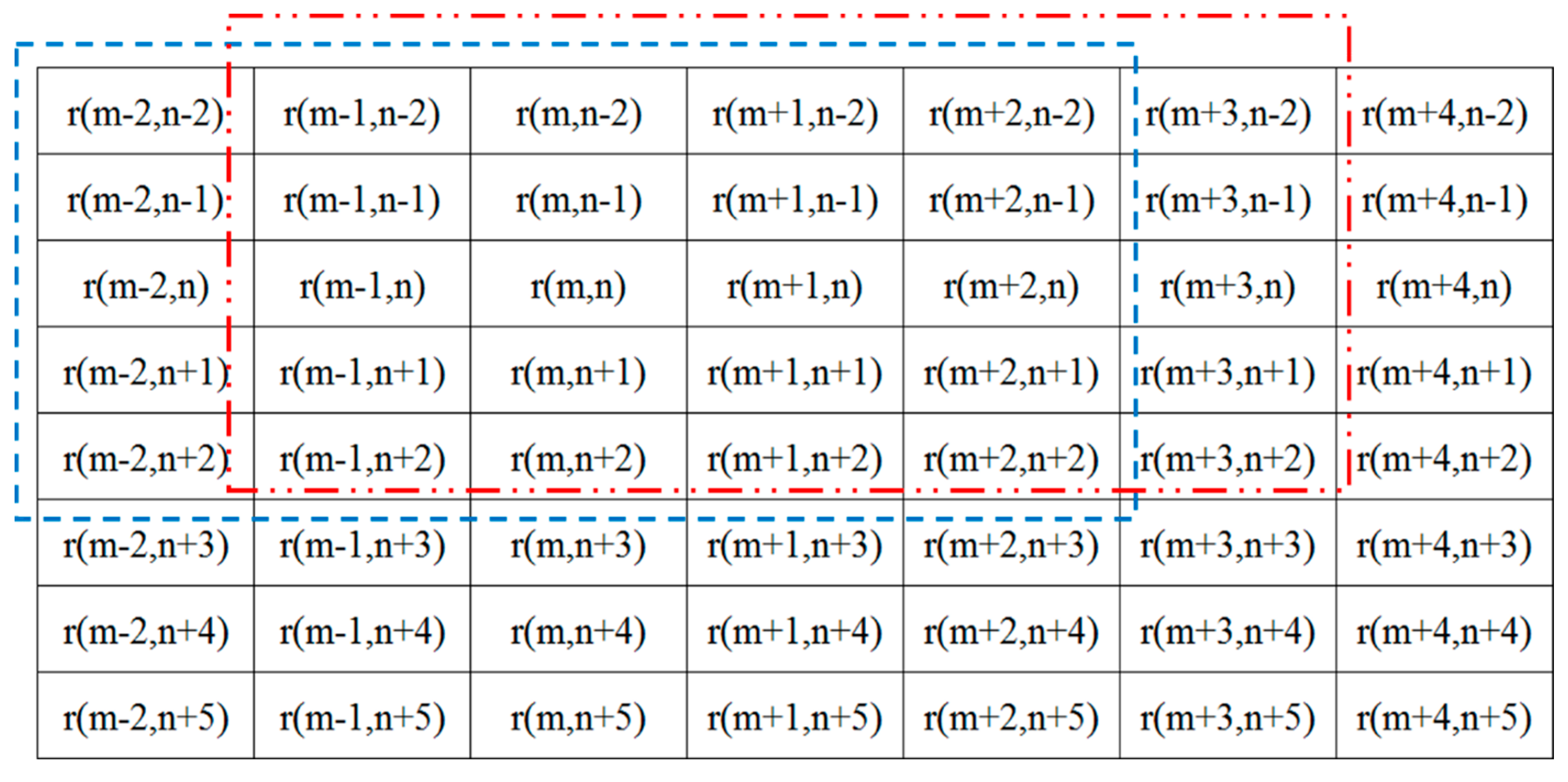
Section 2.2 mentioned that the Subset CEM can effectively reduce the false alarm rate of similar background spectrums using the concept of the local autocorrelation matrix S. The Subset CEM divides the image into small square images, where each small image has its own autocorrelation matrix S. In other words, every two small images have dissimilar S. However, Subset CEM uses non-overlapped windows, which causes artifacts at the borders of subset images. In order to resolve such an issue, this paper proposes the pixel-by-pixel sliding window-based CEM (SW CEM) for detection. The sliding window concept is used in many studies [27,33,34,35]. The pixel-by-pixel CEM uses a sliding window of fixed size to obtain the RGB values around each pixel, according to different spectral characteristics around each pixel, so as to determine its autocorrelation matrix Sn. In other words, if the Subset CEM divides the image into small square images, then the pixel-by-pixel CEM divides the image into pixels, combined with a sliding window, to acquire the pixels around the pixel to determine the autocorrelation matrix Sn. Figure 3 shows the sliding window and direction.
This means that each pixel in the image has its Sn, and each Sn is independent and different. Hence, the SW CEM can be defined as:
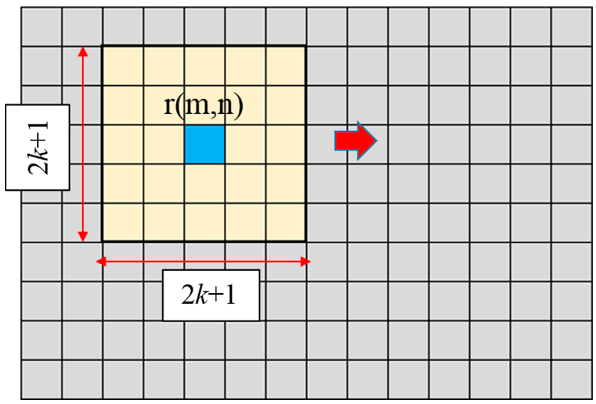
where, is the current pixel value, and is the autocorrelation matrix of , if the size of the sliding window is 2k + 1, as shown in Figure 4.
When the size of a sliding window is known, can be defined as:
where, represents each pixel in the sliding window, and is a constant, if is simplified by .
We substitute Equation (8) into Equation (6) to obtain:
where, is the autocorrelation matrix of current pixel , and the capability of suppressing the background can be enhanced for each region by .
2.4. Adaptive Sliding Window-Based CEM (ASW CEM)
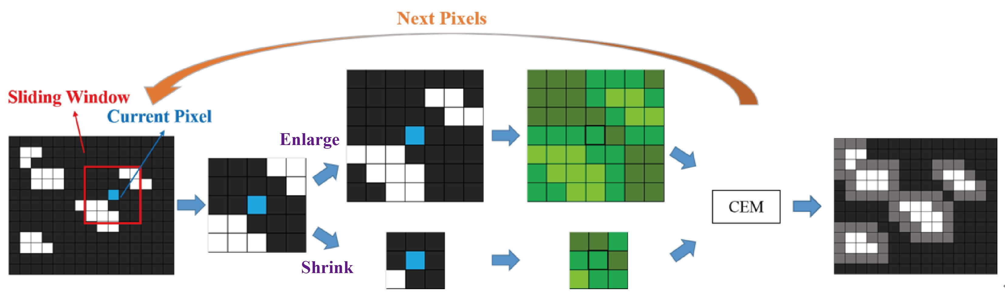
The adaptive window concept has been applied to targets detection in many applications in the last decade, such as vehicles detection [36,37], adaptive filters [38], and anomaly detection [39,40]. When compared to SW CEM, which uses a fixed window size to calculate autocorrelation matrices S, AWS CEM determines the window size according to the spatial and spectral characteristics around each pixel, so as to suppress the background. The optimum size of the sliding window varies with the quantity of NGL around each pixel, and thus the sliding window improves based on the local CEM in this paper. The size of sliding window is determined by acquiring the proportion of sprouts around the current pixel. When the sliding window size 2K + 1 of the current pixel is determined, the result of SW CEM target detection can be obtained. In this case, we developed Adaptive Sliding Window-based CEM (ASW CEM) to combine adaptive window concept in CEM. Figure 5 illustrates the flowchart of ASW CEM. ASW CEM can change the size of the sliding window according to the ratio of the NGL around the current pixel to enhance NGL and suppress background.
The execution of ASW CEM comprises six steps:
- Input image
- Decide the default size of the sliding window
- Calculate the rate of the sprout in the sliding window
- If the rate of the sprout meets the set condition or the window size has reached the default maximum or minimum window, then the S in Equation (10) is calculated according to the pixel values of the current window size. If the rate of the sprout is not met or the window size has not reached the limit value, then the size of the sliding window is changed and return to Step 3; otherwise, proceed to Step 5.
- The S obtained in Step 4 is used to calculate CEM to obtain the result value of the current pixel.
- If all pixels of the image have been calculated, then ASW CEM detection is finished; otherwise, return to Step 2.
The calculation of the rate of the sprout in the sliding window in Step 3 and the sliding window change conditions in Steps 2 and 4 are introduced below.
2.4.1. Acquire the Rate of the NGL around the Current Pixel (NGL Map)
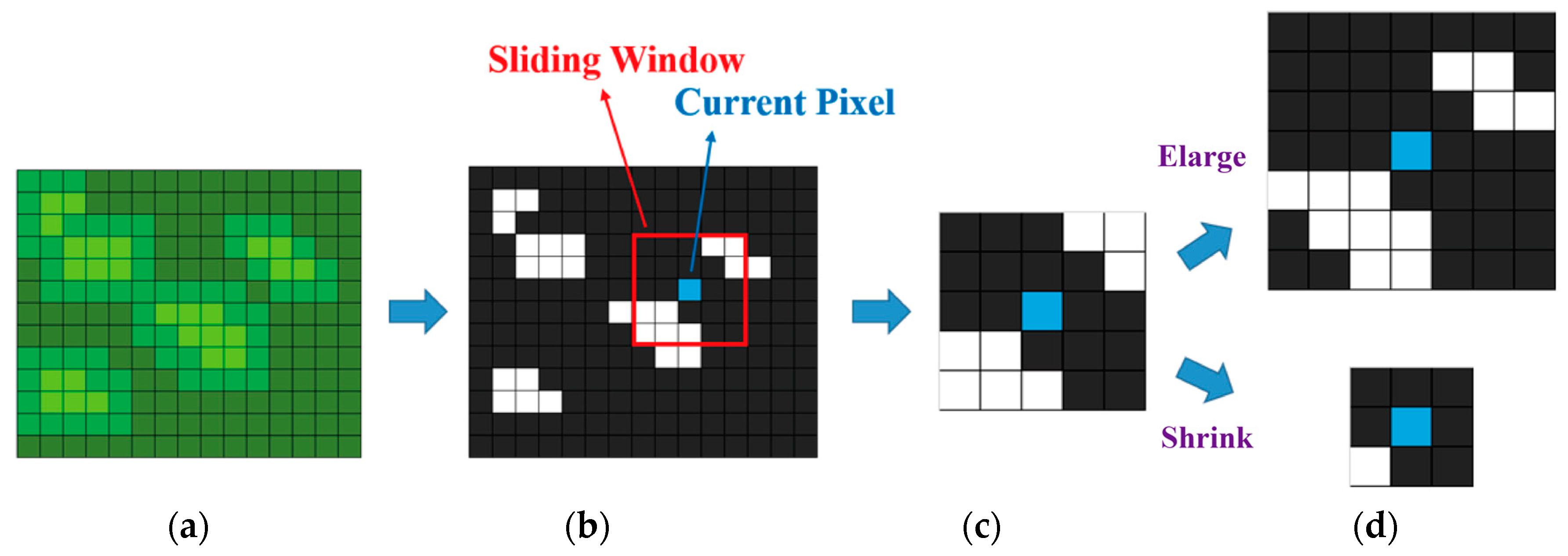
In order to enable the sliding window of each pixel to decide whether or not to enlarge or to shrink the current window according to the proportion of peripheral NGL, this paper requires a sprout map for judgment and reading. To set up the sprout distribution map, the spectral comparison is conducted on the he Spectral Information Divergence (SID) [17,41] for experimental multispectral images before ASW CEM, so as to obtain a preliminary sprout detection result. This result contains a small false alarm, but according to this result, when deciding whether or not to enlarge or shrink the sliding window, only the relative rate of the sprout in the sliding window shall be calculated, as the actual number of NGL is not required. The SID resulting image is segmented several times by using Otsu’s method [42]. The rate of the sprout in the image is preliminarily estimated at 1~2%, so as to minimize the false alarm, and the major sprout points are maintained for calculation. When the image with a preliminary estimate of the sprout is obtained, the proportion of NGL can be calculated by using the default sliding window size, and the size of the sliding window is changed according to the number of NGL. Figure 6 is the flowchart of this step.
2.4.2. Adaptive Sliding Window
To calculate the rate of the sprout around the current pixel, a sliding window of preset size needs to be made. The rate of the sprout in this window decides whether or not to enlarge or shrink the sliding window for subsequent algorithmic detection. Figure 7 is the flowchart of this step. A larger sliding window size is required in the region with a higher rate of the sprout; the optimum size of maximum window is set as m2; on the contrary, a smaller sliding window size is required in the region with a lower rate of the sprout, and the optimum size of the smallest window is set as n2. When the maximum window m2 and minimum window n2 are obtained, the default window is set as an intermediate between maximum and minimum windows, i.e., . The advantage is that as the initial window is intermediately sized, the window is enlarged or shrunk to the limit relatively fast. Afterwards, the sliding window is enlarged or shrunk gradually, according to the rate of the sprout in the window.
As the distribution of NGL is not even, when the window is shrunk or enlarged, the rate of the sprout does not always increase or decrease. This method can enlarge and shrink the window. In order to avoid the non-uniform rate of the sprout leading to an infinite circulation of window enlargement or shrinkage, the initial window is used to calculate the sprout as a watershed. When the rate of the sprout in the initial window is higher than a threshold, the sliding window is enlarged gradually until the rate of the sprout in the window is lower than a threshold or the window is maximized before CEM detection. If the rate of the sprout in the initial window is lower than a threshold, then the sliding window is shrunk gradually until the rate of the sprout in the window is higher than a threshold, or the window is minimized before CEM detection. In order to adjust the window size conditionally in the stable level, this paper includes a parameter ε as initial NGL rate in the window, where ε is the proportion of the number of NGL in the window to the total number of pixels in the sliding window. When the rate of the sprout in the window is lower than ε, the window is shrunk; if the rate of the sprout in the window is higher than ε, then the window is enlarged.
2.5. Optimal Signature Generation Process (OSGP)
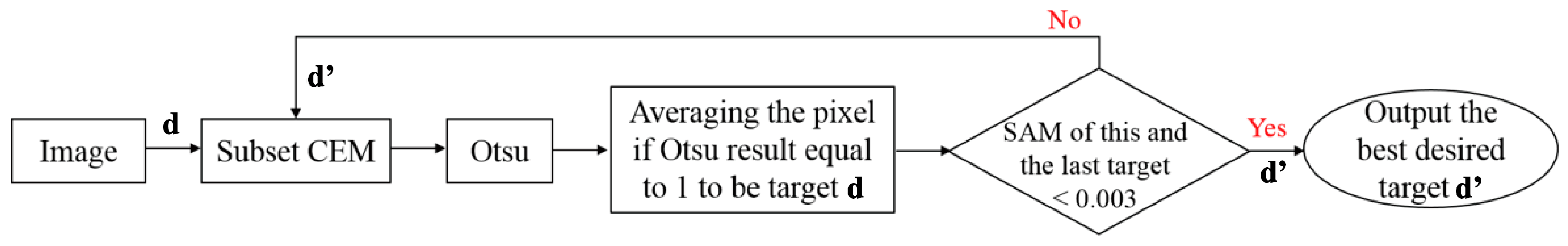
In order to remedy the defect in the CEM-related algorithm in that only one desired target can be selected, the Optimal Signature Generation Process (OSGP) is used herein to obtain a stable desired target by the iterative process. The idea of the iterative process is similar to K-means [43], iterative self-organizing data (ISODATA) [44] and iterative FLDA [45]. The OSGP implements Subset CEM target detection for the image iteratively. When the result of CEM is obtained, the image is segmented by using Otsu’s method until the number of result pixels is 2–3%, which is the target pixel with the highest probability of the sprout. These pixels correspond to the same pixel RGB values in the original image, averaged as a new target d’. If the pixel value of d’ is not similar enough to that of d, then d’ is substituted in the next CEM, a new desired target is obtained. This is repeated until this and the last Spectral Angle Mapper [46] are smaller than a value θ, and then the current target d is exported. The threshold of spectral angle was tested continuously, and the threshold was set as 0.003. Figure 8 is the flowchart of OSGP.
It is noteworthy that CEM uses the global correlation matrix R to suppress the background, and it is likely that the background has similar spectral signatures. Simply iterating CEM is the same condition, and some background pixels that do not belong to the desired target will be misrecognized as the result pixels, and the averaging of them influences the new desired target. A stable target d is still obtained after iteration, but the misrecognized pixels may result in errors in d, thus reducing the detection accuracy slightly. To solve this dilemma, this paper proposes Optimal Signature Generation Process (OSGP) and replaces CEM by subset CEM. The Subset CEM splits the image into many small sets; in the global view of the full image, the small square image of a subset is the local concept. The local algorithm can effectively suppress the pixel RGB values similar to the desired target, which is substituted into the iterative algorithm. This not only reduces the misrecognized result of pixels during iteration, but also obtains a better desired target d, so that the precision of detection increases and the probability of a false alarm decreases.
2.6. Parameter Settings of Different Algorithms
For different parameter settings of algorithms in this paper, the results are different, and so the parameter settings of the multiple CEM algorithm are listed in this section, as shown in Table 1. The input d of CEM, Subset CEM, SW CEM, and ASW CEM is the randomly selected desired target. The desired target d’ is iterated by using OSGP. The OSGP iteration stop condition is that the SAM value of two adjacent targets d shall be smaller than θ; if tenable, then the desired target d’ is exported. Here, ε is the condition value of the rate of the sprout when the sliding window of ASW CEM is enlarged or shrunk. In the following experiments in this study, ε is set to 1%. However, this parameter depends on the proportion of the number of target pixel in the entire image.
In the following experiments the Subset image size is set as 200 × 260 pixel, and each small image uses the same d and d’, where each small image takes the pixels of its image size to calculate S. The subset image size of the local autocorrelation matrix S is obtained by trial and error. When each small image has calculated CEM, the results are exported and merged into the original picture size, and the merged picture is the result of Subset CEM.
The window size of SW CEM varied by different application and images. Normally, 5–6 times smaller than the entire images are the good try as the initial setting. This study sets the sliding window size as 151 × 151 pixel. It extracts the pixels of 151 × 151 pixel around each pixel to calculate S in Equation (10), which are substituted into CEM in order to work out the result value of the pixel. When each pixel is calculated, the output result of SW CEM is obtained.
ASW CEM uses the original image for SID measurement and gives the preliminarily estimated NGL map, and then ASW CEM employs the sliding window of preset size to calculate the rate of the sprout. When the rate of the sprout mismatches the stop condition, the window size is changed and this rate in the window is recalculated, until the window size reaches the threshold or the rate of the sprout is equivalent to ε. The pixel values in this window are used to calculate S, which is substituted into CEM to work out the result value of the pixel. When each pixel has been calculated, the output result of ASW CEM is obtained. For this experiment, the maximum size of the sliding window is set as 151 × 151, the minimum window is 31 × 31, and the initial window is 91 × 91. The initial window size can be set as the average of the maximum and minimum size.
3. Experiments
3.1. Experimental Procedure
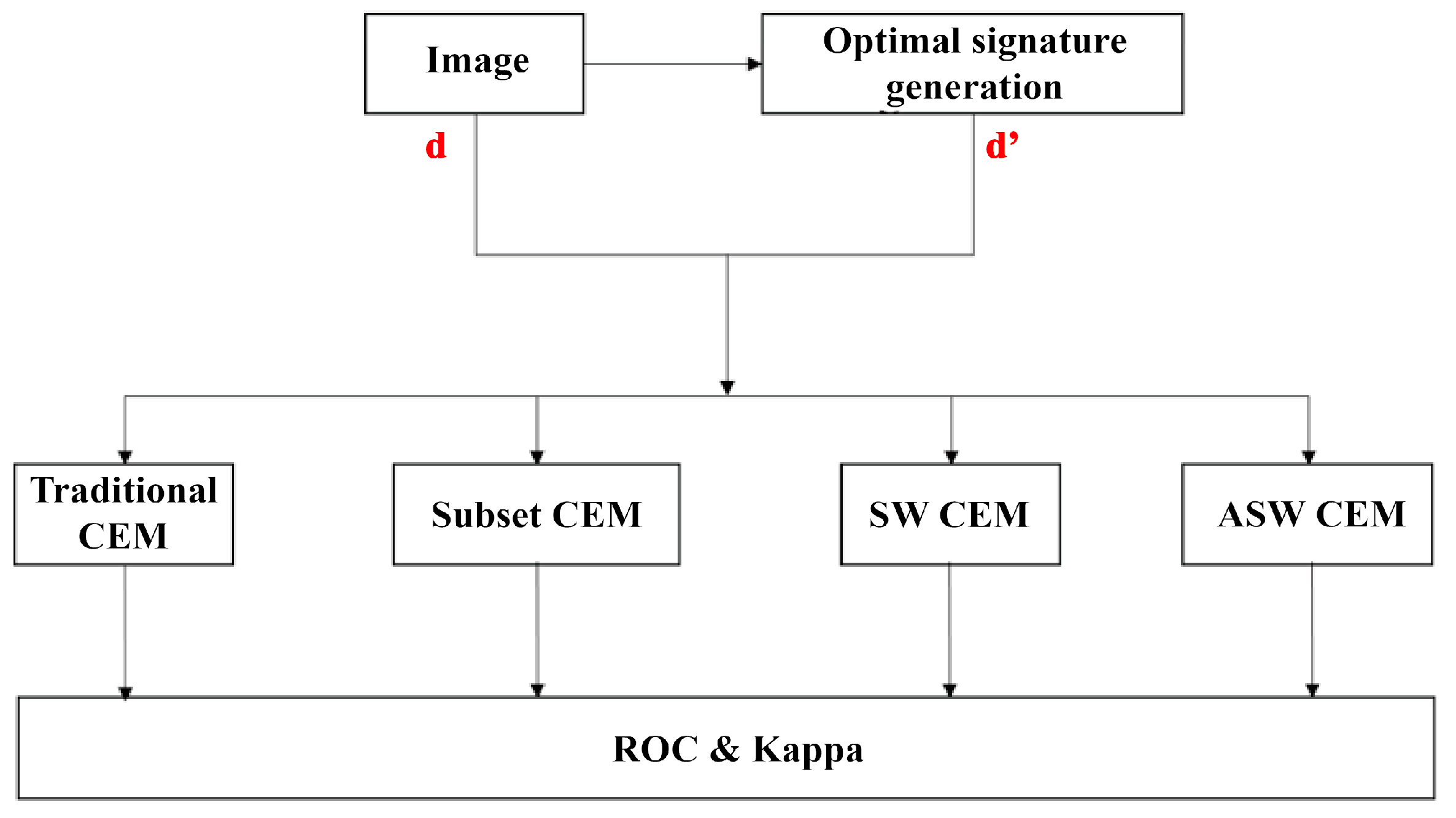
This section introduces the experimental process of all detection algorithms used in this paper, including CEM, Subset CEM, Sliding Window-based CEM, and Adaptive Sliding Window-based CEM. In order to remedy the defect in the target detection algorithm that only one d can be selected at one time, the Optimal Signature Generation Process (OSGP) is used, and the optimum target of interest d’ is iterated by iterative learning. The incorrect results of selection errors are thus reduced effectively. Figure 9 shows the approximate process of all the detection algorithms for this experiment.
There are two methods of hyperspectral target detection for selecting the desired target. One method only selects the single target d for detection. The other method selects the pixel values of multiple desired targets for detection. The CEM is the first type. CEM only selects a single target for detection, and so the quality of detection result highly depends on the selected desired target.
The desired targets d used by all of the detection algorithms for the experiments are randomly selected from the ground truth and d’ is iterated by using OSGP to increase the precision of detection. The full image is used to calculate autocorrelation global R for target detection of CEM.
3.2. Description of the Study Site
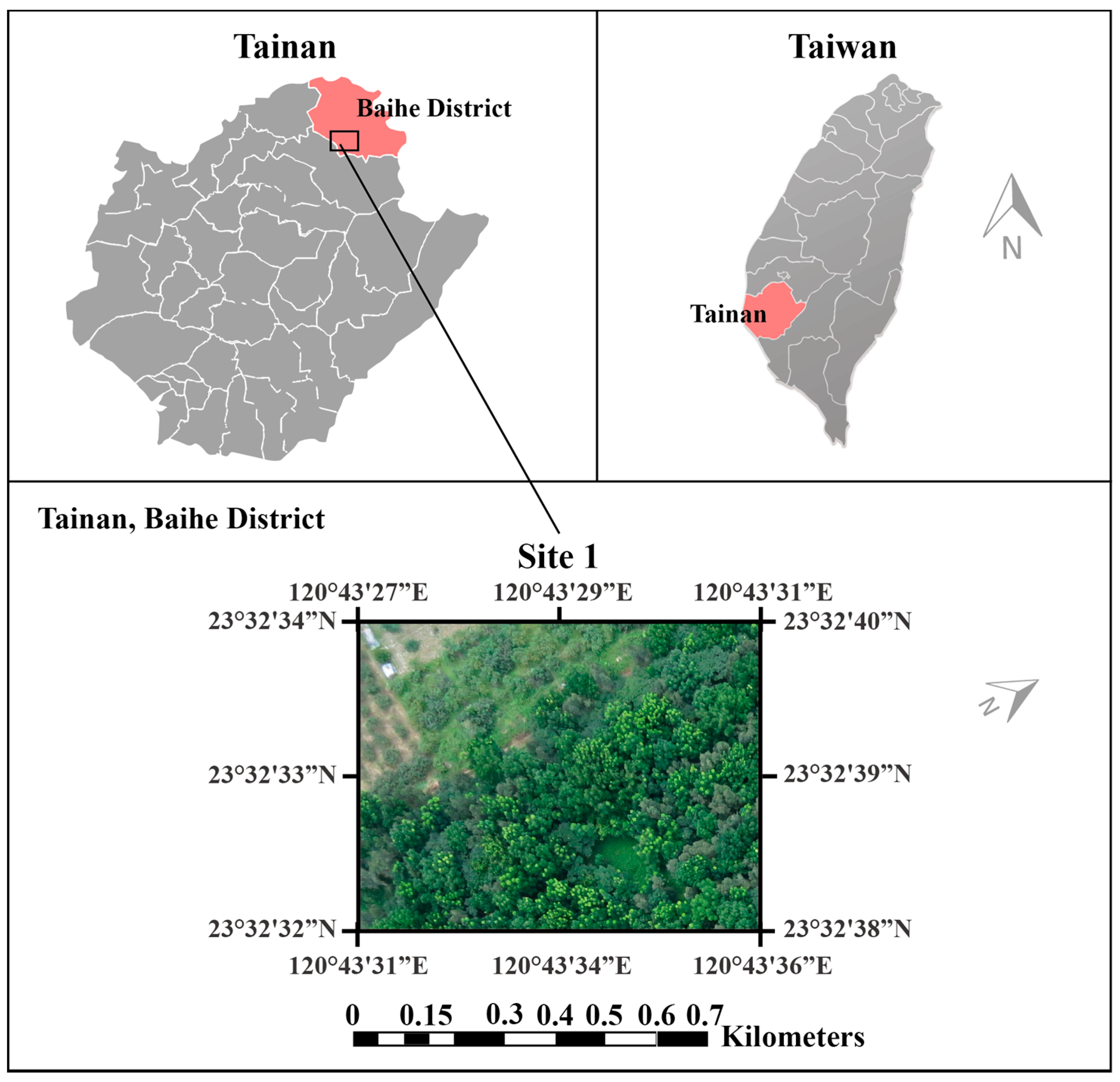
The study site is in Baihe District (23°20′N, 120°27′E) which is part of Tainan City, Taiwan. Tainan City is characterized by a tropical savanna climate. The weather is generally hot and humid. The mean annual temperature is 24.38 °C. The authors have deployed a few permanent plots over the broadleaf forest for research of forest growth [47,48] in 2008. In which, a series of ground inventory is annually conducted for stand dynamics [49].
3.2.1. UAV Data Collection
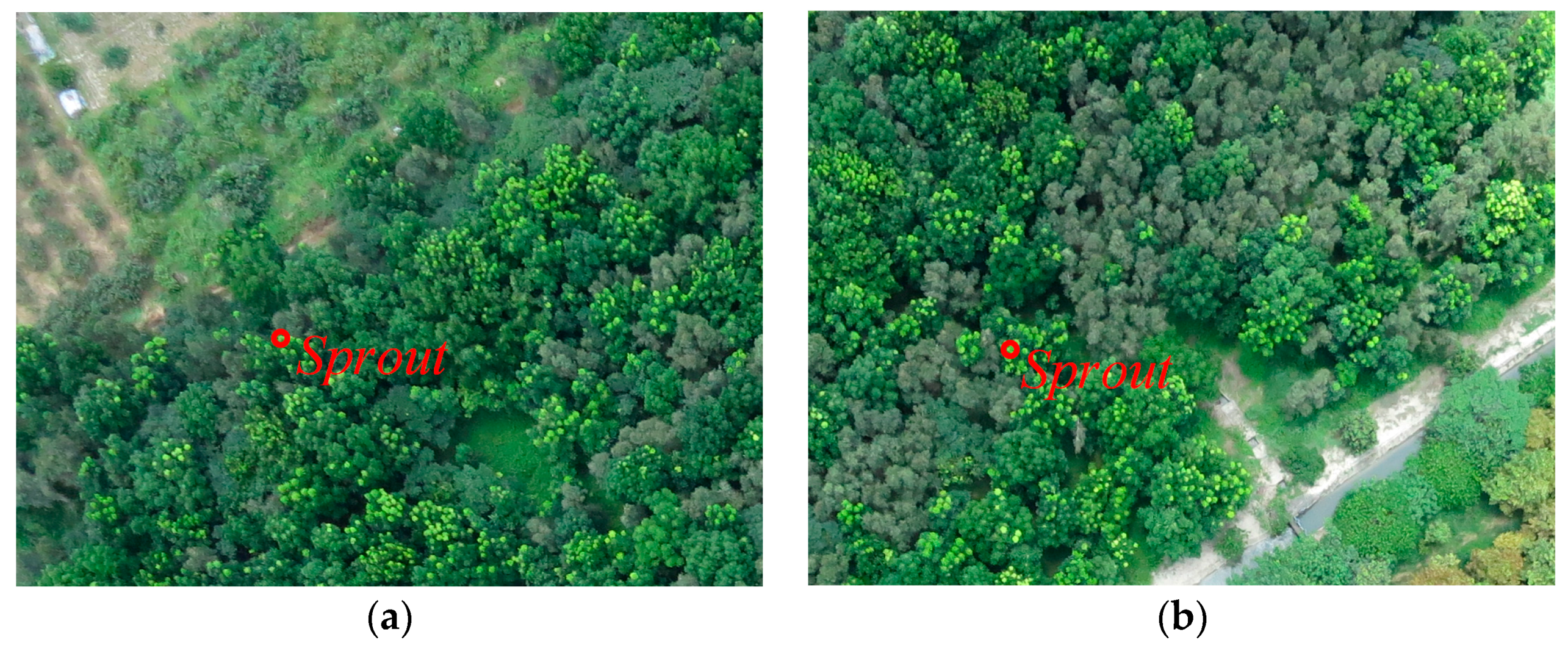
We applied the picture of a forest in the middle of Taiwan taken by a Canon PowerShot S110 camera on an eBee RTK drone flying at an altitude of 239.2 ft on 12 July 2014. This image has R, G, and B bands. Data acquisition took place under wonderful weather conditions. The ground pixel size is 6 cm, the original image resolution is 1000 × 1300 pixels, and the actual area of the full image is 60 m × 78 m. The data have been successfully used to derive forest canopy height model [50] and the desired target d for the target detection algorithm in this paper is the desired target that is selected randomly in the experimental image, as shown in Figure 10. The red circle is the target d for detection.
3.2.2. Ground Truth
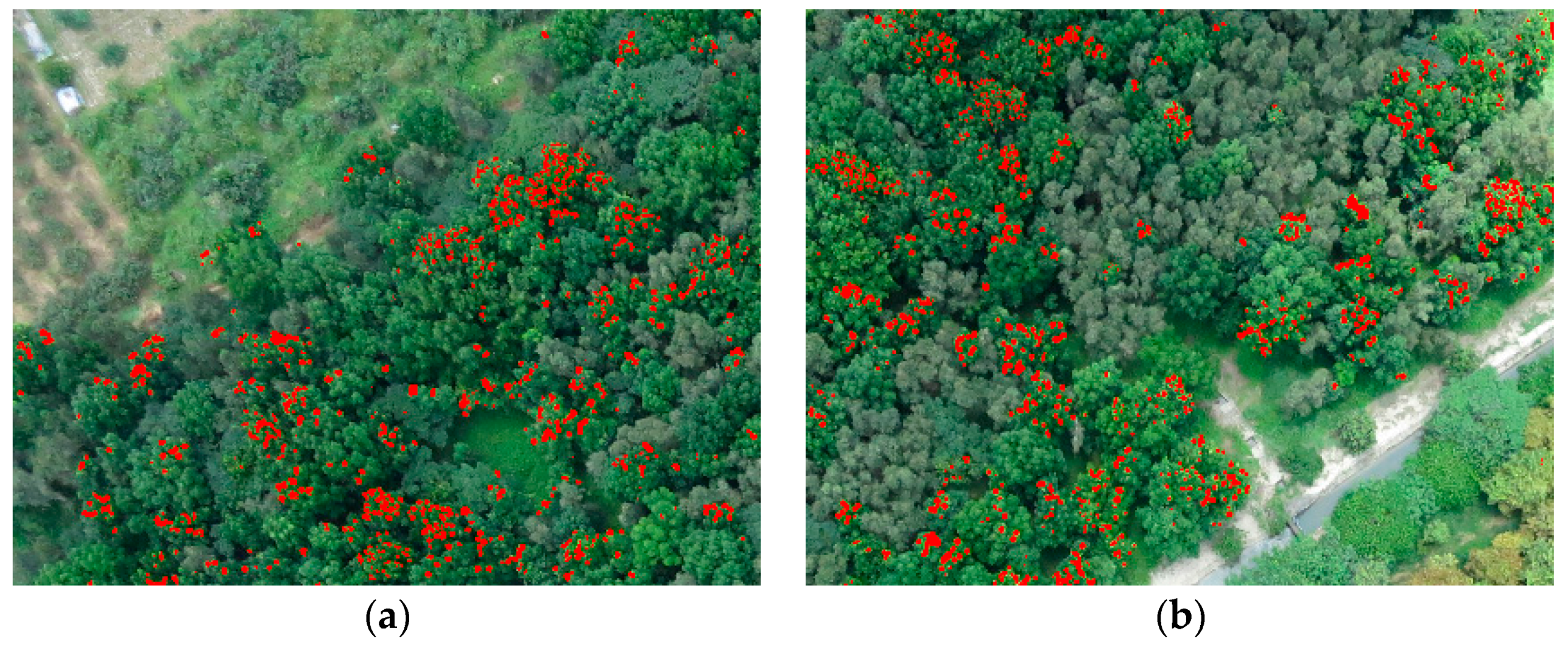
As shown in Figure 11, the NGLs can be visually interpreted due to their appearance of being bright and light green and is aggregated over tree crowns. According to a row of several years of inventory, the ground truth of the NGL over the images were visually interpreted and also validated in situ. In order to quantify and compare the effects of different target detection methods, there must be a NGL detection map as the standard and measure, i.e., ground truth of Region 1 and Region 2, as shown in Figure 12. Table 2 tabulates the number of pixels in NGL and non-NGL for Region 1 and 2. The NGL are only about 3–4% of the entire images.
3.3. Evaluation of Detection Results
The research methods used in this study were introduced in previous sections. In order to validate whether the three methods that are proposed herein can improve the original global CEM, two methods for evaluating the precision are used in this paper. The first method is the ROC curve [51,52,53], which is used to calculate the detection effect of a hyperspectral algorithm. The second method is Cohen’s kappa [54], which is an evaluation method extensively used in biology to calculate the model precision. In order to perform quantitative analysis, we further calculated the area under curve (AUC) for each ROC curves and overall accuracy (ACC).
3.3.1. ROC Curve
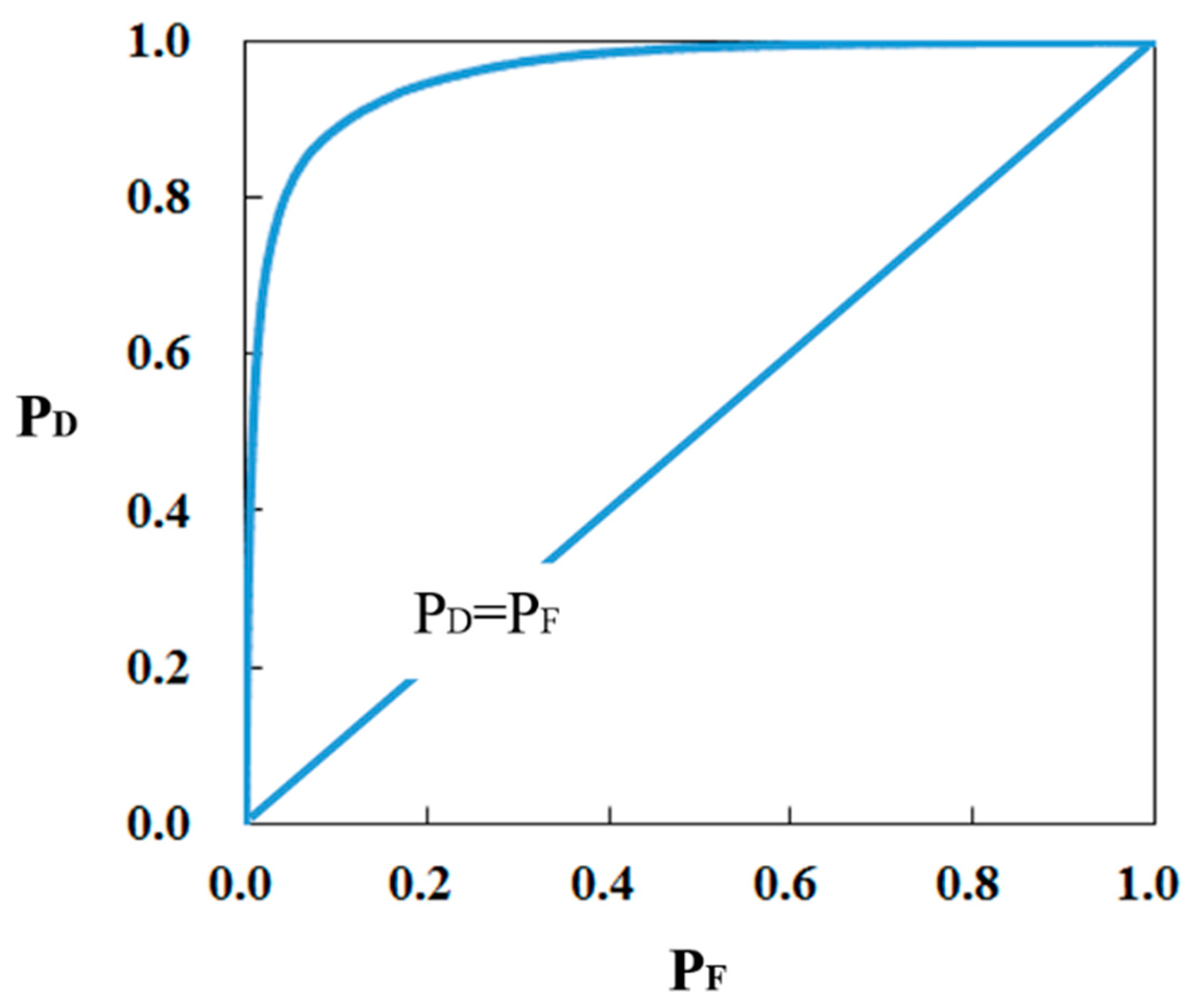
The main concept of ROC analysis [51,52,53] is a binary classification model, meaning there are only two classes of output, such as positive/negative, pass/failure, animal/non-animal, etc. For classification, a threshold must be given, and the threshold separates two classes. The probability of detection power (PD) and false alarm probability (PF) may differ under different thresholds. If the threshold is too high, then too many NGL will be estimated as non-NGL. If it is too low, then there will be more false alarms. To avoid this condition, PD and PF are calculated, respectively, by using different thresholds, and all threshold (τ) and PD and PF are drawn to obtain a ROC curve, as shown in Figure 13.
The optimum threshold (τ) depends on PD and PF to separate the NGL from the background, defined as:
As we hope that PD is larger the better and that PF is smaller the better, then the optimum threshold (τ) can be obtained on this condition. According to the detection result and practical situation, an Error Matrix can be given.
Generally, the weights of and in Equation (11) are 0.5; as their weights are identical, it is often ignored. The weight of Equation (11) can be adjusted depending on different applications.
3.3.2. Cohen’s Kappa
Cohen’s kappa coefficient is a statistical evaluation method for measuring the consistency between the two classes. In image processing, the effect of a detector is generally measured by the ROC Curve, whereas Cohen’s kappa is extensively used in biology to measure the efficiency of a detector. Cohen’s kappa is an algorithm using the result of binarization to evaluate and calculate consistency. It uses the error matrix identical with the ROC Curve to calculate the kappa value.
According to Table 3, Cohen’s kappa can be defined as
where represents the observation consistency (observed proportionate agreement) and represents the desired consistency (probability of random agreement). The K value ranges from −1 to 1. If the K value is smaller than 0, the detected result is worse than the stochastic prediction.
3.4. Experimental Results
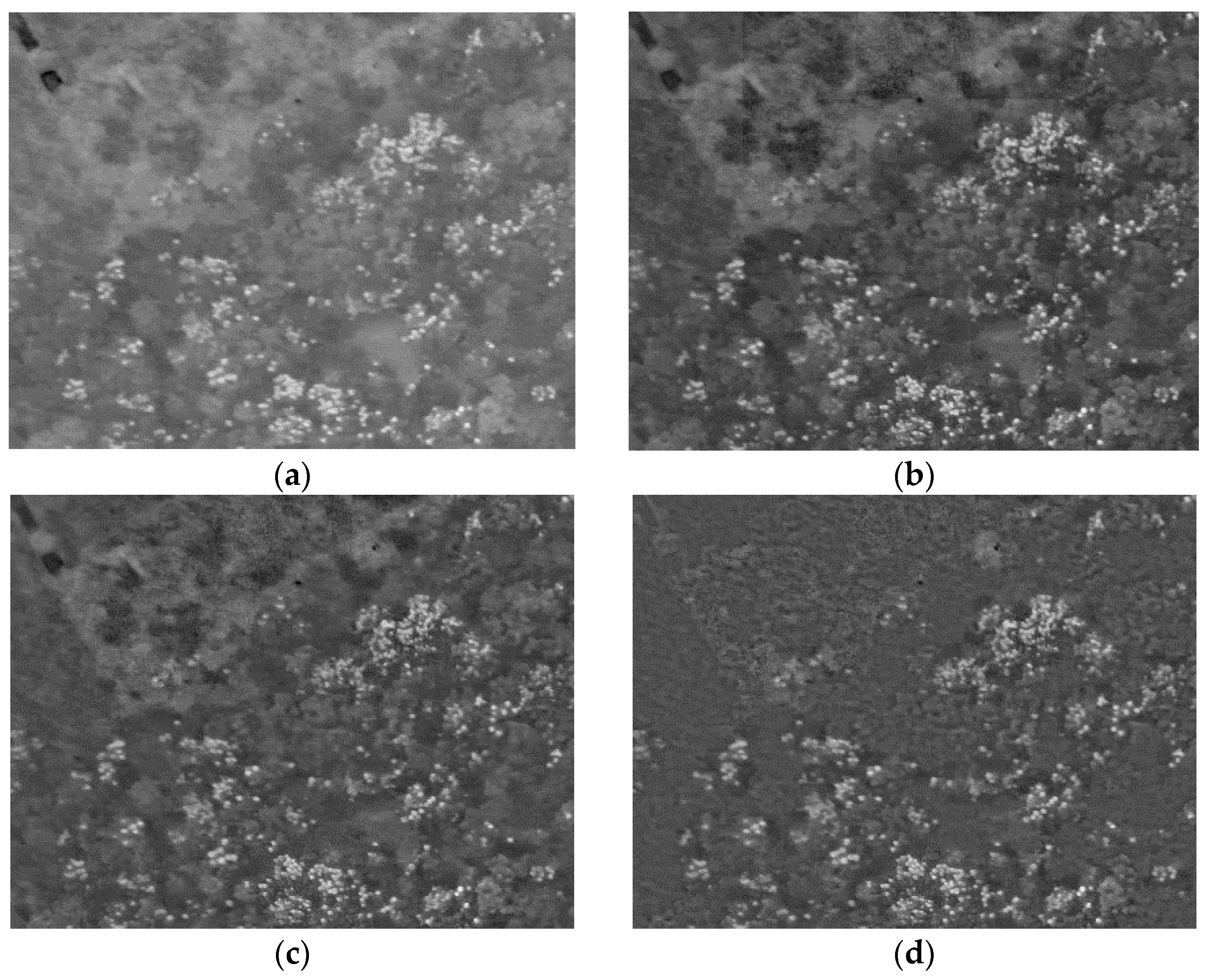
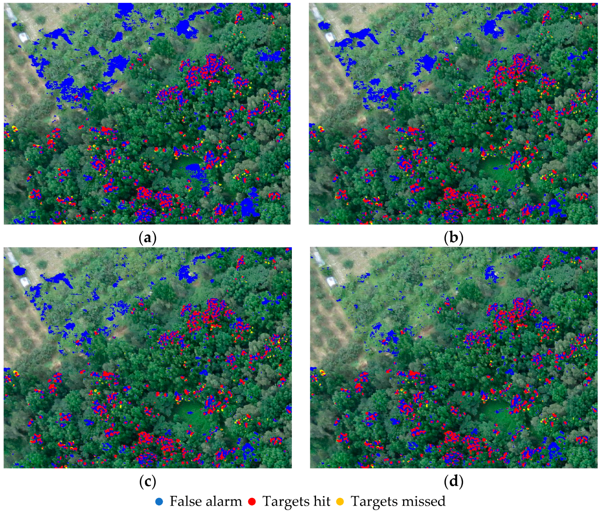
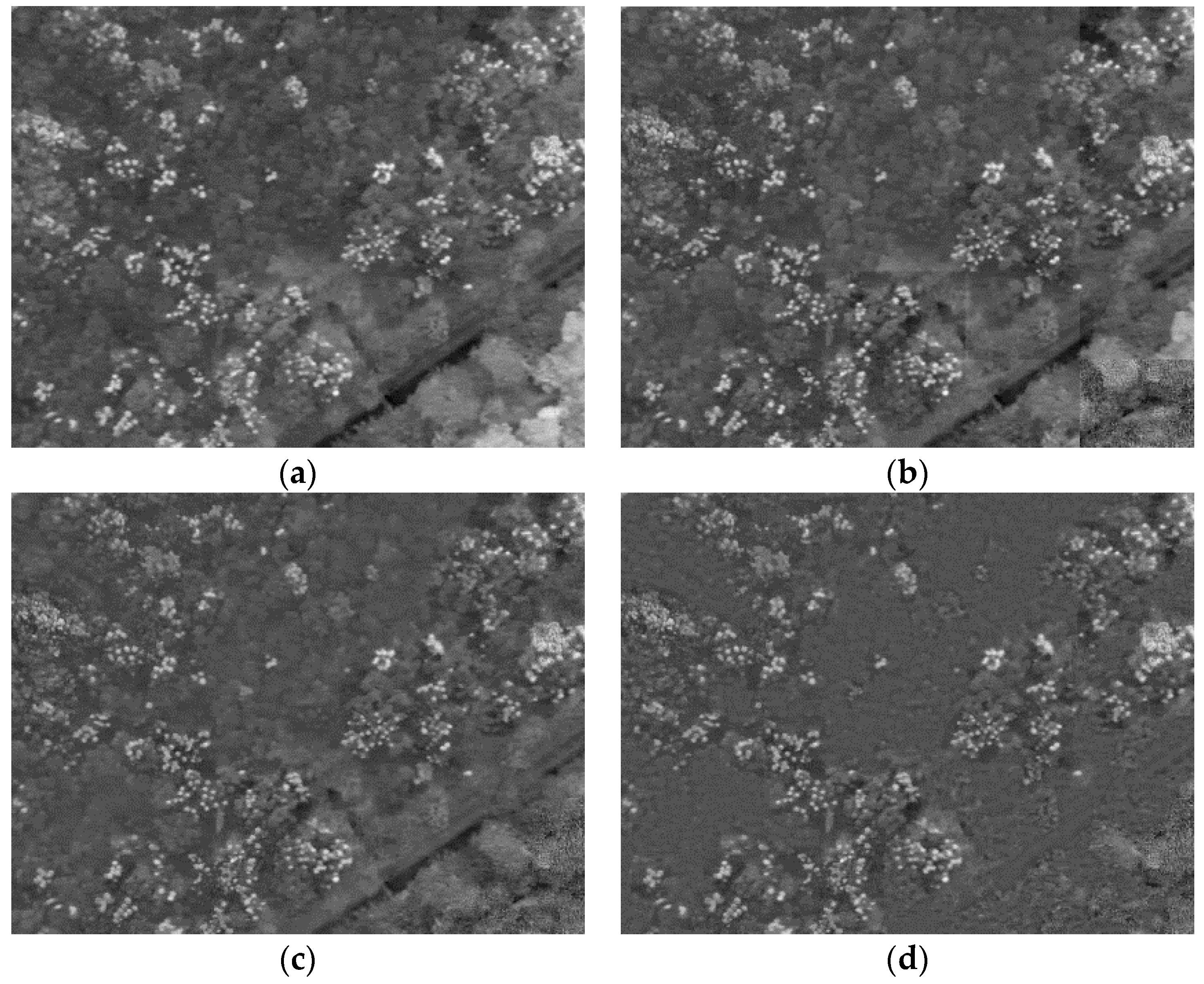
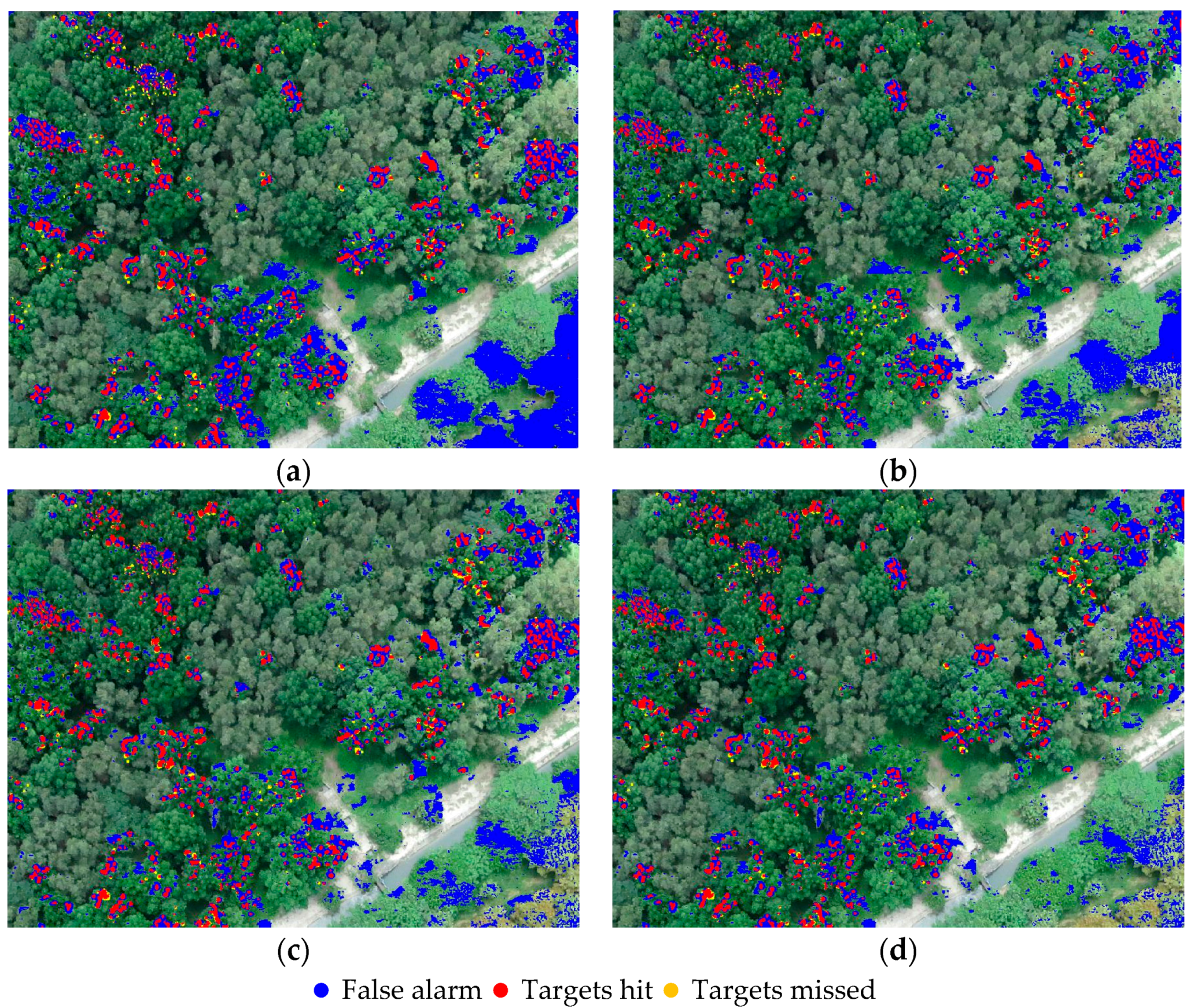
The brighter pixels in the detection maps of Figure 14 and Figure 15 represent the higher probability of NGL and highlight the pixels of targets hit in red points, the pixels of a false alarm in blue points, the pixels of targets missing in yellow points in Regions 1. By visually inspecting the Figures, the Subset CEM and SW CEM detectors seemed to perform slightly better than traditional CEM in terms of NGL pixel detection. Figure 16 and Figure 17 represent the higher probability of NGL and highlight the pixels of targets in Region 2. Obviously, the results of ASW CEM in Figure 15d and Figure 17d reduce plenty of false alarm pixels.
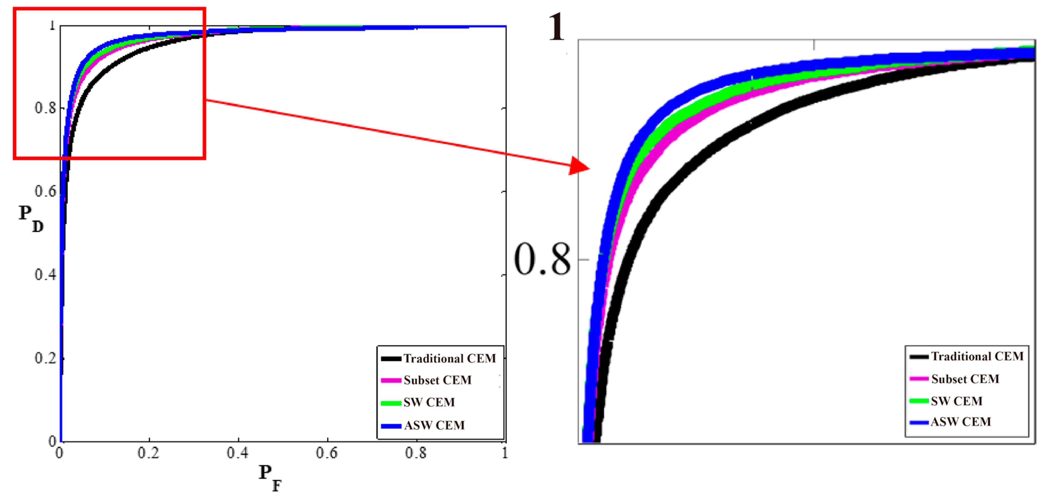
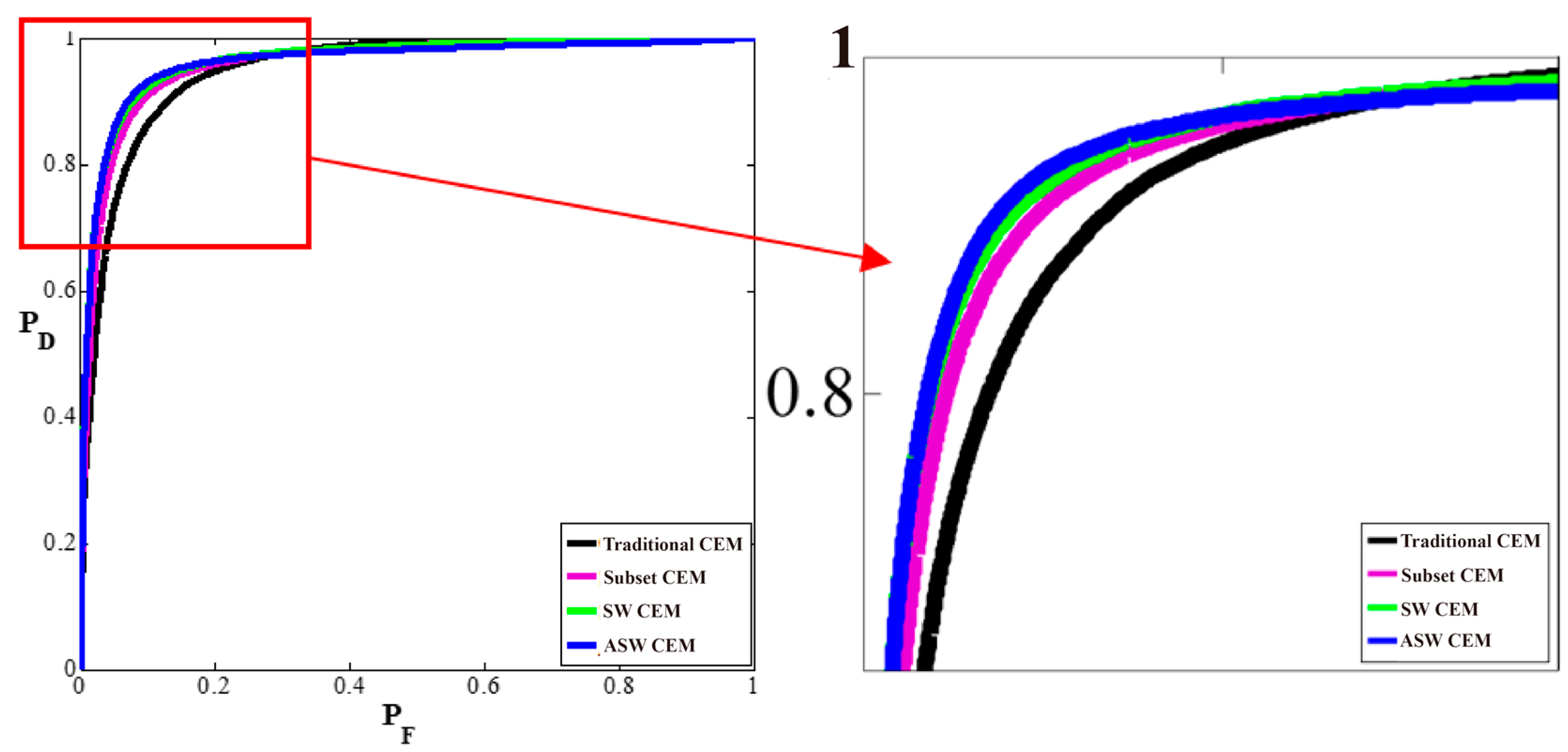
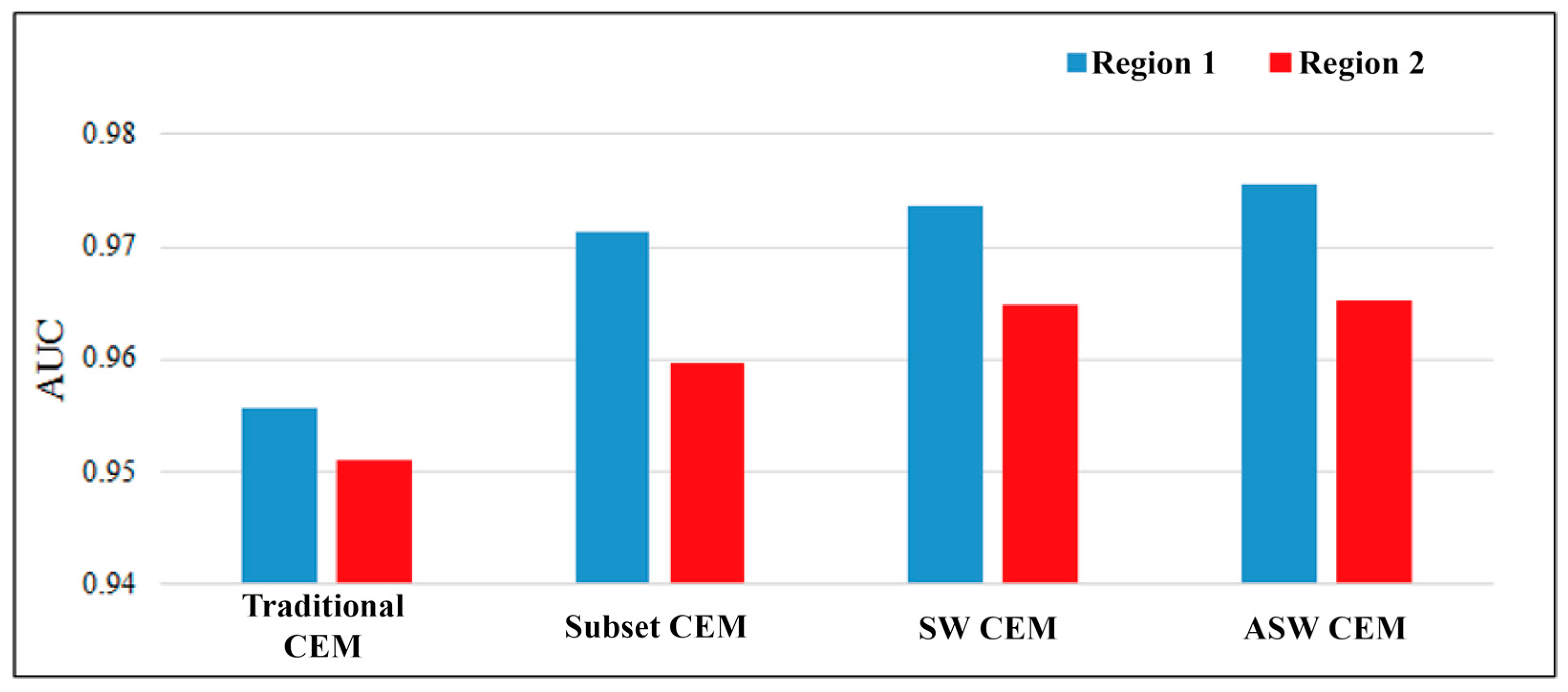
Figure 18 and Figure 19 show the ROC curves of traditional CEM and our proposed three window based CEMs. Table 4 and Table 5 show the AUC calculated, according to the ROC Curve in the experimental images of different regions and the evaluation of PD, PF, overall accuracy (ACC), and kappa under the optimum threshold.
The performance of each detection method can be judged according to its ROC curve. Different target detection algorithms have different AUCs (Area under the Curve of ROC). Generally speaking, the value of AUC is 0~1, and the performance of a detection method can be judged according to the AUC value. If AUC = 1, then the detector is almost perfect. When this detector is used, there are at least two thresholds, so the result appears to be ideal. If AUC is 0.5~1, then this detector is better than a random guess. If AUC is just equal to 0.5—as shown in Figure 13, when the detection power (PD) is equal to the false alarm probability (PF), meaning that the result is the same as a random guess, like flipping a coin—then the probability of front and back is 1/2. If AUC < 0.5, then the result is worse than a random guess, and the resulting target and the background may be inverted. Put briefly, the larger the AUC value is, the more correct is the detection method. According to Figure 16 and Figure 17, the three proposed CEMs have higher AUC than the traditional CEM.
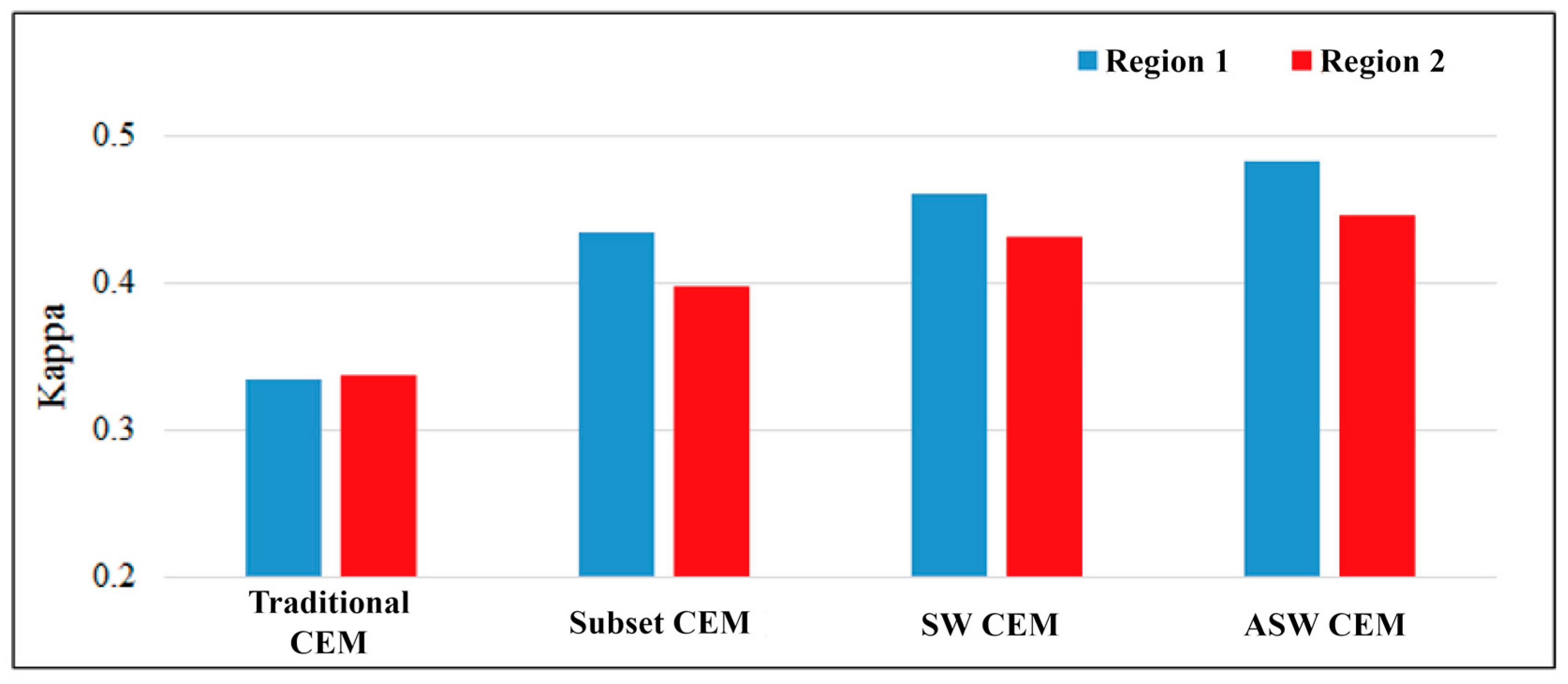
Finally, according to the data of ROC, kappa, and the error matrix in Table 4 and Table 5, in the three images of different resolutions of the two regions, respectively, ASW performs better than the other algorithms. The performance of TPR is slightly different from that of the other algorithms. However, in terms of the false alarm, ASW CEM can effectively reduce the detection of non NGL pixels, which thus can increase overall accuracy and the Kappa value of image detection. This result means that ASW CEM has a better detection result than the other algorithms. Figure 20 and Figure 21 illustrate the comparison of traditional CEM and our proposed three window based CEMs in the results of AUC and Kappa.
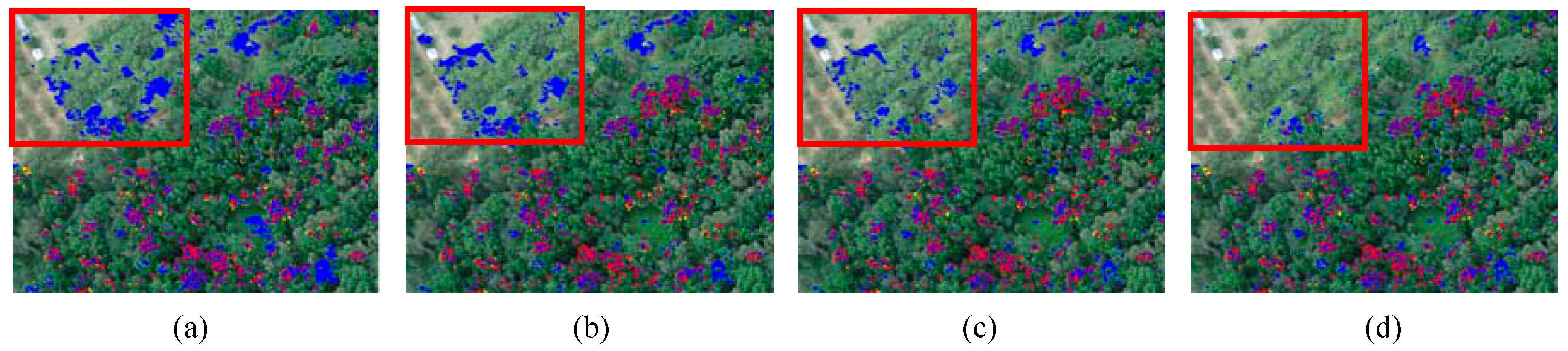
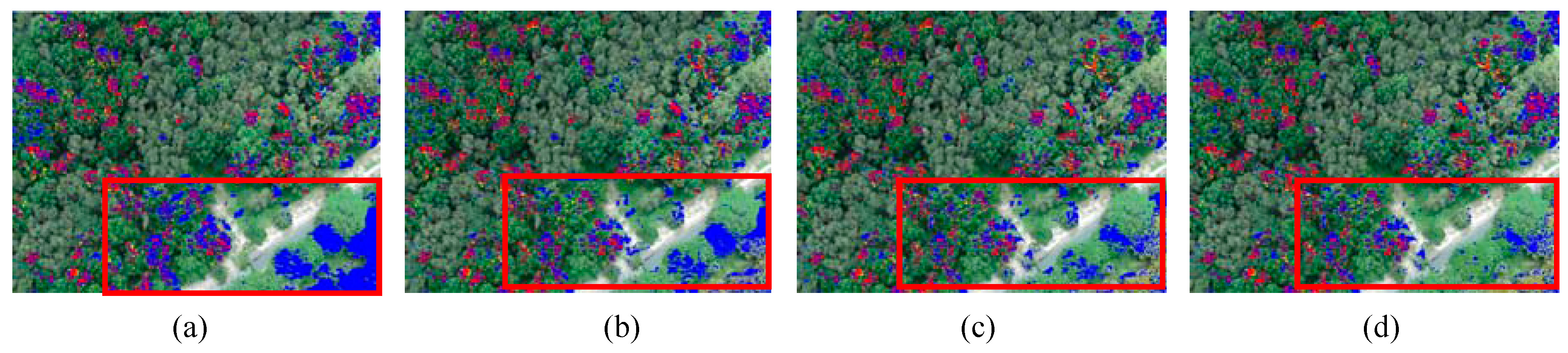
Figure 22 and Figure 23 highlight parts of two regions where a false alarm is likely to occur. In those regions where the false alarm is likely to occur in the two images, it is observed that the CEM algorithm is likely to misrecognize similar RGB values as NGL. Our proposed algorithms using local autocorrelation matrix S in Equation (10), such as Subset CEM, SW CEM, and ASW CEM, are likely to suppress the background of the region, so as to reduce the false alarm rate. Based on the experimental results, ASW CEM performs the best effect.
In order to the validate the influence of the window size for Subset CEM and SW CEM, Table 6 and Table 7 tabulate the detection results of various window sizes in Region 1. As seen, various window sizes of Subset CEM and SW CEM produce very similar results. On the other hand, the window size of Subset CEM and SW CEM are not sensitive to the final performance; thus, it is not the critical parameter for the detectors.
3.5. Computing Time
This section calculates the computing time in seconds by running CEM, Subset CEM, SW CEM, and ASW CEM on two real image scenes using MATLAB where the computer environment used for experiments was 64-bit Windows operating system with Intel i7-4710, CPU 2.5 Ghz, and 16 GB memory (RAM). In the two real image scenes, ASW CEM improves detection accuracy, the false alarm rate, and evaluation consistency better than the other algorithms, but the detection time of using local autocorrelation matrix S is longer than the traditional CEM, as shown in Table 8. It is noted that OSGP is not included in the computing time. The time listed in Table 8 is the execution time for each algorithm only. The time in ASW CEM also includes the time of acquiring the rate of NGL.
From computation perspective, calculating the inverse of the matrix takes most of time during computation. Since SW CEM needs to recalculate the inverse of S in Equation (10) in every pixel with the fixed window, in this case, it takes the longest time. AWS CEM can adjust the window size, and so the computing time is the second longest. In the best results of ASW CEM, the detection time is longer than CEM, but all of the evaluated data are enhanced significantly, meaning the ASW CEM algorithm consumes more detection time to increase accuracy, but the increment rate of result is higher. When compared to real time processing [16,55,56,57,58], the time is not a main consideration in this study. On the contrary, if the computing time is the issue, Subset CEM provides the reasonable improvement, with no computing time penalty. In this case, Subset CEM also can be applied in the some other applications.
Disregarding the minor defect of a long detection time, ASW CEM performs better in enhancement than the other algorithms, because ASW CEM can change the size of the sliding window according to the rate of the sprout around the current pixel.
4. Discussion
A variety of target detection techniques have been published during the last few decades [12,13,14,15,25,59], with several studies applying support vector machines (SVM) [60] or Fisher’s linear discriminant analysis (FLDA) [60] to solve target detection problems as a binary classification problem [61,62,63,64,65]. These algorithms require a number of classes, and their class distribution model must be known in advance. In order to avoid any biased selection of training samples, the partition must be performed randomly. In other words, training samples must be randomly selected from a dataset to form a training sample set for cross validation. As a result, such a validation is not repeatable and cannot be re-produced. The results are inconsistent. To alleviate this dilemma, this paper proposes a novel Constrained Energy Minimization (CEM) based technique that takes advantage of spectral and spatial information and developed Optimal Signature Generation Process (OSGP) in terms of the iterative process point of view to solve the issues mentioned above. CEM only requires one desired target information for the specific target of interest, regardless of other background information, which is its major advantage. Theoretically, CEM subpixel detection is generally performed by two operations that involve background suppression and matched filter [16]. First, it performs background suppression via the inverse of R so as to enhance a detected target contrast against the background. Second, CEM operates a matched filter using d as the desired matched signature so as to increase intensity of the target of interest. Since only one target signature can be used as the d in Equation (5), selecting an appropriate d is a very crucial step for detection results. Although CEM has many applications [27,30,31], very few studies investigated the issues of selecting a desire target signature. Therefore, this paper developed the Optimal Signature Generation Process (OSGP) to resolve this issue.
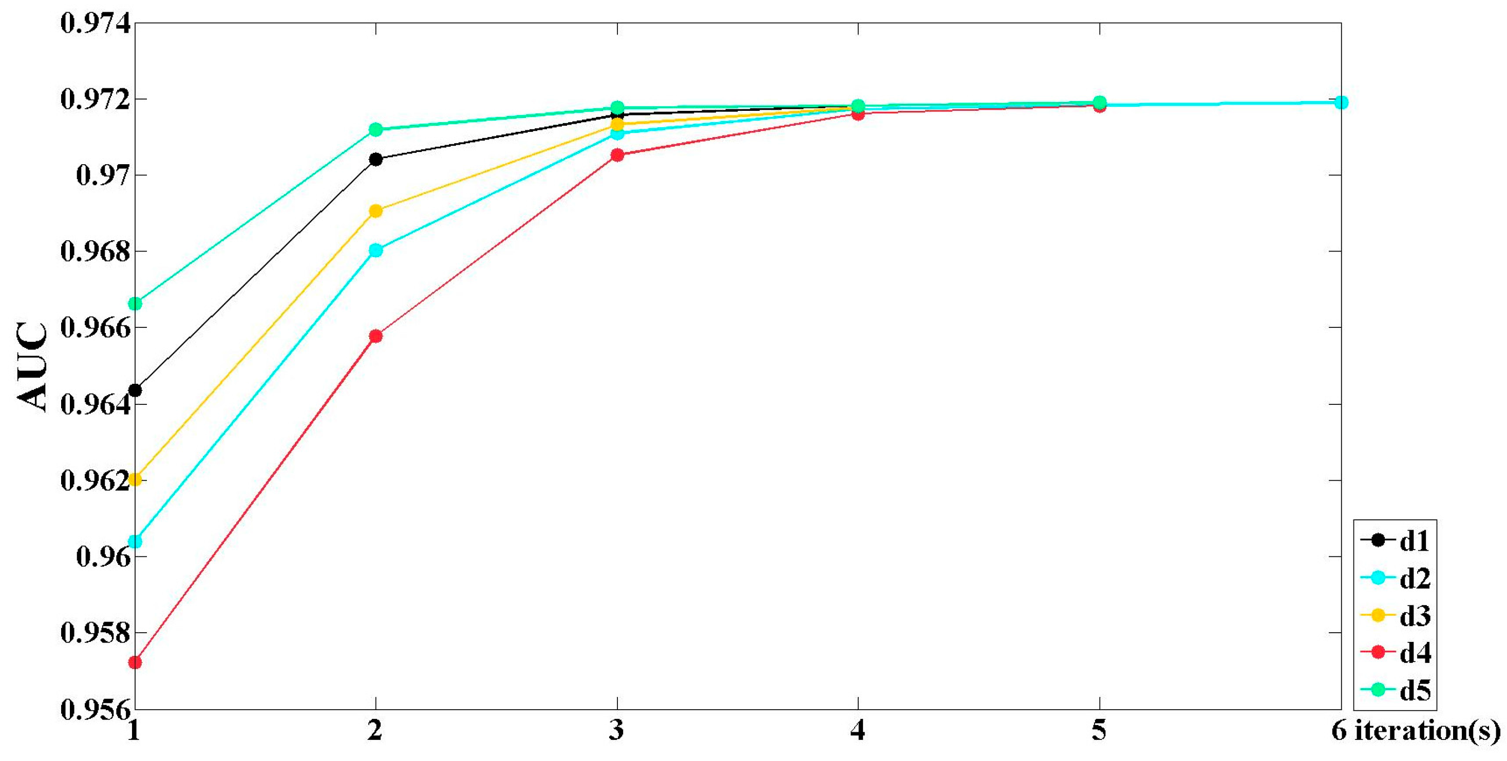
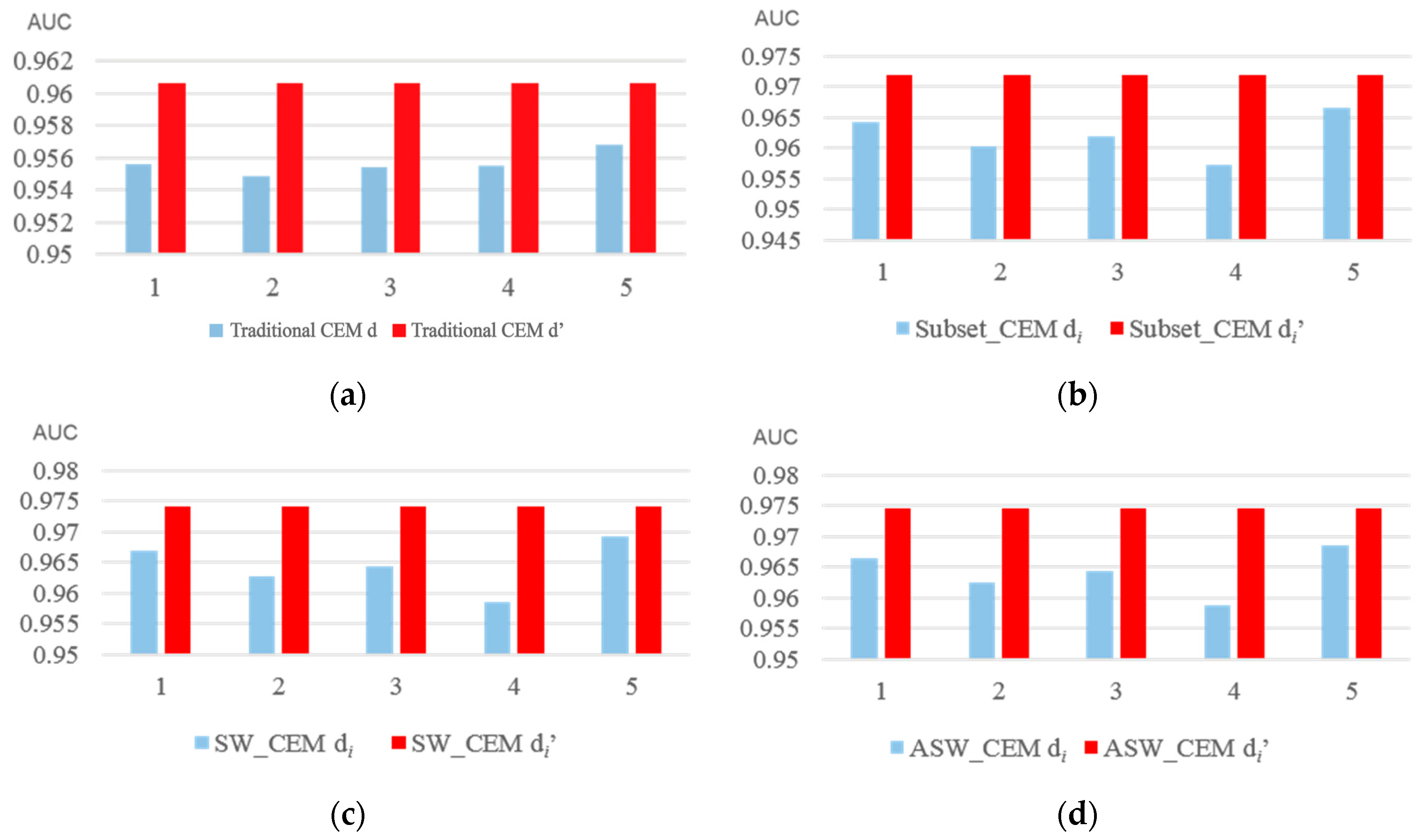
When compared to the classification based approaches that require very precise prior knowledge to generate a set of training samples and features, applying OSGP on the proposed CEM based methods required only one target signature information and provided stable results even if the initial desire target information is bias or not reliable. In the iterative process of OSGP in Figure 24, the iteration results of different desired signatures d after different numbers of iterations give a stable AUC result, so that the originally worse desired target obtains a relatively better desired target. Figure 25 shows different d’s have different results in the same algorithm. However, the d’ iterated by OSGP used in CEM, Subset CEM, SW CEM, and ASW CEM can enhance the original desired target to some extent. Moreover, the results are approximately identical, meaning OSGP can determine the appropriate desired target automatically when selecting inappropriate d as initial, and the result is still very stable.
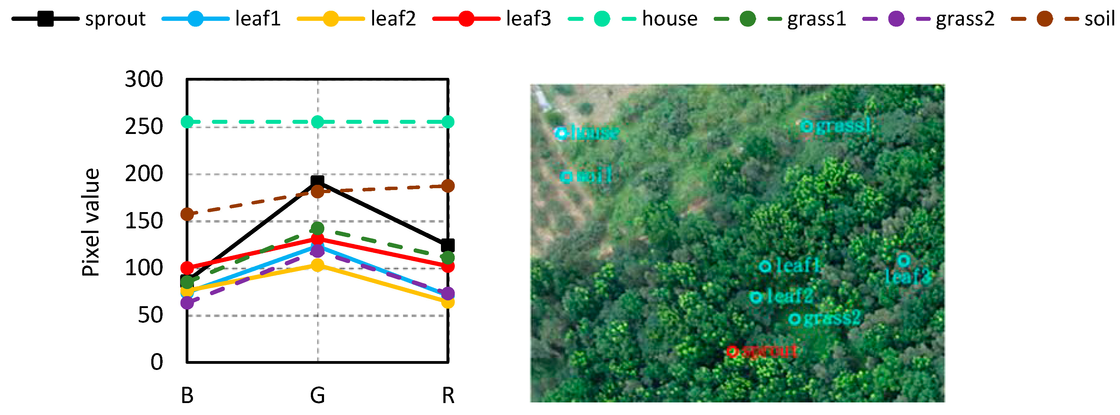
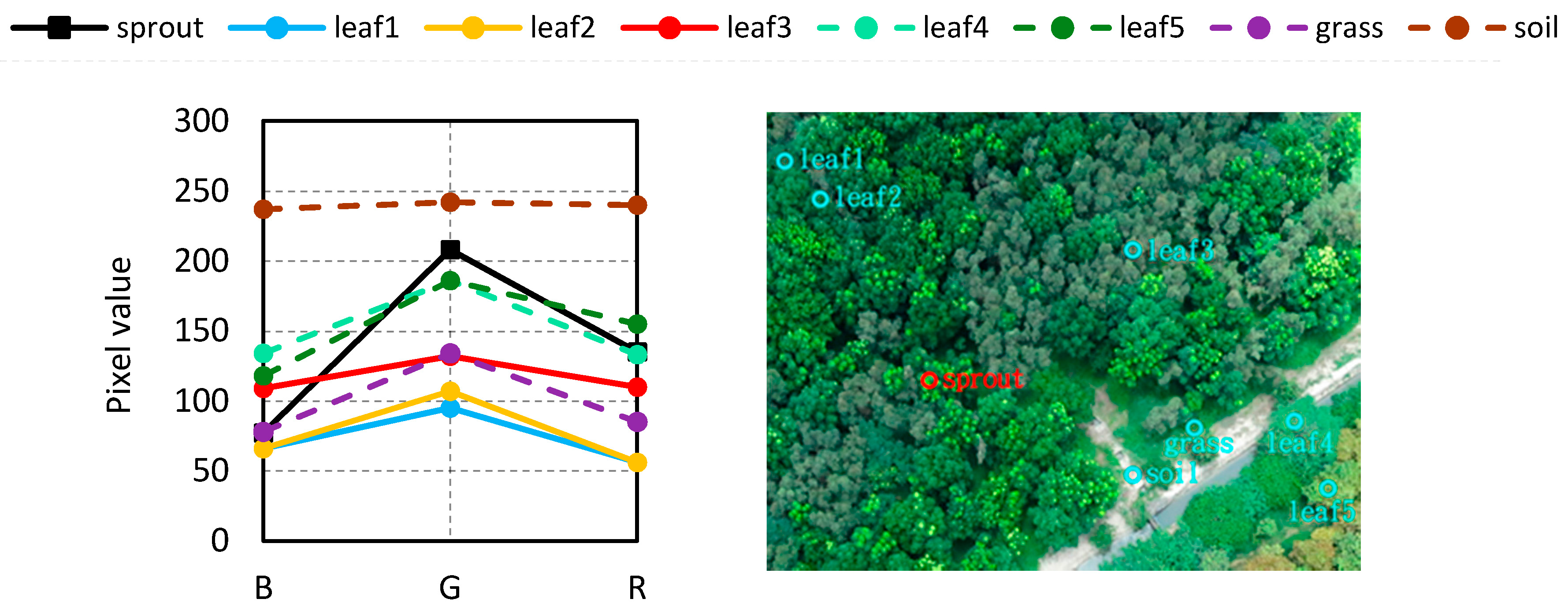
CEM technique only takes advantages of spectral information to detect target of interests. However, when spectral information is insufficient to distinguish between targets and some materials have similar spectral signature, this likely causes false alarms in the multispectral images. In this case, our proposed window-based techniques actually include spatial information into the CEM algorithms via fixed or adaptive windows to compensate for the insufficient spectral information. According to the experimental results and the resulting images in Figure 14, Figure 15, Figure 16 and Figure 17, among our proposed local CEM algorithms, the Subset CEM, Sliding Window-based CEM (SW CEM) of the fixed window size, or Adaptive Window-based CEM (ASW CEM) enhances the contrast between the target and the background better than the general CEM. Because the autocorrelation matrix R of the CEM algorithm is different, CEM uses R of the full image, whereas our proposed local CEMs uses local autocorrelation matrix S in Equation (10) to suppress the background. According to effect of the background suppression [58], it is obvious that using local autocorrelation S is better than global autocorrelation R in this study. Figure 26 and Figure 27 show the RGB signatures corresponding to different objects in the study site. As seen, some RGB signatures of leaves and grass are very close to NGL. In the upper left of Region 1, as the grass is too similar to the sprout shown in Figure 26, the CEM detection is likely to give a false alarm. Because the R that is used by CEM is generated according to the pixel value of the full image, the difference between NGL and grass is not obvious in the full image. In the entire image, the house and soil are larger than the RGB difference between grass and the sprout, and so the grass is likely to be misrecognized as NGL. On the contrary, in our proposed CEM based algorithms using S, because S is generated by pixels around the current pixel value and the proportion of soil and house is not high in a small area, the difference in RGB values between grass and NGL is enlarged, and the grass is likely to be suppressed, thus reducing the false alarm rate. In the same way, the lower right of Region 2 also easily gives a false alarm. Because the pixel values of some leaves are very similar to NGL in the region shown in Figure 27, when R is used to suppress the background, it is likely to be influenced by pixel values with a larger difference, and this problem can be solved by using S.
ASW CEM can change the size of the sliding window, according to the ratio of NGL around the current pixel. When there are too many NGL in the window, the difference between them is likely to be enlarged, and NGL that is very different from the desired target will be suppressed, leading to detection omission. Therefore, the sliding window shall be enlarged to reduce the rate of NGL and enhance the difference from the background, thus increasing the detected value. On the contrary, if the rate of NGL is too low, then the difference between backgrounds increase, and the RGB values that are similar to NGL is likely to be misrecognized. At this point, the sliding window is shrunk, the rate of NGL increases, the difference between NGL and background are more apparent, and the result value of the non-NGL is reduced for suppression. When NGL are enhanced and background is suppressed; their difference is enlarged, so as to highlight NGL.
Briefly, CEM technique was originally designed to catch (1) low probability of infrequent occurrence, (2) relatively small sample size, and (3) most importantly, the target pixel has spectrally distinct from its surrounding pixels [16]. Obviously, the NGL in RGB images shows the same features. This explains why the window-based CEM techniques can achieve satisfied results of NGL detection even only three spectral signatures is used.
5. Conclusions
Constant leaf sprouting and development can be an indication of healthy trees in beneficial environmental circumstances. This paper investigated the feasibility of NGL detection using hyperspectral detection algorithms in UAV bitmap images. Since the bitmap images only provide RGB values, using a traditional subpixel detector CEM presents false alarm issue. In order to address this issue, three window based CEMs are proposed in this paper. First, Subset CEM is developed to split the image into different small images, according to different regions. Second, the sliding window-base CEM was proposed to extract the RGB values around the current pixel to calculate autocorrelation matrix S. Third, this paper further proposed adaptive window-based CEM (ASW CEM), which can change the window size automatically according to NGL around the current pixel. ASW CEM extracts and calculates autocorrelation matrix S, increasing the contrast between NGL and the background, so as to highlight NGLs and to suppress the background. Last but not the least, in order to reduce the effect of the quality of the desired target selected for CEM, this paper designed OSGP to generate a stable desired target during iterations. The experimental results show that our proposed approaches can effectively reduce the errors resulting from a false alarm so as to obtain more appropriate desired target and stable results for newly grown tree leaves in UAV images.
Acknowledgments
The authors would like to acknowledge the support provided by projects MOST 106-2221-E-224-055 and MOST 105-2119-M-415-002 funded by the Ministry of Science and Technology, Taiwan, ROC.
Author Contributions
S.-Y.C. conceived and designed the algorithms and wrote the paper; C.L. analyzed the data, contributed data collection, reviewed the paper and organized the revision. C.-H.T. and S.-J.C. performed the experiments.
Conflicts of Interest
The authors declare no conflict of interest.
References
- Forest Resources Assessment (FAO). Global Forest Resources Assessment 2015—How Are the World’s Forests Changing; Food and Agricultural Organization of United Nations: Rome, Italy, 2015. [Google Scholar]
- Lin, C.; Dugarsuren, N. Deriving the Spatiotemporal NPP Pattern in Terrestrial Ecosystems of Mongolia using MODIS Imagery. Photogram. Eng. Remote Sens. 2015, 81, 587–598. [Google Scholar] [CrossRef]
- Lin, C.; Thomson, G.; Popescu, S.C. An IPCC-Compliant Technique for Forest Carbon Stock Assessment Using Airborne LiDAR-Derived Tree Metrics and Competition Index. Remote Sens. 2016, 8, 528. [Google Scholar] [CrossRef]
- Lin, C.; Chen, S.-Y.; Chen, C.-C.; Tai, C.-H. Detecting Newly Grown Tree Leaves from Unmanned-Aerial-Vehicle Images using Hyperspectral Target Detection Techniques. ISPRS J. Photogramm. Remote Sens. 2017. in review. [Google Scholar]
- Lin, C.; Wu, C.C.; Tsogt, K.; Ouyang, Y.C.; Chang, C.I. Effects of Atmospheric Correction and Pansharpening on LULC Classification Accuracy using WorldView-2 Imagery. Inf. Process. Agric. 2015, 2, 25–36. [Google Scholar] [CrossRef]
- Götze, C.; Gerstmann, H.; Gläßer, C.; Jung, A. An approach for the classification of pioneer vegetation based on species-specific phenological patterns using laboratory spectrometric measurements. Phys. Geogr. 2017, 38, 524–540. [Google Scholar] [CrossRef]
- Burai, P.; Deák, B.; Valkó, O.; Tomor, T. Classification of Herbaceous Vegetation Using Airborne Hyperspectral Imagery. Remote Sens. 2015, 7, 2046–2066. [Google Scholar] [CrossRef]
- Mohan, M.; Silva, C.A.; Klauberg, C.; Jat, P.; Catts, G.; Cardil, A.; Hudak, A.T.; Dia, M. Individual Tree Detection from Unmanned Aerial Vehicle (UAV) Derived Canopy Height Model in an Open Canopy Mixed Conifer Forest. Forest 2017, 8, 340. [Google Scholar] [CrossRef]
- Wallace, L.; Lucieer, A.; Watson, C.S. Evaluating Tree Detection and Segmentation Routines on Very High Resolution UAV LiDAR Data. IEEE Trans. Geosci. Remote Sens. 2014, 52, 7619–7628. [Google Scholar] [CrossRef]
- Dugarsuren, N.; Lin, C. Temporal variations in phenological events of forests, grasslands and desert steppe ecosystems in Mongolia: A Remote Sensing Approach. Ann. For. Res. 2016, 59, 175–190. [Google Scholar]
- Popescu, S.C.; Zhao, K.; Neuenschwander, A.; Lin, C. Satellite lidar vs. small footprint airborne lidar: Comparing the accuracy of aboveground biomass estimates and forest structure metrics at footprint level. Remote Sens. Environ. 2011, 115, 2786–2797. [Google Scholar] [CrossRef]
- Zeng, M.; Li, J.; Peng, Z. The design of Top-Hat morphological filter and application to infrared target detection. Infrared Phys. Technol. 2006, 48, 67–76. [Google Scholar] [CrossRef]
- Gao, C.; Meng, D.; Yang, Y.; Wang, Y.; Zhou, X.; Hauptmann, A.G. Infrared patch-image model for small target detection in a single image. IEEE Trans. Image Process. 2013, 22, 4996–5009. [Google Scholar] [CrossRef] [PubMed]
- Debes, C.; Zoubir, A.M.; Amin, M.G. Enhanced detection using target polarization signatures in through-the-wall radar imaging. IEEE Trans. Geosci. Remote Sens. 2012, 50, 1968–1979. [Google Scholar] [CrossRef]
- Qi, S.; Ma, J.; Tao, C.; Yang, C.; Tian, J. A robust directional saliency-based method for infrared small-target detection under various complex backgrounds. IEEE Trans. Geosci. Remote Sens. Lett. 2013, 10, 495–499. [Google Scholar]
- Chang, C.I. Real-Time Progressive Hyperspectral Image Processing: Endmember Finding and Anomaly Detection; Springer: Berlin, Germany, 2016. [Google Scholar]
- Chang, C.-I. Hyperspectral Data Processing: Algorithm Design and Analysis; Wiley: Hoboken, NJ, USA, 2013. [Google Scholar]
- Chang, C.-I. Hyperspectral Imaging: Techniques for Spectral detection and Classification; Kluwer Academic/Plenum Publishers: Dordrecht, The Netherlands, 2003. [Google Scholar]
- Harsanyi, J.C. Detection and Classification of Subpixel Spectral Signatures in Hyperspectral Image Sequences. Ph.D. Thesis, Department of Electrical Engineering, University of Maryland, Baltimore, MA, USA, 1993. [Google Scholar]
- Rees, G.; Rees, W.G. Physical Principles of Remote Sensing; Cambridge University Press: Cambridge, UK, 2013. [Google Scholar]
- Mahalanobis, P.C. On the generalized distance in statistics. Proc. Natl. Inst. Sci. India 1936, 2, 49–55. [Google Scholar]
- Kraut, S.; Scharf, L.L.; Butler, R.W. The adaptive coherence estimator: A uniformly most-powerful-invariant adaptive detection statistic. IEEE Trans. Signal Process. 2005, 53, 427–438. [Google Scholar] [CrossRef]
- Ren, H.; Chang, C.-I. Target-constrained interference-minimized approach to subpixel target detection for hyperspectral images. Opt. Eng. 2000, 39, 3138–3145. [Google Scholar] [CrossRef]
- Xue, B.; Yu, C.; Wang, Y.; Song, M.; Li, S.; Wang, L.; Chen, H.; Chang, C.I. A Subpixel Target Detection Approach to Hyperspectral Image Classification: Iterative Constrained Energy Minimization. IEEE Trans. Geosci. Remote Sens. 2017, 55, 5093–5114. [Google Scholar] [CrossRef]
- Sun, H.; Sun, X.; Wang, H.; Li, Y.; Li, X. Automatic target detection in high-resolution remote sensing images using spatial sparse coding bag-of-words model. IEEE Trans. Geosci. Remote Sens. 2012, 9, 109–113. [Google Scholar] [CrossRef]
- Chang, C.I.; Wang, Y.; Chen, S.Y. Anomaly Detection Using Causal Sliding Windows. IEEE J. Sel. Top. Appl. Earth Obs. Remote Sens. 2015, 8, 3260–3270. [Google Scholar] [CrossRef]
- Chang, C.I.; Schultz, R.C.; Hobbs, M.C.; Chen, S.Y.; Wang, Y.; Liu, C. Progressive Band Processing of Constrained Energy Minimization for Subpixel Detection. IEEE Trans. Geosci. Remote Sens. 2015, 53, 1626–1637. [Google Scholar] [CrossRef]
- Manolakis, D.; Marden, D.; Shaw, G.A. Hyperspectral image processing for automatic target detection applications. Linc. Lab. J. 2003, 14, 79–116. [Google Scholar]
- Nasrabadi, N.M. Hyperspectral target detection: An overview of current and future challenges. IEEE Signal Process. Mag. 2014, 31, 34–44. [Google Scholar] [CrossRef]
- Zou, Z.; Shi, Z. Hierarchical Suppression Method for Hyperspectral Target Detection. IEEE Trans. Geosci. Remote Sens. 2016, 54, 330–342. [Google Scholar] [CrossRef]
- Sun, K.; Geng, X.; Ji, L. A New Sparsity-Based Band Selection Method for Target Detection of Hyperspectral Image. IEEE Trans. Geosci. Remote Sens. Lett. 2015, 12, 329–333. [Google Scholar]
- Frost, O.L., III. An algorithm for linearly constrained adaptive array processing. Proc. IEEE. 1972, 60, 926–935. [Google Scholar] [CrossRef]
- Weinberg, G.V. An invariant sliding window detection process. IEEE Signal Process. Lett. 2017, 24, 1093–1097. [Google Scholar] [CrossRef]
- Castella, F.R. Sliding window detection probability. IEEE Trans. Aerosp. Electron. Syst. 1976, 6, 815–819. [Google Scholar] [CrossRef]
- Zhang, L.; Lin, J.; Karim, R. Sliding window-based fault detection from high-dimensional data streams. IEEE Trans. Syst. Man Cybern. Syst. 2017, 47, 289–303. [Google Scholar] [CrossRef]
- Noh, S.; Shim, D.; Jeon, M. Adaptive Sliding-Window Strategy for Vehicle Detection in Highway Environments. IEEE Trans. Intell. Transp. Syst. 2016, 17, 323–335. [Google Scholar] [CrossRef]
- Gao, G.; Liu, L.; Zhao, L.; Shi, G.; Kuang, G. An Adaptive and Fast CFAR Algorithm Based on Automatic Censoring for Target Detection in High-Resolution SAR Images. IEEE Trans. Geosci. Remote Sens. 2009, 47, 1685–1697. [Google Scholar] [CrossRef]
- Akkoul, S.; Ledee, R.; Leconge, R.; Harba, R. A New Adaptive Switching Median Filter. IEEE Signal Process. Lett. 2010, 17, 587–590. [Google Scholar] [CrossRef]
- Matteoli, S.; Diani, M.; Corsini, G. Impact of signal contamination on the adaptive detection performance of local hyperspectral anomalies. IEEE Trans. Geosci. Remote Sens. 2014, 52, 1948–1968. [Google Scholar] [CrossRef]
- Matteoli, S.; Veracini, T.; Diani, M.; Corsini, G. A locally adaptive background density estimator: An evolution for RX-based anomaly detectors. IEEE Geosci. Remote Sens. Lett. 2014, 11, 323–327. [Google Scholar] [CrossRef]
- Chang, C.-I. An information theoretic-based approach to spectral variability, similarity and discriminability for hyperspectral image analysis. IEEE Trans. Inf. Theory 2000, 46, 1927–1932. [Google Scholar] [CrossRef]
- Otsu, N. A threshold selection method from gray-level histograms. IEEE Trans. Syst. Man Cybern. 1979, 9, 62–66. [Google Scholar] [CrossRef]
- Hall, D.; Ball, G. Isodata: A Novel Method of Data Analysis and Pattern Classification; Stanford Research Institude: Menlo Park, CA, USA, 1965. [Google Scholar]
- MacQueen, J. Some methods for classification and analysis of multivariate observations. In Proceedings of the 5th Berkeley Symposium on Mathematical Statistics and Probability, Berkeley, CA, USA, 21 June–18 July 1965 and 27 December 1965–7 January 1966; University of California Press: Berkeley, CA, USA, 1967; pp. 281–296. [Google Scholar]
- Chen, H.M.; Lin, C.; Chen, S.Y.; Wen, C.H.; Chen, C.C.C.; Ouyang, Y.C.; Chang, C.I. PPI SVM-Iterative FLDA Approach to Unsupervised Multispectral Image Classification. IEEE J. Sel. Top. Appl. Earth Obs. Remote Sens. 2013, 6, 1834–1842. [Google Scholar] [CrossRef]
- Zhuang, H.; Deng, K.; Fan, H.; Yu, M. Strategies combining spectral angle mapper and change vector analysis to unsupervised change detection in multispectral images. IEEE Trans. Geosci. Remote Sens. 2016, 13, 681–685. [Google Scholar] [CrossRef]
- Lin, C.; Lin, C.H. Comparison of Carbon Sequestration Potential in Agricultural and Afforestation Farming Systems. Sci. Agric. 2013, 70, 93–101. [Google Scholar] [CrossRef]
- Lin, C.; Wang, J.J. The effect of trees spacing on the growth of trees in afforested broadleaf stands on cultivated farmland. Q. J. Chin. For. 2013, 46, 311–326. [Google Scholar]
- Lin, C.; Tsogt, K.; Zandraabal, T. A decompositional stand structure analysis for exploring stand dynamics of multiple attributes of a mixed-species forest. For. Ecol. Manag. 2016, 378, 111–121. [Google Scholar] [CrossRef]
- Lin, C.; Lo, K.L.; Huang, P.L. A classification method of unmanned-aerial-systems-derived point cloud for generating a canopy height model of farm forest. In Proceedings of the 2016 IEEE International Geoscience and Remote Sensing Symposium (IGARSS), Beijing, China, 10–15 July 2016; pp. 740–743. [Google Scholar]
- Burnett, R.; Brunstrom, A.; Nilsson, A.G. Perspectives on Multimedia: Communication, Media and Information Technology; John Wiley & Sons: Hoboken, NJ, USA, 2005. [Google Scholar]
- Chang, C.-I. Multiple-parameter receiver operating characteristic analysis for signal detection and classification. IEEE Sens. J. 2010, 10, 423–442. [Google Scholar] [CrossRef]
- Swets, J.A.; Pickett, R.M. Evaluation of Diagnostic Systems: Methods from Signal Detection Theory; Academic Press: Cambridge, MA, USA, 1982. [Google Scholar]
- Pontius, R.; Millones, M. Death to Kappa: Birth of quantity disagreement and allocation disagreement for accuracy assessment. Int. J. Remote Sens. 2011, 32, 4407–4429. [Google Scholar] [CrossRef]
- Chang, C.-I.; Ren, H.; Chiang, S.S. Real-time processing algorithms for target detection and classification in hyperspectral imagery. IEEE Trans. Geosci. Remote Sens. 2001, 39, 760–768. [Google Scholar] [CrossRef]
- Stellman, C.M.; Hazel, G.G.; Bucholtz, F.; Michalowicz, J.V.; Stocker, A.D.; Schaaf, W. Real-time hyperspectral detection and cuing. Opt. Eng. 2000, 39, 1928–1935. [Google Scholar] [CrossRef]
- Du, Q.; Ren, H. Real-time constrained linear discriminant analysis to target detection and classification in hyperspectral imagery. Pattern Recognit. 2003, 36, 1–12. [Google Scholar] [CrossRef]
- Chang, C.I. Real-Time Recursive Hyperspectral Sample and Band Processing: Algorithm Architecture and Implementation; Springer: Berlin, Germany, 2017. [Google Scholar]
- Zhang, L.; Zhang, L.; Tao, D.; Huang, X. Sparse transfer manifold embedding for hyperspectral target detection. IEEE Trans. Geosci. Remote Sens. 2014, 52, 1030–1043. [Google Scholar] [CrossRef]
- Vapnik, V.N. Statistical Learning Theory; Wiley: New York, NY, USA, 1998. [Google Scholar]
- Wu, Y.; Yang, X.; Plaza, A.; Qiao, F.; Gao, L.; Zhang, B.; Cui, Y. Approximate Computing of Remotely Sensed Data: SVM Hyperspectral Image Classification as a Case Study. IEEE J. Sel. Top. Appl. Earth Obs. Remote Sens. 2016, 9, 5806–5818. [Google Scholar] [CrossRef]
- Bo, C.; Lu, H.; Wang, D. Hyperspectral Image Classification via JCR and SVM Models with Decision Fusion. IEEE Trans. Geosci. Remote Sens. Lett. 2016, 13, 177–181. [Google Scholar]
- Xue, Z.; Du, P.; Su, H. Harmonic Analysis for Hyperspectral Image Classification Integrated With PSO Optimized SVM. IEEE J. Sel. Top. Appl. Earth Obs. Remote Sens. 2014, 7, 2131–2146. [Google Scholar] [CrossRef]
- Kang, X.; Xiang, X.; Li, S.; Benediktsson, J.A. PCA-Based Edge-Preserving Features for Hyperspectral Image Classification. IEEE Trans. Geosci. Remote Sens. 2017, 55, 7140–7151. [Google Scholar] [CrossRef]
- Roli, F.; Fumera, G. Support vector machines for remote-sensing image classification. Proc. SPIE 2001, 4170, 160–166. [Google Scholar]
Figure 1.
Schematic diagram for the autocorrelation matrix of the original image and subset images.

Figure 2.
Schematic diagram of the division of subset images by Subset CEM.

Figure 3.
Sliding window matrices of r(m,n) and r(m+1,n).

Figure 4.
Schematic diagram of a sliding window.

Figure 5.
Flowchart of Adaptive Sliding Window-based CEM.

Figure 6.
The acquired rate of the sprout in the window from the sprout proportion chart and resizing the window: (a) original image; (b) preliminarily estimated rate of the sprout; (c) calculated rate of the sprout in the sliding window; and, (d) changed window size.
Figure 6.
The acquired rate of the sprout in the window from the sprout proportion chart and resizing the window: (a) original image; (b) preliminarily estimated rate of the sprout; (c) calculated rate of the sprout in the sliding window; and, (d) changed window size.

Figure 7.
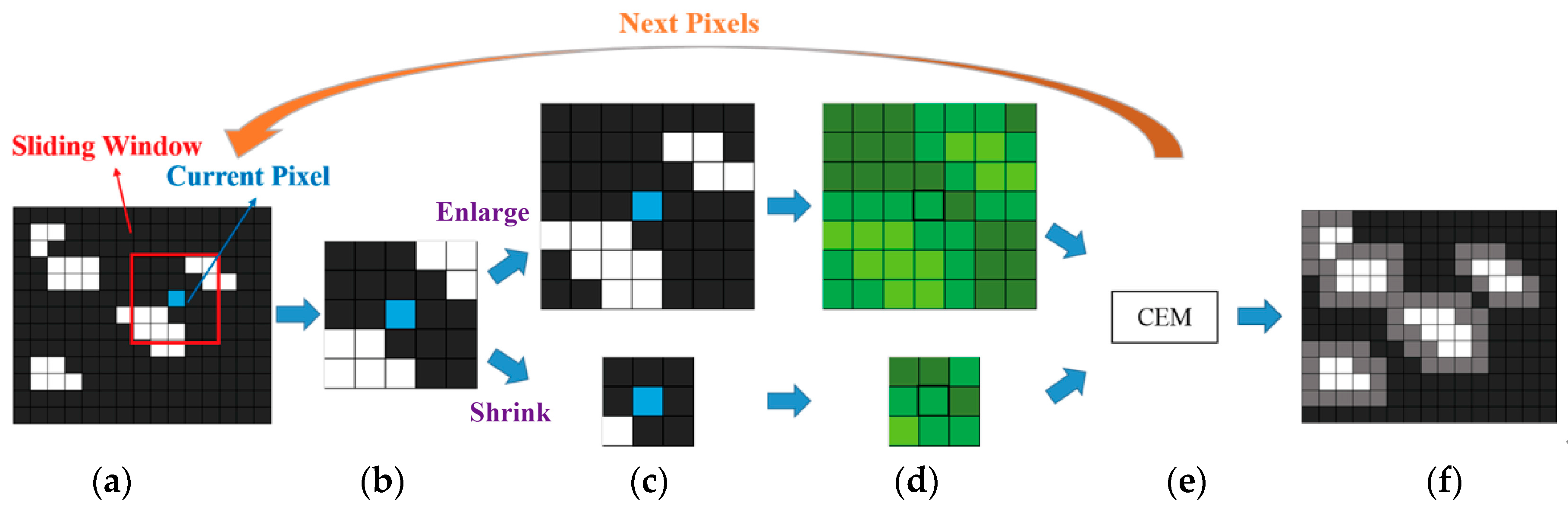
Flowchart of Adaptive Sliding Window CEM: (a) extract the newly grown leaves (NGL) around the current pixel from the preliminarily estimated sprout distribution map; (b) calculate the proportion of NGL in the sliding window; (c) enlarge or shrink the sliding window according to the proportion of NGL; (d) extract the pixel values from the window in relative position of the original image; (e) calculate the autocorrelation matrix for the pixel values in the window and substitute it in CEM for calculation; if all pixel values in the image are not finished, calculate the next pixel; and, (f) export the result of all pixel values.
Figure 7.
Flowchart of Adaptive Sliding Window CEM: (a) extract the newly grown leaves (NGL) around the current pixel from the preliminarily estimated sprout distribution map; (b) calculate the proportion of NGL in the sliding window; (c) enlarge or shrink the sliding window according to the proportion of NGL; (d) extract the pixel values from the window in relative position of the original image; (e) calculate the autocorrelation matrix for the pixel values in the window and substitute it in CEM for calculation; if all pixel values in the image are not finished, calculate the next pixel; and, (f) export the result of all pixel values.

Figure 8.
Flowchart of Optimal Signature Generation Process (OSGP).

Figure 9.
Flowchart of all algorithms for this experiment.

Figure 10.
Study site at Baihe District, Tainan, Taiwan.

Figure 11.
1000 × 1300 actual images of a forest in central Taiwan: (a) actual image of Region 1; and, (b) actual image of Region 2.
Figure 11.
1000 × 1300 actual images of a forest in central Taiwan: (a) actual image of Region 1; and, (b) actual image of Region 2.

Figure 12.
1000 × 1300 Groundtruth of forest in central Taiwan: (a) Groundtruth of Region 1 in the original picture; (b) Groundtruth of Region 2 in the original picture.
Figure 12.
1000 × 1300 Groundtruth of forest in central Taiwan: (a) Groundtruth of Region 1 in the original picture; (b) Groundtruth of Region 2 in the original picture.

Figure 13.
ROC Curve.

Figure 14.
Detection maps of 4 algorithms in Region 1. (a) CEM (b) Subset CEM (c) Sliding Window-based CEM (SW CEM) (d) Adaptive Window-based CEM (ASW CEM).
Figure 14.
Detection maps of 4 algorithms in Region 1. (a) CEM (b) Subset CEM (c) Sliding Window-based CEM (SW CEM) (d) Adaptive Window-based CEM (ASW CEM).

Figure 15.
Detection results highlighted with different colors of 4 algorithms in Region 1. (a) CEM (b) Subset CEM (c) Sliding Window-based CEM (SW CEM) (d) Adaptive Window-based CEM (ASW CEM).
Figure 15.
Detection results highlighted with different colors of 4 algorithms in Region 1. (a) CEM (b) Subset CEM (c) Sliding Window-based CEM (SW CEM) (d) Adaptive Window-based CEM (ASW CEM).

Figure 16.
Detection maps of 4 algorithms in Region 2. (a) CEM (b) Subset CEM (c) Sliding Window-based CEM (SW CEM) (d) Adaptive Window-based CEM (ASW CEM).
Figure 16.
Detection maps of 4 algorithms in Region 2. (a) CEM (b) Subset CEM (c) Sliding Window-based CEM (SW CEM) (d) Adaptive Window-based CEM (ASW CEM).

Figure 17.
Detection results highlighted with different colors of 4 algorithms in Region 2. (a) CEM (b) Subset CEM (c) Sliding Window-based CEM (SW CEM) (d) Adaptive Window-based CEM (ASW CEM).
Figure 17.
Detection results highlighted with different colors of 4 algorithms in Region 2. (a) CEM (b) Subset CEM (c) Sliding Window-based CEM (SW CEM) (d) Adaptive Window-based CEM (ASW CEM).

Figure 18.
ROC curves of local and global CEMs on Region 1.

Figure 19.
ROC curves of local and global CEMs on Region 2.

Figure 20.
Area under curve (AUC) detection results of Region 1 and Region 2.

Figure 21.
Kappa detection results of Region 1 and Region 2.

Figure 22.
Resulting images of the region where a false alarm is likely to occur in Region 1: (a) Traditional CEM; (b) Subset CEM; (c) SW CEM; (d) ASW CEM.
Figure 22.
Resulting images of the region where a false alarm is likely to occur in Region 1: (a) Traditional CEM; (b) Subset CEM; (c) SW CEM; (d) ASW CEM.

Figure 23.
Resulting images of the region where a false alarm is likely to occur in Region 2: (a) Traditional CEM; (b) Subset CEM; (c) SW CEM; and, (d) ASW CEM.
Figure 23.
Resulting images of the region where a false alarm is likely to occur in Region 2: (a) Traditional CEM; (b) Subset CEM; (c) SW CEM; and, (d) ASW CEM.

Figure 24.
Iterative process of OSGP and corresponding AUC detection result.

Figure 25.
AUC detection results of various algorithms executing five different d and corresponding d’ generated by OSGP (a) CEM; (b) Subset CEM; (c) SW CEM; and, (d) ASW CEM.
Figure 25.
AUC detection results of various algorithms executing five different d and corresponding d’ generated by OSGP (a) CEM; (b) Subset CEM; (c) SW CEM; and, (d) ASW CEM.

Figure 26.
RGB signatures corresponding to different objects in Region 1 [4].
Figure 26.
RGB signatures corresponding to different objects in Region 1 [4].

Figure 27.
RGB signatures with different objects in Region 2 [4].
Figure 27.
RGB signatures with different objects in Region 2 [4].


Table 1.
Parameter settings of different algorithms.
| Algorithm | Input Desired Target | Autocorrelation Matrix R | OGSP Stopping Rule | NGL Rate |
|---|---|---|---|---|
| Traditional CEM | d/d’ | Global R | θ | |
| Subset CEM | d/d’ | Local R (Fixed window size) | θ | |
| SW CEM | d/d’ | Local R (Fixed window size) | θ | |
| ASW CEM | d/d’ | Local R (Adaptive window size) | θ | ε |
Table 2.
Rates of Sprout and Non-Sprout in the ground truth.
| Image | Sprout | Non-Sprout | ||
|---|---|---|---|---|
| Pixels | Rate | Pixels | Rate | |
| Region 1 | 49,427 | 3.80% | 1,250,573 | 96.20% |
| Region 2 | 55,140 | 4.24% | 1,244,860 | 95.76% |
Table 3.
Error Matrix of Cohen’s kappa.
| Error Matrix | Ground Truth | Total | ||
|---|---|---|---|---|
| Sprout (p) | Non-Sprout (n) | |||
| Detection | Sprout (p’) | True Positive | False Positive | |
| Non-Sprout (n’) | False Negative | True Negative | ||
| Total | Total Pixels | |||
Table 4.
Detection results of traditional CEM and our proposed CEMs in the image of Region 1.
| Detection | AUC | PD | PF | ACC | Kappa |
|---|---|---|---|---|---|
| Traditional CEM | 0.9556 | 0.8794 | 0.1114 | 0.8882 | 0.3345 |
| Subset CEM | 0.9714 | 0.9122 | 0.0789 | 0.9207 | 0.4347 |
| SW CEM | 0.9737 | 0.9190 | 0.0723 | 0.9274 | 0.4604 |
| Adaptive-SW CEM | 0.9755 | 0.9299 | 0.0676 | 0.9323 | 0.4822 |
Table 5.
Detection results of traditional CEM and our proposed CEMs in the image of Region 2.
| Detection | AUC | PD | PF | ACC | Kappa |
|---|---|---|---|---|---|
| Traditional CEM | 0.9510 | 0.8952 | 0.1237 | 0.8771 | 0.3377 |
| Subset CEM | 0.9596 | 0.9099 | 0.0999 | 0.9005 | 0.3981 |
| SW CEM | 0.9649 | 0.9133 | 0.0885 | 0.9116 | 0.4310 |
| Adaptive-SW CEM | 0.9653 | 0.9212 | 0.0848 | 0.9155 | 0.4456 |
Table 6.
Detection results of Subset CEM with various window sizes.
| Subset CEM Window Size | AUC | PD | PF | ACC | Kappa |
|---|---|---|---|---|---|
| 50 × 65 | 0.9688 | 0.9108 | 0.0770 | 0.9227 | 0.4424 |
| 200 × 260 | 0.9714 | 0.9122 | 0.0789 | 0.9207 | 0.4347 |
| 500 × 650 | 0.9674 | 0.9048 | 0.0923 | 0.9075 | 0.3912 |
Table 7.
Detection results of SW CEM with various window sizes.
| SW CEM Window Size | AUC | PD | PF | ACC | Kappa |
|---|---|---|---|---|---|
| 101 × 101 | 0.9732 | 0.9179 | 0.0706 | 0.9290 | 0.4667 |
| 151 × 151 | 0.9737 | 0.9190 | 0.0723 | 0.9274 | 0.4604 |
| 301 × 301 | 0.9697 | 0.9135 | 0.0863 | 0.9137 | 0.4121 |
Table 8.
Computing time of different algorithms and CEM evaluation.
| Detection | Time | AUC Increment Rate | PD Increment Rate | PF Sink Rate | ACC Increment Rate | Kappa Increment Rate |
|---|---|---|---|---|---|---|
| Traditional CEM | 0.08 | 0.00% | 0.00% | 0.00% | 0.00% | 0.00% |
| Subset CEM | 0.08 | 1.22% | 2.38% | 2.82% | 2.80% | 8.03% |
| SW CEM | 326.24 | 1.60% | 2.89% | 3.72% | 3.69% | 10.96% |
| Adaptive-SW CEM | 232.33 | 1.71% | 3.83% | 4.14% | 4.13% | 12.78% |
© 2018 by the authors. Licensee MDPI, Basel, Switzerland. This article is an open access article distributed under the terms and conditions of the Creative Commons Attribution (CC BY) license (http://creativecommons.org/licenses/by/4.0/).
Share and Cite
MDPI and ACS Style
Chen, S.-Y.; Lin, C.; Tai, C.-H.; Chuang, S.-J. Adaptive Window-Based Constrained Energy Minimization for Detection of Newly Grown Tree Leaves. Remote Sens. 2018, 10, 96. https://doi.org/10.3390/rs10010096
AMA Style
Chen S-Y, Lin C, Tai C-H, Chuang S-J. Adaptive Window-Based Constrained Energy Minimization for Detection of Newly Grown Tree Leaves. Remote Sensing. 2018; 10(1):96. https://doi.org/10.3390/rs10010096
Chicago/Turabian StyleChen, Shih-Yu, Chinsu Lin, Chia-Hui Tai, and Shang-Ju Chuang. 2018. "Adaptive Window-Based Constrained Energy Minimization for Detection of Newly Grown Tree Leaves" Remote Sensing 10, no. 1: 96. https://doi.org/10.3390/rs10010096
Note that from the first issue of 2016, this journal uses article numbers instead of page numbers. See further details here.