Bayesian Cloud Detection for 37 Years of Advanced Very High Resolution Radiometer (AVHRR) Global Area Coverage (GAC) Data

Abstract

Cloud detection is a source of significant errors in retrieval of sea surface temperature (SST). We apply a Bayesian cloud detection scheme to 37 years of Advanced Very High Resolution Radiometer (AVHRR) Global Area Coverage (GAC) data, which is an important source of multi-decadal global SST information. The Bayesian scheme calculates a probability of clear-sky for each image pixel, conditional on the satellite observations and prior probability. We compare the cloud detection performance to the operational Clouds from AVHRR Extended algorithm (CLAVR-x), as a measure of improvement from reduced cloud-related errors. To do this we use sea surface temperature differences between satellite retrievals and in situ observations from drifting buoys and the Global Tropical Moored Buoy Array (GTMBA). The Bayesian scheme reduces the absolute difference between the mean and median SST biases and reduces the standard deviation of the SST differences by ~10% for both daytime and nighttime retrievals. These reductions are indicative of removing cloud contaminated outliers in the distribution, as these fall only on one side of the distribution forming a cold tail. At a probability threshold of 0.9 typically used to determine a binary cloud mask for SST retrieval, the Bayesian mask also reduces the robust standard deviation by ~5–10% during the day, in comparison with the operational cloud mask. This shows an improvement in the central distribution of SST differences for daytime retrievals.

1. Introduction

Remote sensing techniques are commonly used to retrieve geophysical properties of the Earth’s atmosphere and surface. For the majority of applications using data at thermal infrared wavelengths, classification of observations into clear or cloudy skies is a fundamental preprocessing step. Cloud detection methods can be used either to isolate clouds for retrieval of cloud properties, e.g., cloud optical depth, cloud top height [1,2], or for identifying and discarding regions where cloud obscures the Earth’s surface, essential for retrieval of surface parameters such as temperature, land cover classification and ocean colour [3,4,5,6].

Different approaches to image classification and cloud detection have been developed. One of the first approaches used to address the cloud detection problem (still commonly used) is to apply a series of threshold tests to the satellite imagery, based either on single channel properties, e.g., radiance, reflectance or brightness temperature, or using channel differences, normalised differences or textural measurements [7,8,9]. Typically, appropriate thresholds are determined using a selection of test data or case studies, and thresholds appropriate for one cloud type or atmospheric regime may not generalise well to other observation conditions.

This concept of applying a series of threshold-based tests to the observed data has been extended in the development of ‘fuzzy logic’ and neural networks for cloud detection. In these approaches binary thresholds are replaced with gradated boundaries defined using a cloud/clear weighting between 0–1. The outcomes of these tests are then combined, using a series of logical comparisons to give a final classification [10,11]. These logic models are developed using training data where the true classification of each observation is previously determined. Although neural networks may show good cloud detection skill under certain conditions, they are limited by the range of observations included in the training dataset.

A third approach is to use Bayes Theorem to determine a clear-sky probability given both the satellite observations and prior information on the background state [5,12]. We would expect this to be the optimum approach, as essentially cloud detection is a Bayesian problem, requiring an estimate of clear-sky probability given both satellite observations and prior knowledge of the surface conditions. In Bayesian approaches, this prior information is dynamic rather than static, increasing generality to a wide range of atmospheric conditions. A threshold can then be placed on this probability to determine a binary cloudmask appropriate to the application. In some retrieval algorithms a naive Bayesian approach is used assuming independence between classifiers (i.e., different channels or cloud tests) [13,14]. This can considerably reduce the size of the probability density space used to describe each classifier, and is often used to reduce the complexity of the problem or increase data processing speed. Arguably, however, the main benefit of a full Bayesian approach to cloud-screen multi-channel data comes from coherent assessment of joint probability distributions, as in reality individual classifiers are not independent.

Comparison studies have provided evidence that Bayesian techniques can more succesfully detect cloud under a range of different meteorological conditions than threshold-based methodologies [3,5]. Further, Bayesian approaches have been applied to retrievals of sea surface temperature [5,15] with their potential for use at high latitudes and over land also demonstrated [3,12]. Within the context of the European Space Agency’s (ESA) Sea Surface Temperature Climate Change Initiative (SST CCI) and ATSR Reprocessing for Climate (ARC) projects, full Bayesian methods are applied to the dual-view Along Track Scanning Radiometer instruments [15,16] in the production of climate data records.

In this paper we consider the application of Bayesian methods to the Advanced Very High Resolution Radiometers (AVHRRs), assessing cloud detection skill against a heritage cloud mask provided in operational products. The paper is structured as follows: in Section 2 we describe the Bayesian cloud detection and its application to AVHRR, detailing the relevant instrument characteristics. In Section 3 we describe the application of single-sensor look-up tables to other instruments in the AVHRR data record, and in Section 4 we validate the cloud mask performance using SST comparison statistics and discuss the results. We conclude the paper in Section 5.

2. Bayesian Cloud Detection for AVHRR

Bayesian cloud detection methods as a pre-processing step for sea surface temperature (SST) retrieval have been used extensively with the Along-Track Scanning Radiometers (ATSRs) in the provision of SST data for climate applications [15,16]. The Bayesian methodology for cloud detection is described in detail in [5] and outlined only briefly here as this paper focuses on the applicability to data from the AVHRR sensors. The probability of clear-sky $P(c|{\mathbf{y}}^{\mathbf{o}},{\mathbf{x}}^{\mathbf{b}})$ given both the observation vector ${\mathbf{y}}^{\mathbf{o}}$ and prior knowledge of the background state ${\mathbf{x}}^{\mathbf{b}}$ is:

$$P(c|{\mathbf{y}}^{\mathbf{o}},{\mathbf{x}}^{\mathbf{b}})={[1+\frac{P\left(\overline{c}\right)P({\mathbf{y}}^{\mathbf{o}}|{\mathbf{x}}^{\mathbf{b}},\overline{c})}{P\left(c\right)P({\mathbf{y}}^{\mathbf{o}}|{\mathbf{x}}^{\mathbf{b}},c)}]}^{-1}$$

(1)

where the observation vector consists of the satellite observations and the background state vector includes the prior sea surface temperature, total column water vapour and windspeed from the ERA-Interim numerical weather prediction (NWP) data [17]. $P\left(\overline{c}\right)$ and $P\left(c\right)$ are the prior probabilities of cloudy and clear skies defined using the total cloud cover in the NWP data (where $\overline{c}$ and c denote cloud and clear conditions respectively). Limits are placed on these estimates that prevent the prior probability of cloud exceeding 95% or falling below 50%. These limits ensure that the cloud prior probability is both realistic and that the prior probability of cloud is not set to 100%. $P({\mathbf{y}}^{\mathbf{o}}|{\mathbf{x}}_{\mathbf{b}})$ is the probability of the observations given the background state summed over clear and cloudy conditions, specified using an emprical look-up table for cloudy conditions (Section 2.4) and simulated using a radiative transfer model for clear-sky conditions (Section 2.3). Error covariance matrices used in the Bayesian calculation include terms for noise in the observations, uncertainty in the prior and forward model uncertainty.

2.1. Advanced Very High Resolution Radiometer Data

The Advanced Very High Resolution Radiometer (AVHRR) instrument comes in three different configurations. The AVHRR-1 instrument has the smallest compliment of channels at 0.6, 0.8, 3.7 and 10.8 $\mathsf{\mu }$m. The AVHRR-2 instrument has an additional 12 $\mathsf{\mu }$m channel and the AVHRR-3 instrument includes a 1.6 $\mathsf{\mu }$m channel, which can be switched with the 3.7 $\mathsf{\mu }$m channel on command. AVHRR data are available at two different resolutions. Full resolution data are 1.1 km at the sub-satellite point, and only routinely provided globally for the MetOp series of sensors. For earlier sensors, data are provided at a nominal resolution of 4 km at the sub-satellite point, and this data stream is referred to as ‘global area coverage’ (GAC) data. GAC data are derived by sampling four pixels across-track, missing one, and then sampling the next four, in every third scanline. The GAC data transmitted from the satellite are then an average of the signal across each four pixel block, and represent the geographical area of 3 × 5 full resolution pixels [18]. The first AVHRR instrument was TIROS-N, launched in 1978, and the AVHRR series provide an unbroken record of Earth observations over a 39 year time period, a data record length ideal for climate applications. Here we consider the data record from AVHRR-06 launched in 1979 through to MetOp-A at the end of 2016.

Table 1. AVHRR instrument record indicating instrument name and type, period of operation, channel availability and daytime equator overpass time. Parenthesis around a given channel indicates that data from that channel are not routinely transmitted.

Instrument	Type	Period of Operation	Channel Availability ($\mathsf{\mu }$m)	Overpass Time
NOAA-6	AVHRR-1	July 1979–March 1982	0.6, 0.8, 3.7, 10.8	Morning
NOAA-7	AVHRR-2	September 1981–February 1985	0.6, 0.8, 3.7, 10.8, 12.0	Afternoon
NOAA-8	AVHRR-1	May 1983–October 1985	0.6, 0.8, 3.7, 10.8	Morning
NOAA-9	AVHRR-2	February 1985–November 1988	0.6, 0.8, 3.7, 10.8, 12.0	Afternoon
NOAA-10	AVHRR-1	November 1986–September 1991	0.6, 0.8, 3.7, 10.8	Morning
NOAA-11	AVHRR-2	November 1988–December 1994	0.6, 0.8, 3.7, 10.8, 12.0	Afternoon
NOAA-12	AVHRR-2	September 1991–December 1998	0.6, 0.8, 3.7, 10.8, 12.0	Morning
NOAA-14	AVHRR-2	January 1995–October 2002	0.6, 0.8, 3.7, 10.8, 12.0	Afternoon
NOAA-15	AVHRR-3	October 1998–December 2010	0.6, 0.8, (1.6), 3.7, 10.8, 12.0	Morning
NOAA-16	AVHRR-3	January 2001–December 2010	0.6, 0.8, (1.6), 3.7, 10.8, 12.0	Afternoon
NOAA-17	AVHRR-3	June 2002–December 2010	0.6, 0.8, 1.6, 3.7, 10.8, 12.0	Morning
NOAA-18	AVHRR-3	May 2005–Present	0.6, 0.8, (1.6), 3.7, 10.8, 12.0	Afternoon
NOAA-19	AVHRR-3	February 2009–Present	0.6, 0.8, (1.6), 3.7, 10.8, 12.0	Afternoon
MetOp-A	AVHRR-3	October 2006–Present	0.6, 0.8, 1.6, 3.7, 10.8, 12.0	Morning

provides a list of the AVHRR instruments, their period of operation (note that for earlier sensors there may be data gaps within this record), available channels and equator overpass time.

2.2. AVHRR Level 1 Calibration and Harmonisation

When considering long time series of data covering observations from multiple sensors, both the accuracy of individual sensor calibration and the biases between sensors are important. Instrument calibration can change over time due to sensor degredation, and individual sensors may show biases in relation to a reference sensor. In this section, we discuss how we address these issues for both the visible and infrared channels.

2.2.1. Visible Channels

For the AVHRR instruments there is no on-board calibration system to track any changes in the visible channel detector response but it is now known that significant instrument degradation over time has occurred e.g., [19]. From November 1996, the National Oceanographic and Atmospheric Administration (NOAA) has provided an operational monthly update to the visible channel coefficients based on the Libya-4 desert reference site [19]. However, data prior to November 1996 have not been corrected, and therefore the visible degradation can affect the cloud detection which could result in spurious trends in SST.

To remove these calibration trends and improve the visible channel data, there are several recalibration schemes available. Along with the operational updates discussed above, coefficients are available from the Community Satellite Processing Package (CSPP) software available from the Co-operative Institute for Meteorological Satellite Studies (CIMSS) (based on the Heidinger et al. algorithm [20]), from the NASA Langley Research Centre (LaRC) AVHRR Fundamental Climate Data Record (FCDR) project, from the NOAA Climate Data Record Program (e.g., [21]), from the University of Maryland (e.g., [22]) and others. The most recent of these are based on a number of different references including MODIS channels, desert sites, cloud tops and sites such as Dome-C in the Antarctic. In general, they have quoted accuracies of the order of 2–3%.

In the ESA SST CCI project we have used the CSPP coefficients (dated to late 2015) to calibrate the visible channels. These coefficients provide a time dependent model for the calibration coefficients based on time from launch. Beyond the update to the calibration coefficients we have also used a simple outlier rejection scheme to remove spurious counts from the space view data and have applied the same smoothing kernel to the space view data as is used for the IR calibration (see Section 2.2.2). These two extra processing steps will result in slightly different values than would be provided by the CSPP software directly but should improve stability.

2.2.2. Infrared Channels

The AVHRR has up to three IR channels and has an internal calibration target (ICT) which is used to determine variations in the instrument gain. To improve the calibration signal-to-noise we first use smoothed values of the calibration counts (space view and ICT view) and the ICT temperatures. Then to calibrate the IR channels we use the Walton et al. calibration algorithm [23] (the current operational calibration) using calibration coefficients taken from the CSPP. This is because the CSPP has coefficients for all the AVHRR sensors including coefficients for the AVHRR-1 instruments that do not have a 12 $\mathsf{\mu }$m channel (NOAA-06, NOAA-08 and NOAA-10), which were not included in the original analysis [23]. To calibrate the IR channels, we first assume that the 3.7 $\mathsf{\mu }$m channel is completely linear so the gain can be simply calculated from the calibration observations. The 10.8 $\mathsf{\mu }$m and 12 $\mathsf{\mu }$m channels are, however, known to be non-linear and the calibration first derives a linear radiance (including a bias correction term called the ‘negative radiance of space’) and then uses a quadratic based on this linear radiance as a non-linear correction term.

At this point, we note that all the calibration coefficients in the operational calibration [23] were based on an analysis of the pre-launch data which has subsequently been shown to have numerous problems ([24]) and are therefore suspect. Further, the difference between the thermal environment of the pre-launch testing (where uniform temperature gradients were a goal) and the thermal environment in-orbit (where directional heating from the Sun will cause strong thermal gradients) will impact the calibration. This variation in thermal gradients is particularly important when considering the long-term stability of the instrument because most of the AVHRRs are not in stable orbits but are in orbits that drift (see Figure 1), thereby varying the thermal state of the AVHRR on long timescales.

Biases in the operational IR AVHRR radiances [23] have been previously reported. For example, a strong (up to 0.5 K) scene temperature dependent bias has been seen in the AVHRRs flown on-board the MetOp series of satellites (e.g., [25,26]) and there is also evidence for a large time dependent bias due to changes in the AVHRR thermal state (e.g., [25,27]). To take both these sources of bias into account we have therefore implemented a two-step bias correction scheme applied to the operational calibration. We first determine the AVHRR bias relative to clear-sky radiances over ocean scenes (estimated using the ERA Interim atmospheric profiles together with RTTOV v11.3 as the radiative transfer model). Because there is a distinct lack of temperature sensors on the AVHRR (for the early sensors there are just the ICT PRT temperatures available) we have to estimate the AVHRR thermal state using the orbital average of the ICT temperature as a proxy. Then to model the bias we use a range of different model types such as simple polynomials and two state linear models (where there is a clear difference between trends as a function of orbital averaged ICT temperature). Different models are applied for different time periods all as a function of the orbital average ICT temperature. Full details of the time dependent biases seen in the AVHRR will be presented elsewhere.

Once the time dependent bias has been corrected for we then use the overlap period of the AVHRRs with the (A)ATSR sensors to determine an average scene temperature dependent bias. To ensure compatibility with the thermal state dependent bias discussed above we have again taken just the clear-sky matches between the AVHRR and (A)ATSR sensors. We have then used a double difference method (e.g., [28]) between the AVHRR and (A)TSR sensors which allows for large time separation in the matches (of order hours) as well as automatically correcting for spectral response function differences between sensors. A single linear fit of bias as a function of scene temperature was then made to all the (A)ATSR/AVHRR matchups which effectively links all the AVHRR sensors to the (A)ATSR sensors as a reference. Note that by fitting to all the overlapping sensors simultaneously we are also trying to capture the range of error in the calibration across all sensors and the standard deviation seen around the bias model is added to the total uncertainty of the IR calibration. For those sensors which do not overlap the (A)ATSR period we then double this uncertainty in an effort to take the lack of a reference pre-1995 (pre ATSR-2) into account.

Finally, an estimate of the radiance uncertainty for each pixel is derived from the counts noise seen in the space view coupled with the estimated instrument gain. To this we add the calibration uncertainty defined above and the total radiance uncertainty is converted into an noise equivalent differential temperature (NEdT, defined for a scene temperature of 300 K) for use with subsequent processing.

2.3. Simulating Clear-Sky Observations

For clear-sky conditions we use the fast forward radiative transfer model RTTOV v11.3, which has the ability to simulate top-of-atmosphere radiances at both visible and infrared wavelengths [29]. We have used infrared channel simulations extensively in previous applications of the Bayesian cloud screening to ATSR data [5,16] but here use similar information from the 0.6 and 0.8 $\mathsf{\mu }$m visible wavelength channels in daytime cloud detection. RTTOV v11.3 radiative transfer is coupled with a Cox and Munk parameterisation of surface reflectance and glint [30], to determine suitability for cloud detection purposes. We compare simulated and observed reflectance in the 0.6 and 0.8 $\mathsf{\mu }$m channels using an SST match-up database [31] including all AVHRR sensors used in the data record. Clear-sky matches were selected using Bayesian cloud detection with infrared channels only, including checks for bad data, navigation and calibration problems. Although the Bayesian cloud detection using only the 10.8 and 12 $\mathsf{\mu }$m channels is not perfect, averaging the reflectances within radiative transfer model (RTM) reflectance bins minimises the impact of missed clouds on the resulting fit. 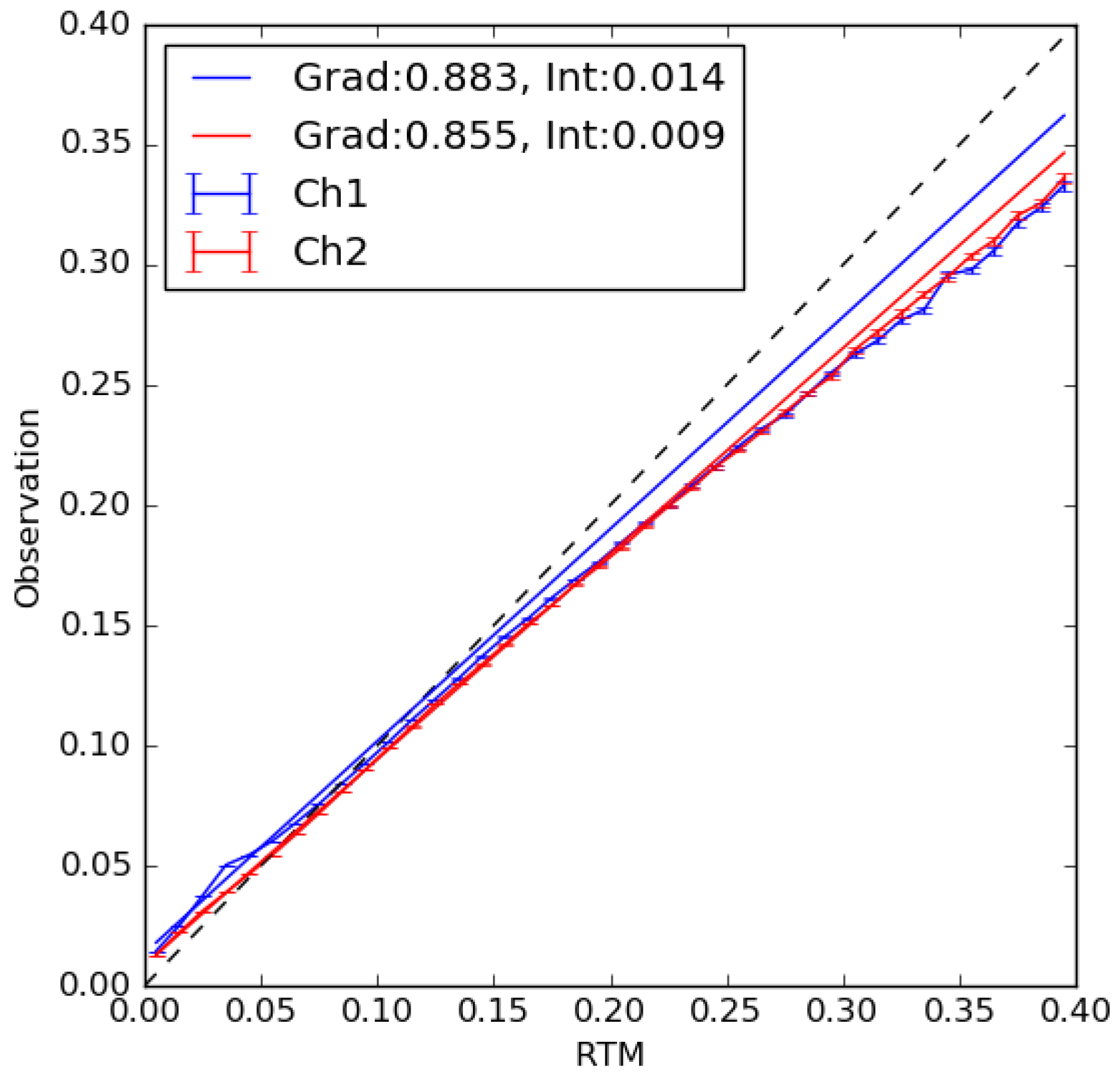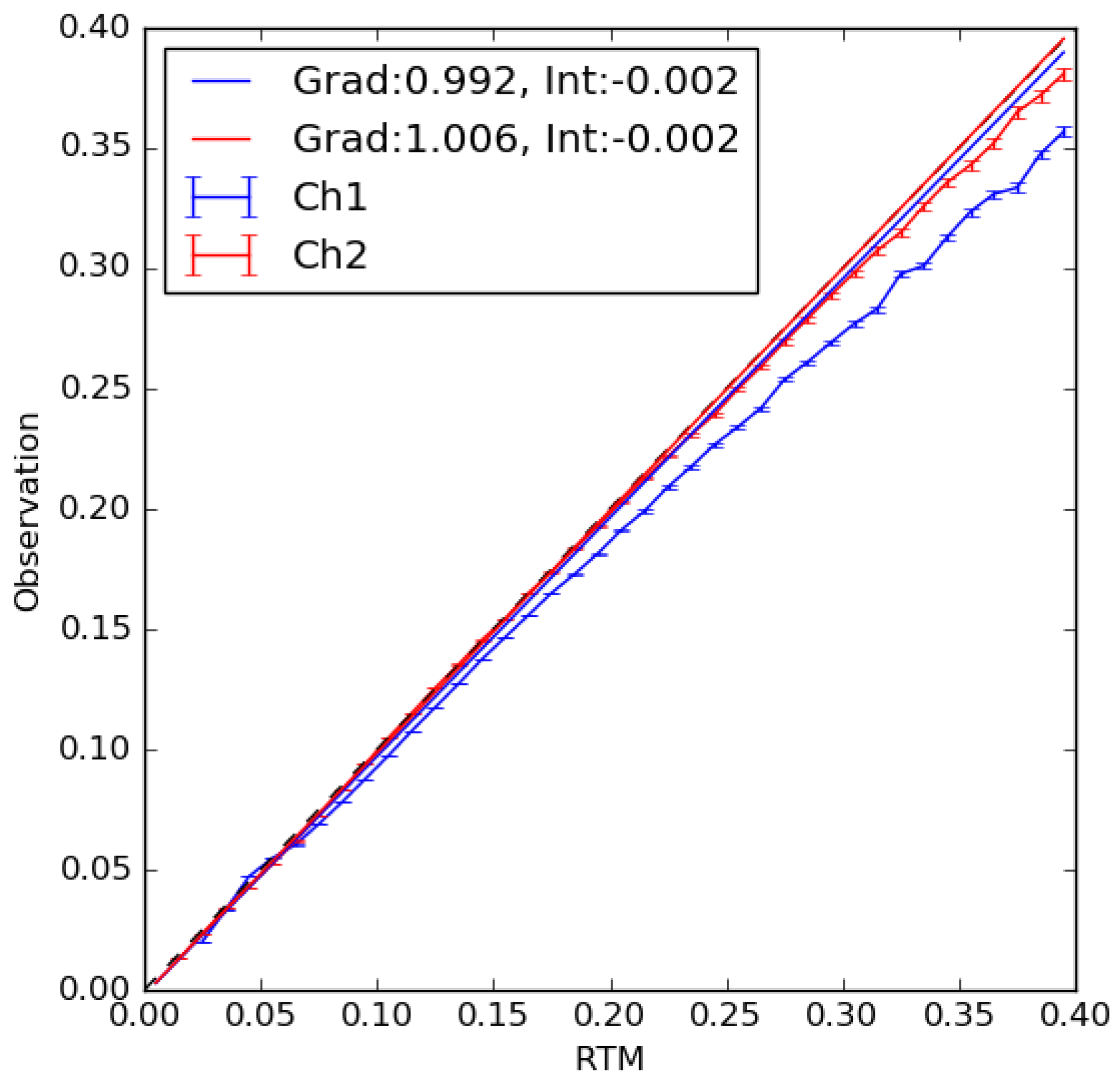Figure 2 shows the 0.6 and 0.8 $\mathsf{\mu }$m data plotted in bins of 0.01 RTM reflectance including a linear regression for each channel. RTTOV v11.3 overestimates reflectance under brighter conditions compared to the observations in both channels. We therefore apply a simple linear correction to the RTTOV v11.3 simulations when processing the AVHRR data to align them more closely with the observations. A single correction is applied uniformly to all AVHRR sensors (similar results were found when considering each sensor individually but are not shown here), and Figure 3 shows a comparison for RTM minus observation for clear-sky matches with the correction applied. Linear regressions for both channels now lie almost directly along the 1:1 line, with a small deviation of the data at high reflectance. Most clear-sky observations have reflectance below 0.2 and in those regions these simulations are now accurate enough to use in the cloud detection scheme. Performance of the classifier under sunglint conditions, where the top of atmosphere reflectance will be higher, is specifically addressed in Section 4.

2.4. Empirical Cloudy PDFs

To calculate the probability of clear-sky, we need to determine the probability of the observations given the background state $P({\mathbf{y}}^{\mathbf{o}}|{\mathbf{x}}_{\mathbf{b}})$ under both clear-sky and cloudy conditions. For cloudy conditions, simulating top of atmosphere radiances on-the-fly is computationally expensive. We therefore represent cloudy observations using pre-calculated empirical probability density functions (PDFs) derived from MetOp-A GAC data between 2006–2017. We generate the PDFs using a single iteration of our Bayesian cloud detection algorithm, bootstrapped using empircal cloudy PDFs for the Advanced Along Track Scanning Radiometer (AATSR) cloud detection. We use a brightness temperature shift at the point of indexing the look-up table to make the AVHRR observations ‘look like’ AATSR (the methodology is described in detail in Section 3). Further, as AATSR makes observations in two views (satellite zenith angles of 0${}^{\circ }$–22${}^{\circ }$ in the nadir and 52${}^{\circ }$–55${}^{\circ }$ degrees in the forward view), the AATSR PDFs are interpolated as a function of path length to represent the other viewing angles seen by MetOp-A. We also note that although the AVHRR GAC data does come with an operational cloud mask (CLAVR-x), we found that the performance of this mask was insufficient to prevent inclusion of large numbers of clear-sky observations in the empirical PDFs, rendering this unsuitable for bootstrapping the PDF generation.

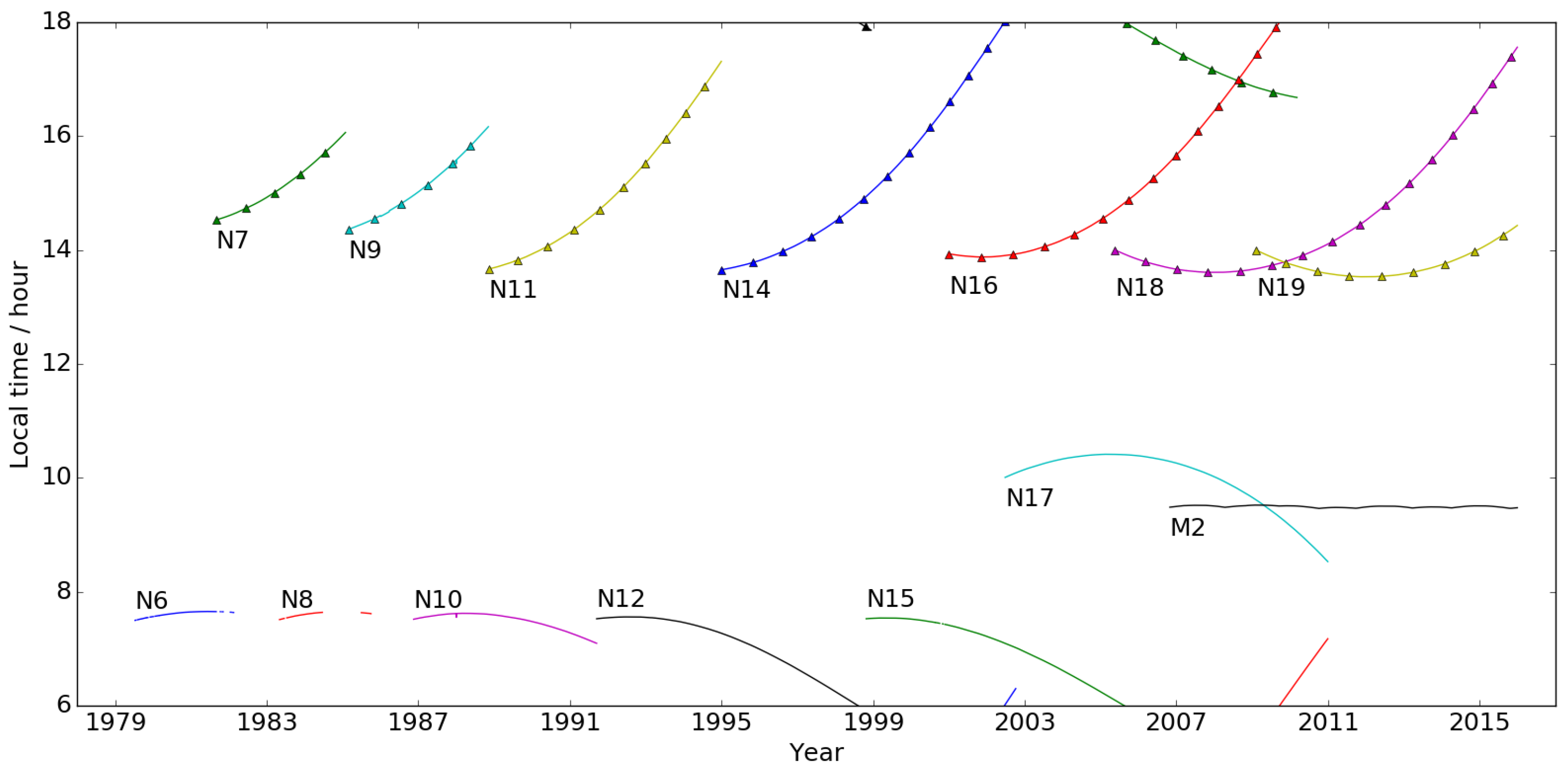
Figure 1 shows daytime equator overpass times for all of the AVHRR sensors. Metop-A was selected as the baseline for creating the AVHRR cloudy PDFs due to the orbital stability. It is one of the few AVHRR instruments which does not show significant orbital drift over time, it has the maximum number of channels available for AVHRR instruments, and has a long data record spanning 10 years.

Table 2. Empirical cloudy PDF specifications as applied for AVHRR cloud detection. Acronyms used are as follows: BT - brightness temperature, NWP - numerical weather prediction, SST - sea surface temperature, Diff - difference, SZA - solar zenith angle.

PDF	Sensor	Dimension	Lower Limit	Upper Limit	Bin Size	No. of Bins
Daytime Spectral PDF 1	1,2,3	0.6 $\mathsf{\mu }$m refl	0.0	1.0	0.01	100
		0.8 $\mathsf{\mu }$m refl	0.0	1.0	0.01	100
		SZA	0.0	95.0	2.5	38
		Path Length	1.0	2.4	0.35	4
Daytime Spectral PDF 2	2,3	10.8 $\mathsf{\mu }$m BT–NWP SST	−20.0	10.0	1.0	30
		10.8–12 $\mathsf{\mu }$m BT	−1.0	9.0	0.2	50
		NWP SST	260.0	310.0	1.0	50
		Path Length	1.0	2.4	0.35	4
		Day/Night	0.0	180.0	90.0	2
Daytime Spectral PDF 3	1	10.8 $\mathsf{\mu }$m BT	260.0	305.0	1.0	45
		NWP SST	260.0	310.0	1.0	50
		Path Length	1.0	2.4	0.35	4
		Day/Night	0.0	180.0	90.0	2
Nighttime Spectral PDF 1	2,3	10.8 $\mathsf{\mu }$m BT–NWP SST	−20.0	10.0	1.0	30
		10.8–12 $\mathsf{\mu }$m BT Diff	−1.0	9.0	0.2	50
		3.7–10.8 $\mathsf{\mu }$m BT Diff	−6.0	10.0	0.2	80
		NWP SST	260.0	310.0	2.5	20
		Path Length	1.0	2.4	0.35	4
		Day/Night	0.0	180.0	90.0	2
Nighttime Spectral PDF 2	1	10.8 $\mathsf{\mu }$m BT–NWP SST	−20.0	10.0	1.0	30
		3.7–10.8 $\mathsf{\mu }$m BT Diff	−6.0	10.0	0.2	80
		NWP SST	260.0	310.0	1.0	50
		Path Length	1.0	2.4	0.35	4
		Day/Night	0.0	180.0	90.0	2
Textural PDF	1,2,3	10.8 $\mathsf{\mu }$m BT	260.0	305.0	1.0	45
		NWP SST	260.0	310.0	1.0	50
		Path Length	1.0	2.4	0.35	4

describes the AVHRR PDF construction, where separate look-up tables are used for spectral and textural features. There are three spectral PDFs generated for processing daytime data, and two for nighttime data (labelled PDF 1, PDF 2, PDF 3 in Table 2). The PDFs used are dependent on the sensor, for example during the day, AVHRR -1 instruments use daytime spectral PDF 1 and PDF 3, while AVHRR-2/3 instruments use daytime spectral PDF 1 and PDF 2. A single textural PDF is used regardless of the time of day.

Spectral PDFs are generated under cloudy conditions only, while textural PDFs are calculated under both clear and cloudy conditions. In terms of individual PDFs, the visible channel spectral PDF 1 is used during the day and is applicable to all AVHRR instruments as it uses the 0.6 and 0.8 $\mathsf{\mu }$m channels only. For the infrared daytime PDF, we use the 10.8 and 12 $\mathsf{\mu }$m for AVHRR-2 and 3 instruments (daytime spectral PDF 2), and the 10.8 $\mathsf{\mu }$m only for AVHRR-1 (daytime spectral PDF 3) as the 12 $\mathsf{\mu }$m isn’t present. At night, the spectral PDFs are extended to include the shortwave infrared 3.7 $\mathsf{\mu }$m channel (nighttime spectral PDFs 1 and 2). Finally the textural PDF uses the local standard deviation of the 10.8 $\mathsf{\mu }$m brightness temperature over a 3 × 3 pixel domain, centred on the pixel to be classified. This PDF is used consistently under day and nighttime conditions, for all AVHRR sensors.

Given the equator overpass time of the sensor however, MetOp-A does not make observations at the full range of solar zenith angles observed by other AVHRR sensors with different equator overpass times, and consequently the visible channel PDFs need to be extended in order to be applicable to the entire data record. To do this, we use data from NOAA-18, which has an afternoon equator overpass time. Although still currently operational, NOAA-18 shows a step-change in the SST data record post-2010. We therefore use only observations made between 2005–2009. MetOp-A routinely makes observations in the solar zenith angle range 25${}^{\circ }$–90${}^{\circ }$ (with this range extending to smaller solar zenith angles at longer atmospheric path lengths). NOAA-18 routinely makes observations at solar zenith angles as low as 15${}^{\circ }$ at nadir, and in the range not observed by MetOp-A we use NOAA-18 data to directly fill the corresponding bins in the look-up table. For lower solar zenith angles than those observed by either instrument, we use the average of the first three valid bins from the NOAA-18 data to define the PDF. This approach can be justified as conditions for solar zenith angles of ~15${}^{\circ }$ are very similar to when the sun is directly overhead. These data will be relevant for AVHRR sensors that show significant orbital drift throughout their lifetime, deviating substantially from the equator overpass times represented by MetOp-A and NOAA-18.

2.5. High Latitude Ice Masking

In regions where there is a chance that the sea surface freezes, cloud masking has to be extended to also include sea-ice masking. Clouds and sea-ice do have some similar spectral signatures, but for other features, the spectral signature for sea-ice can be closer to cloud-free sea. Therefore sea-ice masking should be included in the classification when processing SST at high latitudes. One solution could be to extend the two-way classifier described at the start of Section 2 to a three-way classifier on a global scale. Another option is to include a classifier adapted for sea-ice masking in regions where sea ice can occur as we do here.

The sea-ice masking has been set up using a three-way classifier trained for high latitude areas, and therefore only to be applied at high latitudes. The idea is that all pixels classified as cloud free by the two-way classifier at high latitudes undergo an additional classification by a three-way classifier that also includes sea-ice. This is used to potentially reclassify clear-sky pixels as ‘not clear’ only, by reducing the probability of clear-sky given by the Bayesian calculation. The clear-sky probability is set to the minimum of the clear-sky probability given by the two-way classification, and the clear-sky probability given by the three-way classification.

High latitudes can be defined as areas poleward of 50 N/S, or more specifically as areas within the climatological maximum sea-ice extent. We use the latter to define sea-ice affected regions using monthly data from National Snow and Ice Data Center (NSIDC) [32] . The sea-ice edge has been extended by 100 km into the open water definition to account for the daily sea-ice edge fluctuations.

The three-way classifier is defined in a similar way as the two-way Bayesian classifier (1), except that a third ice covered class is added. The probability of a pixel being clear-sky over ocean in a n-way classifier is given in (2) [12], where class${}_n$ includes clear (c), cloud ($\overline{c}$) and ice (i):

$$P(c|{\mathbf{y}}^{\mathbf{o}},{\mathbf{x}}^{\mathbf{b}})=\frac{P\left(c\right)P({\mathbf{y}}^{\mathbf{o}}|{\mathbf{x}}^{\mathbf{b}},c)}{{\sum }_{n}P\left(clas{s}_n\right)P({\mathbf{y}}^{\mathbf{o}}|{\mathbf{x}}^{\mathbf{b}},clas{s}_n)}$$

(2)

For this work, the three-way classifier developed in the EUMETSAT Oceans and Sea Ice Satellite Application Facility (OSI SAF) project and SST CCI Phase 1 [12] has been used. This classifier has been trained on AVHRR GAC data to work for all sensors in the series. This training is necessary to define the PDFs for the three classes (clear, cloud, ice) and uses an empirical approach. To generate the PDFs, the EUMETSAT Climate SAF cLoud, Albedo and surface RAdiation dataset from AVHRR data (CLARA-A2) dataset [33] and the EUMETSAT OSI SAF CDR on sea ice concentration [34] have been used. CLARA-A2 consists of both re-calibrated AVHRR channel data and cloud/ice masking products. The cloud/ice mask from CLARA-A2 and OSI SAF sea ice concentration are used to define occurrence of cloud and ice, and this is used together with the CLARA-A2 satellite data to define the PDFs for all the AVHRR sensors. For each AVHRR sensor, three years of GAC data are used to define the PDFs.

The CLARA-A2 dataset does not contain any AVHRR-1 data. To define PDFs for NOAA-6, 8 and 10 the AVHRR-2 sensor which is closest in terms of spectral response functions has been used as a proxy (NOAA-7). The PDFs used for the high latitude ice masking are listed in

Table 3. Features used for three-way classification PDFs, dependent on AVHRR sensor and time of day. All PDFs are two dimensional with a feature and single dependency. The following acronyms are used: BT = brightness temperature, SZA = solar zenith angle, Atm = Atmospheric, Std = Standard Deviation, diff = difference, refl = reflectance.

PDF	Sensor	Feature	Dependencies	Range	Binsize
Daytime Spectral Feature 1	1,2,3	0.8/0.6 $\mathsf{\mu }$m refl ratio	SZA	0–91	1
Daytime Spectral Feature 2a ${}^{*}$	3	1.6/0.6 $\mathsf{\mu }$m refl ratio	SZA	0–91	1
Daytime Spectral Feature 2b	1,2,3	3.7–10.8 $\mathsf{\mu }$m BT diff	SZA	0–91	1
Daytime Spectral Feature 3	1,2,3	0.6 $\mathsf{\mu }$m reflectance	SZA	0–91	1
Nighttime Spectral Feature 1	1	3.7–10.8 $\mathsf{\mu }$m BT diff	Atm. Path Length	1–2.5	0.1
Nighttime Spectral Feature 2	2,3	10.8–12 $\mathsf{\mu }$m BT diff	3.7–12 $\mathsf{\mu }$m BT diff	−1.5–4	0.1
Nighttime Textural Feature 3a	2,3	Std(3.7–12 $\mathsf{\mu }$m BT)	Atm. Path Length	1–2.5	0.1
Nighttime Textural Feature 3b	1	Std(3.7–10.8 $\mathsf{\mu }$m BT)	Atm. Path Length	1–2.5	0.1

${}^{*}$ This feature is only used when the 1.6 $\mathsf{\mu }$m channel is available for AVHRR-3 instruments. Where this is unavailable, daytime spectral feature 2b is used.

. Some PDFs are the same for all AVHRRs, while others are only used for AVHRR-2 and/or 3. This is identified with an ‘a’ or ‘b’ in the PDF name, and in the column specifying the sensor.

3. Applying Metop-A Empirical PDFs to Other AVHRR instruments

In processing the AVHRR GAC archive, it is useful to be able to apply a single set of empirical PDFs to all instruments, providing consistency between sensors and minimising the use of disk space for storing ancillary data. In order to do this, we need to make observations from the sensor that is being processed closely match MetOp-A observations, by applying a brightness temperature shift at the point of indexing the look-up table. In order to calculate the shift required for each AVHRR instrument, we use RTTOV v11.3 to simulate clear-sky brightness temperatures for 2100 atmospheric profiles derived from ERA-40 [35,36]. These profiles are chosen to be representative of the variety of atmospheric conditions observed globally over the oceans, incorporating a range of surface temperatures, total column water vapour (TCWV) and ozone concentrations.

We run RTTOV v11.3 for each profile and each AVHRR instrument for two atmospheric path lengths: 1.0 and 1.8, corresponding to satellite viewing zenith angles of 0${}^{\circ }$and 56.25${}^{\circ }$, which covers the full range of angles observed by the AVHRR instruments (0${}^{\circ }$–55.37${}^{\circ }$) [18]. We calculate the difference between MetOp-A brightness temperatures and those from each of the other sensors in the 3.7, 10.8 and 12 $\mathsf{\mu }$m channels (subject to channel availability). Figure 4 shows these differences for each sensor as a function of TCWV. The raw data are plotted for the nadir view only, and the solid and dashed lines show the cubic fit to the difference for atmospheric path lengths of 1.0 and 1.8 respectively. For any given observation path length we linearly interpolate between these cubic fits to get coefficients corresponding to the observation. The coefficients for atmospheric path lengths of 1.0 and 1.8 are provided in

Table 4. Cubic coefficients for AVHRR MetOp-A minus AVHRR sensor differences simulated using RTTOV v11.3 for an atmospheric path length of 1.0. Coeffiecients are a function of total column water vapour.

Sensor	Channel	a0	a1	a2	a3
NOAA-19	3.7 $\mathsf{\mu }$m	−0.027	0.00016	−3.348 × 10${}^{-5}$	2.56 × 10${}^{-7}$
	10.8 $\mathsf{\mu }$m	−0.001	3.566 × 10${}^{-5}$	−2.275 × 10${}^{-5}$	1.289 × 10${}^{-7}$
	12 $\mathsf{\mu }$m	0.205	0.0115	−2.9109 × 10${}^{-5}$	−1.073 × 10${}^{-7}$
NOAA-18	3.7 $\mathsf{\mu }$m	0.0309	−0.00308	2.856 × 10${}^{-5}$	−4.6126 × 10${}^{-7}$
	10.8 $\mathsf{\mu }$m	−0.00896	0.000132	−2.0128 × 10${}^{-5}$	1.0472 × 10${}^{-7}$
	12 $\mathsf{\mu }$m	0.1309	0.00668	−2.45072 × 10${}^{-6}$	−2.127005 × 10${}^{-7}$
NOAA-17	3.7 $\mathsf{\mu }$m	−0.01939	−0.00034	−2.4193 × 10${}^{-5}$	1.5347 × 10${}^{-7}$
	10.8 $\mathsf{\mu }$m	−0.00015	−0.000258	−6.9899 × 10${}^{-6}$	2.3774 × 10${}^{-8}$
	12 $\mathsf{\mu }$m	−0.03096	2.44656 × 10${}^{-5}$	−1.9455 × 10${}^{-5}$	8.2992 × 10${}^{-8}$
NOAA-16	3.7 $\mathsf{\mu }$m	−0.3313	0.0127	−0.000315	3.357 × 10${}^{-6}$
	10.8 $\mathsf{\mu }$m	0.02097	0.000595	7.068 × 10${}^{-5}$	−2.9927 × 10${}^{-7}$
	12 $\mathsf{\mu }$m	0.11156	0.0079	−3.5232 × 10${}^{-5}$	−8.4802 × 10${}^{-8}$
NOAA-15	3.7 $\mathsf{\mu }$m	−0.3154	0.01175	−0.000298	3.1463 × 10${}^{-6}$
	10.8 $\mathsf{\mu }$m	−0.00163	−0.0002	6.4334 × 10${}^{-6}$	−3.1064 × 10${}^{-8}$
	12 $\mathsf{\mu }$m	−0.0305	−0.000288	−1.7848 × 10${}^{-5}$	8.1289 × 10${}^{-8}$
NOAA-14	3.7 $\mathsf{\mu }$m	0.03976	−0.00571	7.01133 × 10${}^{-5}$	−9.168 × 10${}^{-7}$
	10.8 $\mathsf{\mu }$m	0.013975	0.00105	−5.8323 × 10${}^{-5}$	3.4936 × 10${}^{-7}$
	12 $\mathsf{\mu }$m	0.08675	0.0047	−1.2899 × 10${}^{-5}$	−4.8781 × 10${}^{-8}$
NOAA-12	3.7 $\mathsf{\mu }$m	0.03904	−0.00704	8.4158 × 10${}^{-5}$	−1.09379 × 10${}^{-6}$
	10.8 $\mathsf{\mu }$m	0.0355	0.00068	3.8612 × 10${}^{-5}$	−1.79513 × 10${}^{-7}$
	12 $\mathsf{\mu }$m	0.04059	0.00383	−2.9693 × 10${}^{-5}$	6.85518 × 10${}^{-8}$
NOAA-11	3.7 $\mathsf{\mu }$m	−0.0617	0.00287	−7.6207 × 10${}^{-5}$	7.5237 × 10${}^{-7}$
	10.8 $\mathsf{\mu }$m	−0.0069	−0.0003	−1.6885 × 10${}^{-5}$	9.2326 × 10${}^{-8}$
	12 $\mathsf{\mu }$m	−0.06774	−0.0011	−4.5607 × 10${}^{-5}$	2.9325 × 10${}^{-7}$
NOAA-10	3.7 $\mathsf{\mu }$m	−0.03872	3.0642 × 10${}^{-5}$	−3.3101 × 10${}^{-5}$	2.557 × 10${}^{-7}$
	10.8 $\mathsf{\mu }$m	0.04135	−0.00228	0.000206	−1.0809 × 10${}^{-6}$
NOAA-09	3.7 $\mathsf{\mu }$m	−0.08128	0.00386	−9.16637 × 10${}^{-5}$	9.6075 × 10${}^{-7}$
	10.8 $\mathsf{\mu }$m	−0.00903	−0.00026	−3.6582 × 10${}^{-5}$	1.9091 × 10${}^{-7}$
	12 $\mathsf{\mu }$m	−0.11753	−0.001987	−6.2965 × 10${}^{-5}$	3.8112 × 10${}^{-7}$
NOAA-08	3.7 $\mathsf{\mu }$m	0.00687	−0.00601	5.8278 × 10${}^{-5}$	−8.0757 × 10${}^{-7}$
	10.8 $\mathsf{\mu }$m	0.02989	−0.000924	0.000134	−6.8198 × 10${}^{-7}$
NOAA-07	3.7 $\mathsf{\mu }$m	−0.04225	0.00161	−4.7823 × 10${}^{-5}$	4.5444 × 10${}^{-7}$
	10.8 $\mathsf{\mu }$m	−0.003	−9.51097 × 10${}^{-5}$	−1.1605 × 10${}^{-5}$	5.86227 × 10${}^{-8}$
	12 $\mathsf{\mu }$m	−0.03211	0.00133	−4.5503 × 10${}^{-5}$	2.1078 × 10${}^{-7}$
NOAA-06	3.7 $\mathsf{\mu }$m	0.12815	−0.01287	0.000208	−2.3948 × 10${}^{-6}$
	10.8 $\mathsf{\mu }$m	0.03131	−0.00116	0.000152	−7.4657 × 10${}^{-7}$

and

Table 5. Cubic coefficients for AVHRR MetOp-A minus AVHRR sensor differences simulated using RTTOV v11.3 for an atmospheric path length of 1.8. Coeffiecients are a function of total column water vapour.

Sensor	Channel	a0	a1	a2	a3
NOAA-19	3.7 $\mathsf{\mu }$m	−0.0366	0.000166	−4.7607 × 10${}^{-5}$	3.7265 × 10${}^{-7}$
	10.8 $\mathsf{\mu }$m	−0.0064	0.00057	−4.3107 × 10${}^{-5}$	3.0404 × 10${}^{-7}$
	12 $\mathsf{\mu }$m	0.3245	0.00728	0.000145	−2.1723 × 10${}^{-6}$
NOAA-18	3.7 $\mathsf{\mu }$m	0.0584	−0.00481	5.6608 × 10${}^{-5}$	−7.9549 × 10${}^{-7}$
	10.8 $\mathsf{\mu }$m	−0.02275	0.00082	−3.9996 × 10${}^{-5}$	2.5976 × 10${}^{-7}$
	12 $\mathsf{\mu }$m	0.211	0.003698	0.000117	−1.6069 × 10${}^{-6}$
NOAA-17	3.7 $\mathsf{\mu }$m	−0.02343	−0.000648	−3.0342 × 10${}^{-5}$	1.8785 × 10${}^{-7}$
	10.8 $\mathsf{\mu }$m	−0.00285	−1.2482 × 10${}^{-5}$	−1.7495 × 10${}^{-5}$	1.2649 × 10${}^{-7}$
	12 $\mathsf{\mu }$m	−0.0682	0.00217	−7.4383 × 10${}^{-5}$	3.357 × 10${}^{-7}$
NOAA-16	3.7 $\mathsf{\mu }$m	−0.50446	0.01883	−0.00049	5.1165 × 10${}^{-6}$
	10.8 $\mathsf{\mu }$m	0.06066	−0.00156	0.00015	−9.8118 × 10${}^{-7}$
	12 $\mathsf{\mu }$m	0.15664	0.0076	1.71054 × 10${}^{-5}$	−9.4979 × 10${}^{-7}$
NOAA-15	3.7 $\mathsf{\mu }$m	−0.47853	0.017397	−0.000462	4.7957 × 10${}^{-6}$
	10.8 $\mathsf{\mu }$m	−0.00207	−0.000342	1.1416 × 10${}^{-5}$	−6.8027 × 10${}^{-8}$
	12 $\mathsf{\mu }$m	−0.0681	0.00192	−7.6334 × 10${}^{-5}$	5.8077 × 10${}^{-7}$
NOAA-14	3.7 $\mathsf{\mu }$m	0.08511	−0.00922	0.00014	−1.6665 × 10${}^{-6}$
	10.8 $\mathsf{\mu }$m	0.017899	0.00216	−0.0001	7.3547 × 10${}^{-7}$
	12 $\mathsf{\mu }$m	0.13698	0.00294	5.9106 × 10${}^{-5}$	−8.8745 × 10${}^{-7}$
NOAA-12	3.7 $\mathsf{\mu }$m	0.08578	−0.01131	0.000168	−1.98224 × 10${}^{-6}$
	10.8 $\mathsf{\mu }$m	0.06966	−0.00058	8.8986 × 10${}^{-5}$	−6.336 × 10${}^{-7}$
	12 $\mathsf{\mu }$m	0.04942	0.00419	−2.0745 × 10${}^{-5}$	−1.84225 × 10${}^{-7}$
NOAA-11	3.7 $\mathsf{\mu }$m	−0.09267	0.00428	−0.00012	1.152 × 10${}^{-6}$
	10.8 $\mathsf{\mu }$m	−0.01683	4.7522 × 10${}^{-5}$	−3.4844 × 10${}^{-5}$	2.6187 × 10${}^{-7}$
	12 $\mathsf{\mu }$m	−0.14462	0.00323	−0.000168	1.41525 × 10${}^{-6}$
NOAA-10	3.7 $\mathsf{\mu }$m	−0.04996	−0.000206	−4.1252 × 10${}^{-5}$	3.1452 × 10${}^{-7}$
	10.8 $\mathsf{\mu }$m	0.11532	−0.00759	0.000401	−2.7889 × 10${}^{-6}$
NOAA-09	3.7 $\mathsf{\mu }$m	−0.1229	0.00572	−0.000143	1.4684 × 10${}^{-6}$
	10.8 $\mathsf{\mu }$m	−0.02512	0.0006	−7.4478 × 10${}^{-5}$	5.3717 × 10${}^{-7}$
	12 $\mathsf{\mu }$m	−0.24302	0.00484	−0.00026	2.1553 × 10${}^{-6}$
NOAA-08	3.7 $\mathsf{\mu }$m	0.03502	−0.00963	0.000123	−1.5102 × 10${}^{-6}$
	10.8 $\mathsf{\mu }$m	0.08137	−0.0046	0.00028	−1.9549 × 10${}^{-6}$
NOAA-07	3.7 $\mathsf{\mu }$m	−0.0592	0.0022	−6.8678 × 10${}^{-5}$	6.5164 × 10${}^{-7}$
	10.8 $\mathsf{\mu }$m	−0.00897	0.000148	−2.2912 × 10${}^{-5}$	1.5846 × 10${}^{-7}$
	12 $\mathsf{\mu }$m	−0.08314	0.00453	−0.000123	8.1899 × 10${}^{-7}$
NOAA-06	3.7 $\mathsf{\mu }$m	0.24317	−0.02121	0.000403	−4.37867 × 10${}^{-6}$
	10.8 $\mathsf{\mu }$m	0.0903	−0.00547	0.000313	−2.1668 × 10${}^{-6}$

.

The same process is used in generating the empirical cloudy PDFs bootstrapped using AATSR PDFs (Section 2.4), by processing these profiles for AATSR and computing the brightness temperature shifts using the AATSR minus MetOp-A difference. No shifts are applied for the reflectance data as a single correction is made for all sensors to modify the RTM output to more closely match the observations (Section 2.3).

4. Cloud Mask Validation and Performance Assessment

We validate the cloud mask performance using a match-up database (MD), of comparisons between satellite and in situ observations, covering all instruments in the sensor series [31]. We filter matches on the basis of in situ and satellite observations flagged as high quality, a maximum spatial separation of 10 km and a maximum time difference of four hours. The daytime SST uses the 10.8 and 12 $\mathsf{\mu }$m channels for AVHRR-2/3 instruments and the 10.8 $\mathsf{\mu }$m only for AVHRR-1. At night, the retrieval additionally uses the 3.7 $\mathsf{\mu }$m channel. For a full description of the optimal estimation SST retrieval process please refer to [37].

We compare the Bayesian cloud detection algorithm to the operational cloud mask, CLAVR-x [13], which is a naive Bayesian algorithm. CLAVR-x uses six cloud features, and assumes that these probabilities can be considered as independent. We present the ratio (Bayesian/CLAVR-x) of the number of matches, SST standard deviation (SD) and SST robust standard deviation (RSD) using single pixel matches from the MD. To calculate the ratios we take the statistics of the of the retrieved minus in situ SST differences with each mask (Bayesian and CLAVR-x) applied in turn, and compare these. We threshold both the Bayesian and CLAVR-x probabilities of clear-sky at 0.9 (i.e., clear-sky probabilities must be greater than or equal to 0.9 for clear-sky classification) to generate the statistics.

Table 6. Ratio of two-channel (10.8 and 12 $\mathsf{\mu }$m) daytime SST retrieval statistics using Bayesian and CLAVR-x cloud masks compared against drifting buoy data. Ratios are calculated using satellite minus in situ SST differences, first applying the Bayesian mask and then comparing against the same statistics with the CLAVR-x mask applied. Values less than one in each column indicate that the Bayesian mask has fewer matches, lower standard deviation or lower robust standard deviation.

Sensor	No. Matches	Std Dev	Robust Std Dev
NOAA-06 ${}^{*}$	0.88	0.55	0.85
NOAA-07	0.85	0.86	0.94
NOAA-08 ${}^{*}$	0.74	0.7	0.96
NOAA-09	0.87	0.83	0.9
NOAA-10 ${}^{*}$	0.81	0.68	0.9
NOAA-11	0.87	0.83	0.93
NOAA-12	0.995	0.7	0.97
NOAA-14	0.94	0.91	0.95
NOAA-15	0.91	0.71	0.95
NOAA-16	0.97	0.91	0.98
NOAA-17	0.96	0.96	1.01
NOAA-18	0.82	0.82	0.9
NOAA-19	0.83	0.65	0.86
MetOp-A	1.01	0.67	0.99

${}^{*}$ For these sensors a single channel retrieval (10.8 $\mathsf{\mu }$m only) is used as the 12 $\mathsf{\mu }$m channel is not present on AVHRR-1 sensors.

and

Table 7. Ratio of three-channel (3.7, 10.8 and 12 $\mathsf{\mu }$m) nighttime SST retrieval statistics using Bayesian and CLAVR-x cloud masks compared against drifting buoy data. Ratios are calculated using satellite minus in situ SST differences, first applying the Bayesian mask and then comparing against the same statistics with the CLAVR-x mask applied. Values less than one in each column indicate that the Bayesian mask has fewer matches, lower standard deviation or lower robust standard deviation.

Sensor	No. Matches	Std Dev	Robust Std Dev
NOAA-06 ${}^{*}$	0.71	0.55	0.87
NOAA-07	0.5	0.6	0.8
NOAA-08 ${}^{*}$	0.6	0.95	1.001
NOAA-09	0.58	0.92	0.95
NOAA-10 ${}^{*}$	0.56	0.61	0.78
NOAA-11	0.7	0.92	0.996
NOAA-12	0.73	0.91	0.97
NOAA-14	0.8	0.95	1.01
NOAA-15	0.74	0.91	1.01
NOAA-16	0.81	0.87	1.01
NOAA-17	0.78	0.91	0.98
NOAA-18	0.74	0.98	1.05
NOAA-19	0.82	0.74	0.98
MetOp-A	0.78	0.66	0.95

${}^{*}$ For these sensors a two channel retrieval (3.7 and 10.8 $\mathsf{\mu }$m) is used as the 12 $\mathsf{\mu }$m channel is not present on AVHRR-1 sensors.

show comparison statistics against drifting buoy data for daytime and nighttime SST retrievals respectively.

The optimal outcome of improving the cloud detection algorithm would be to reduce the spread of the distribution of the satellite to in situ differences without significant loss of valid clear-sky data. For the daytime retrieval (Table 6), we typically see 5–10% fewer matches for the newer sensors (NOAA-12 onwards) and ~20% for the older sensors. We see a significant reduction in the standard deviation of the SST difference throughout the data record, and a smaller reduction in the robust standard deviation. This suggests that the Bayesian scheme is more successful at removing outliers (typically misclassified cloud) which result in large SST differences. At night (Table 7) we see a greater reduction in the number of matches, typically ~20% for newer sensors, and 30–40% for older sensors, suggesting that the Bayesian mask is more conservative at night than CLAVR-x when using this probability threshold. The standard deviation is reduced in all cases and robust standard deviations are either consistent with CLAVR-x or show small reductions.

Table 8. Ratio of two-channel (10.8 and 12 $\mathsf{\mu }$m) daytime SST retrieval statistics using Bayesian and CLAVR-x cloud masks compared against GTMBA data. Ratios are calculated using satellite minus in situ SST differences, first applying the Bayesian mask and then comparing against the same statistics with the CLAVR-x mask applied. Values less than one in each column indicate that the Bayesian mask has fewer matches, lower standard deviation or lower robust standard deviation.

Sensor	No. Matches	Std Dev	Robust Std Dev
NOAA-09	0.86	0.82	0.89
NOAA-10 ${}^{*}$	0.83	0.7	0.85
NOAA-11	0.91	0.82	0.92
NOAA-12	1.01	0.69	0.93
NOAA-14	0.94	0.85	0.92
NOAA-15	0.98	0.65	0.93
NOAA-16	0.99	0.92	0.97
NOAA-17	1.02	0.94	0.99
NOAA-18	0.85	0.81	0.88
NOAA-19	0.84	0.73	0.83
MetOp-A	1.07	0.93	1.01

${}^{*}$ For this sensor a single channel retrieval (10.8 $\mathsf{\mu }$m only) is used as the 12 $\mathsf{\mu }$m channel is not present on AVHRR-1 sensors.

and

Table 9. Ratio of three-channel (3.7, 10.8 and 12 $\mathsf{\mu }$m) nighttime SST retrieval statistics using Bayesian and CLAVR-x cloud masks compared against GTMBA data. Ratios are calculated using satellite minus in situ SST differences, first applying the Bayesian mask and then comparing against the same statistics with the CLAVR-x mask applied. Values less than one in each column indicate that the Bayesian mask has fewer matches, lower standard deviation or lower robust standard deviation.

Sensor	No. Matches	Std Dev	Robust Std Dev
NOAA-09	0.6	0.81	0.92
NOAA-10 ${}^{*}$	0.72	0.58	0.69
NOAA-11	0.8	0.88	0.94
NOAA-12	0.88	0.87	0.95
NOAA-14	0.82	0.84	0.95
NOAA-15	0.93	0.89	1.002
NOAA-16	0.91	0.79	0.99
NOAA-17	0.91	0.82	0.94
NOAA-18	0.85	0.87	1.02
NOAA-19	0.92	0.85	1.03
MetOp-A	0.91	0.65	0.95

${}^{*}$ For this sensor a two channel retrieval (3.7 and 10.8 $\mathsf{\mu }$m) is used as the 12 $\mathsf{\mu }$m channel is not present on AVHRR-1 sensors.

show the equivalent statistics, with comparison against the Global Tropical Moored Bouy Array (GTMBA) [38]. Only instruments from NOAA-09 onwards are included here, due to few in situ GTMBA measurements available for comparisons against earlier sensors. In comparisons against GTMBA, we see a smaller reduction in the number of matches, typically within 10–15% both day and night. The most significant reduction in the robust standard deviation is seen for daytime matches, while the standard deviation is consistently reduced by > 10% for both retrievals, with the exception of NOAA-16, 17 and MetOp-A during the day, which show reductions of a smaller magnitude.

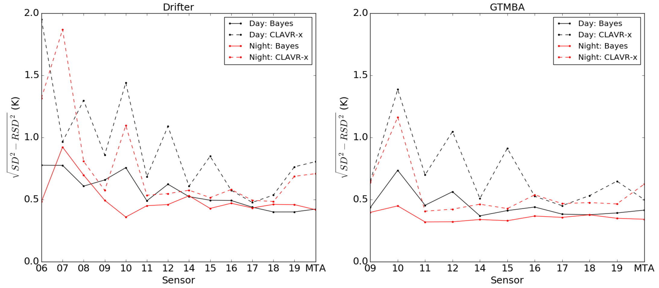
Figure 5 shows the $\sqrt{S{D}^2-RS{D}^2}$ metric for each sensor as a measure of uncertainty arising from outliers, for comparisons against drifting buoy and GTMBA data. For each in situ type, the day and nighttime statistics using each cloud mask are plotted. We see here that the metric for uncertainty arising from outliers is typically smaller when using the Bayesian algorithm, indicative of fewer cloud contaminated pixels which would increase the standard deviation. The uncertainty is also fairly consistent day and night, and throughout the sensor record. This is important in ensuring stability in the classification for the production of an SST climate data record. Uncertainties due to outliers are typically larger and more variable when cloud screening with CLAVR-x, particularly for the earlier sensors. The best performance for CLAVR-x is seen for NOAA-16, 17 and 18 during the day, where the metric is similar to that obtained when using the Bayesian algorithm. Overall, the uncertainty is smaller when comparing to GTMBA data than drifting buoys. This would be expected for two reasons: firstly, the GTMBA measurements are more accurate than those from drifting buoys as these instruments are calibrated. Secondly, GTMBA measurements are all made in the tropics under similar regimes, while the drifting buoy observations have a more global distribution. Although there may be a systematic bias in comparisons, these two factors would likely reduce the noise, thus reducing the standard deviation.

Despite the reduction in uncertainties due to outliers when using the Bayesian algorithm, the cold tail in the distribution of SST differences (largely responsible for the difference in the SD and RSD) is still more significant than in the ideal case. Cloud detection is performed after the radiance averaging in the GAC data production, and one possibility is that some cloudy pixels at the full resolution remain undetected following this averaging process. More generally, use of the textural PDF in the Bayesian masks aids the detection of cloud edges but may limit performance in regions of large SST gradients, for example across ocean fronts. The cloud detection methodology also has limited sensitivity to thin cirrus, but this is not critical for SST retrieval purposes.

We compare the absolute difference between the mean and median bias for each cloud mask with reference to drifting buoy data (

Table 10. Absolute difference between mean and median bias for two-channel (10.8 and 12 $\mathsf{\mu }$m) daytime and three-channel (3.7, 10.8 and 12 $\mathsf{\mu }$m) nighttime SST retrieval statistics using Bayesian and CLAVR-x cloud masks compared against drifting buoy data.

Sensor	Daytime Mean-Med Diff		Nighttime Mean-Med Diff
	Bayes	CLAVR-x	Bayes	CLAVR-x
NOAA-06 ${}^{*}$	0.017	0.155	0.068	0.059
NOAA-07	0.076	0.067	0.005	0.157
NOAA-08 ${}^{*}$	0.002	0.127	0.178	0.146
NOAA-09	0.038	0.045	0.06	0.068
NOAA-10 ${}^{*}$	0.006	0.123	0.021	0.071
NOAA-11	0.041	0.008	0.06	0.057
NOAA-12	0.05	0.155	0.049	0.052
NOAA-14	0.031	0.062	0.085	0.082
NOAA-15	0.044	0.107	0.072	0.083
NOAA-16	0.008	0.032	0.1	0.117
NOAA-17	0.025	0.024	0.088	0.1
NOAA-18	0.027	0.077	0.108	0.09
NOAA-19	0.049	0.166	0.127	0.167
MetOp-A	0.023	0.083	0.107	0.15

${}^{*}$ For these sensors the 12 $\mathsf{\mu }$m channel is not used in the retrieval as it is not present for AVHRR-1 sensors.

). As the mean will be affected by outliers, a larger difference provides some indication of the effect of undetected cloud on the SST retrieval. For each sensor, the cloudmask with the smallest mean-median difference is highlighted in bold. During the day, for the Bayesian mask, the largest mean-median difference for any sensor is 0.07 K indicating fewer cloud contaminated pixels overall than for CLAVR-x, where differences are as large as 0.17 K. The Bayesian mask shows the smallest differences for all sensors except NOAA-07, 11 and 17. At night the differences tend to be larger as cloud detection is more difficult without the additional information available from the visible channels. The maximum difference is seen for NOAA-19: 0.13 K when using the Bayesian mask and 0.17 K for CLAVR-x.

Table 11. Median bias, and absolute difference between mean and median bias for two-channel (10.8 and 12 $\mathsf{\mu }$m) daytime and three-channel (3.7, 10.8 and 12 $\mathsf{\mu }$m) nighttime SST retrieval statistics using Bayesian and CLAVR-x cloud masks compared against GTMBA data.

Sensor	Daytime Mean-Med Diff		Nighttime Mean-Med Diff
	Bayes	CLAVR-x	Bayes	CLAVR-x
NOAA-09	0.11	0.041	0.044	0.126
NOAA-10 ${}^{*}$	0.004	0.125	0.131	0.055
NOAA-11	0.099	0.006	0.101	0.13
NOAA-12	0.028	0.179	0.072	0.108
NOAA-14	0.014	0.07	0.103	0.143
NOAA-15	0.026	0.147	0.085	0.113
NOAA-16	0.011	0.025	0.133	0.18
NOAA-17	0.001	0.018	0.131	0.163
NOAA-18	0.004	0.064	0.148	0.159
NOAA-19	0.01	0.12	0.132	0.154
MetOp-A	0.017	0.003	0.124	0.169

${}^{*}$ For this sensor the 12 $\mathsf{\mu }$m channel is not used in the retrieval as it is not present for AVHRR-1 sensors.

shows the equivalent results using comparisons agains GTMBA arrays. The mean-median differences are small using the Bayesian mask for the majority of sensors, with values typically ≤ 0.02 K with the exception of NOAA-09 and NOAA-11. For CLAVR-x, differences exceed 0.1 K for NOAA-10, 12, 15 and 19. As with the comparison against drifiting buoys, the mean-median differences are larger at night, typically in the order of 0.1 K, but smaller using the Bayesian mask for all sensors apart from NOAA-10.

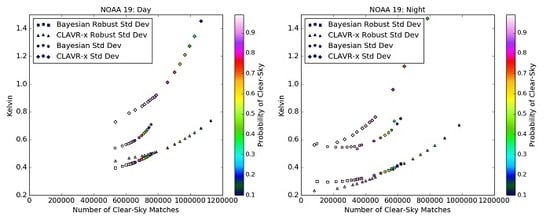
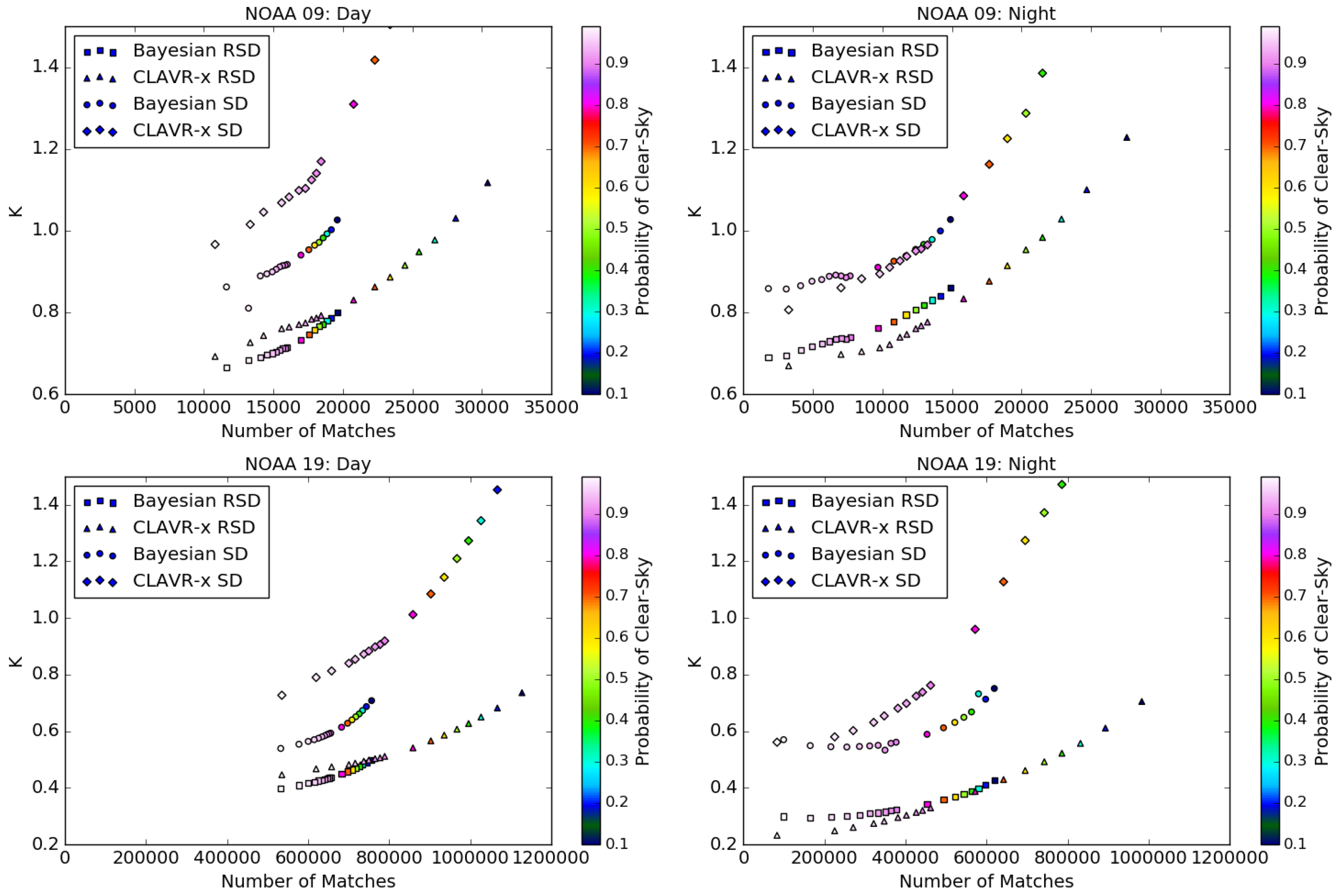
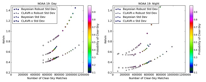
In Figure 6 we compare the SD and RSD for the two cloud detection algorithms using comparisons against drifting buoys as a function of the number of clear-sky matches. We threshold the Bayesian and CLAVR-x clear-sky probabilities at intervals of 0.1 between 0–0.9, and intervals of 0.01 for probabilities between 0.9–1. We present results for NOAA-09 in the upper panels and NOAA-19 in the lower panels in order to compare an early and late sensor in the data record. Daytime retrievals are shown on the left and nighttime retrievals on the right.

We find for all retrievals, for the probability intervals plotted, that the CLAVR-x mask gives a much wider range in the number of clear-sky matches. This is because the Bayesian probability of clear-sky is generally much more bimodal than CLAVR-x, with the majority of pixels classified as very likely to be clear-sky (≥0.9), or very likely to be cloud (≤0.1). The CLAVR-x probability distribution includes significantly more pixels classified between 0.1–0.9, where the appropriate clear/cloud classification is less obvious. The points indicating probability thresholds of 0.1–0.9 are therefore more tightly grouped for the Bayesian mask.

For NOAA-09 and clear-sky probability thresholds above 0.9 during the day, the Bayesian RSD typically ranges between 0.67–0.71 K, with CLAVR-x RSD’s between 0.69–0.78 K, also giving larger numbers of matches. At nighttime the RSD values are similar, with CLAVR-x giving comparable RSD values to the Bayesian mask for probabilities between 0.95–0.99, but with significantly more matches. The overall number of matches is fewer at night using both masks than during the day. We find that the Bayesian algorithm typically reduces the SD by ~0.1 K during the day, with only moderate data losses at probabilities ≥0.9. At night, the standard deviations for the two algorithms follow a similar curve for total matches exceeding 12,500, but below this the CLAVR-x algorithm gives a lower SD than the Bayesian for a given number of matches.

A similar result is seen for NOAA-19 although the overall number of matches is significantly larger both due to the lifetime of the instrument and the increased number of in situ observations. The RSDs are lower overall, typically between 0.4–0.51 K during the day and 0.23–0.32 K at night. During the day, the Bayesian mask gives lower RSD values than CLAVR-x, and also at night for the probability threshold of 0.9. For probabilities ≥ 0.93, and for total matches fewer than five hundred thousand, the CLAVR-x outperforms the Bayesian mask at night. During the day, the Bayesian algorithm significantly reduces the SD, by a factor of ~0.2 K for any given number of matches. At night, the standard deviations are lower for numbers of matches greater than two hundred thousand. The percentage reduction in the number of matches for a given probability at night is lower for NOAA-19 than NOAA-09. At a probability threshold of 0.9 we see a ~45% for NOAA-09 and ~15% for NOAA-19.

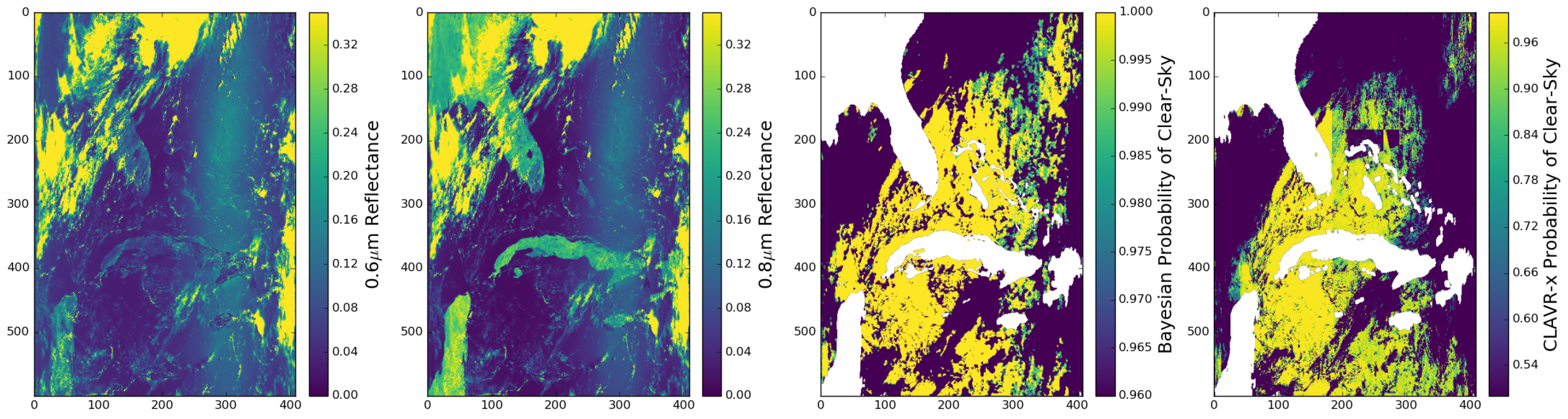
One region in which cloud detection is particularly challenging during the day is in the presence of sunglint. An example image from MetOp-A is shown in Figure 7, displaying the 0.6 and 0.8 $\mathsf{\mu }$m reflectance in the left hand plots. The sunglint features can be seen on the right of these images as a band running vertically, most prominent in the top half of the image. Sunglint increases the brightness of the ocean surface, and where reflectance features are used to detect cloud, sunglint areas are typically partially or completely flagged as cloud. The plots on the right hand side of Figure 7 show the Bayesian and CLAVR-x probabilities of clear-sky over the same region. Note these are provided on different scales for each mask. We see that the CLAVR-x mask performs poorly in the sunglint region with clear-sky probabilities falling below 0.5 across some of the region. There is evidence of problems using some of the cloudy features in the CLAVR-x classifier here, as indicated by hard lines in the probability field in this region. Conversely, the Bayesian algorithm performs well. The colour scale used here is for clear-sky probabilities between 0.96–1.0. For most of the clear-sky regions in the image the probability exceeds 0.99, and we see only a very slight decrease in confidence to ~0.98 in sunglint affected areas, without the loss of structure as seen in the CLAVR-x mask. Typically, we threshold the probability of clear-sky at 0.9 over the ocean to produce a binary clear/cloud mask, so this woud not result in a loss of clear-sky data.

5. Conclusions

We present here a Bayesian cloud detection scheme applied to the AVHRR data record from NOAA-06 through to MetOp-A. There are two novel concepts in the application of this scheme to AVHRR, beyond those published previously [5]: (1) Application of empirical cloudy look-up tables from a single sensor to the entire data record without the need to generate sensor specific auxiliary data files; (2) Use of the visible channel simulation from RTTOV v11.3 in daytime cloud detection. We compare the algorithm performance against the operational CLAVR-x cloud detection scheme, using matches with in situ data from drifting buoys and the GTMBA array. We find that the Bayesian cloud detection consistently reduces the uncertainty due to outliers indicative of removing undetected cloud from the distribution. For most sensors, using the Bayesian cloud detection scheme also reduces the robust standard deviation, most notably for daytime SST retrievals. At night, we find comparable RSD values for the Bayesian and CLAVR-x algorithms, but CLAVR-x gives significantly more matches. We present a case study over a sunglint region, highlighting the use of visible channel simulations for daytime cloud detection. Identification of clear-sky in sunglint is typically challenging for cloud detection schemes, but we find that the Bayesian scheme shows only small reductions in clear-sky probabilities. The Bayesian cloud detection performance is reasonably consistent across the data record, despite calibration issues affecting particularly earlier sensors in the data record, and differences in channel availability for AVHRR-1, 2 and 3 instruments for SST retrieval. We find that the Bayesian algorithm compares favourably against the well-established CLAVR-x operational cloud masking algorithm.

References

1. Carbajal Henken, C.K.; Linstrot, R.; Preusker, R.; Fischer, J. FAME-C: Cloud property retrieval using synergistic AATSR and MERIS observations. Atmos. Meas. Tech. 2014, 7, 3873–3890. [Google Scholar] [CrossRef]
2. Stengel, M.; Mieruch, S.; Jerg, M.; Karlson, K.-G.; Scheirer, R.; Maddux, B.; Meirink, J.F.; Poulsen, C.; Siddans, R.; Walther, A.; et al. The Clouds Climate Change Initiative: Assessment of state-of-the-art cloud property retrieval schemes applied to AVHRR heritage measurements. Remote Sens. Environ. 2015, 162, 363–379. [Google Scholar] [CrossRef]
3. Bulgin, C.E.; Sembhi, H.; Ghent, D.; Remedios, J.J.; Merchant, C.J. Cloud clearing techniques over land for land surface temperature retrieval from the Advanced Along Track Scanning Radiometer. Int. J. Remote Sens. 2014, 35, 3594–3615. [Google Scholar] [CrossRef]
4. Friedl, M.A.; McIver, D.K.; Hodges, J.C.F.; Zhang, X.Y.; Muchoney, D.; Strahler, A.H.; Woodcock, C.E.; Gopal, S.; Schneider, A.; Cooper, A.; et al. Global land cover mapping from MODIS: Algorithms and early results. Remote Sens. Environ. 2002, 83, 287–302. [Google Scholar] [CrossRef]
5. Merchant, C.J.; Harris, A.R.; Maturi, E.; MacCallum, S. Probabilistic physically-based cloud screening of satellite infra-red imagery for operational sea surface temperature retrieval. Q. J. R. Meteorol. Soc. 2005, 131, 2735–2755. [Google Scholar] [CrossRef] [Green Version]
6. Műller, D.; Krasemann, H.; Brewin, R.J.W.; Brockmann, C.; Deschamps, P.-Y.; Doerffer, R.; Fomferra, N.; Franz, B.A.; Grant, M.G.; Groom, S.B.; et al. The Ocean Colour Climate Change Initiative: II. Spatial and temporal homogeneity of satellite data retrieval due to systematic effects in atmospheric correction processors. Remote Sens. Environ. 2015, 162, 257–270. [Google Scholar] [CrossRef]
7. Frey, R.A.; Ackerman, S.A.; Liu, Y.; Strabala, K.I.; Zhang, H.; Key, J.R.; Wang, X. Cloud Detection with MODIS. Part I: Improvements in the MODIS Cloud Mask for Collection 5. J. Atmos. Ocean. Technol. 2008, 25, 1057–1072. [Google Scholar] [CrossRef]
8. Rossow, W.B.; Garder, L.C. Cloud Detection Using Satellite Measurements of Infrared and Visible Radiances for ISCCP. J. Clim. 1993, 12, 2341–2369. [Google Scholar] [CrossRef]
9. Závody, A.M.; Mutlow, C.T.; Llewellyn-Jones, D.T. Cloud Clearing over the Ocean in the Processing of Data from the Along-Track Scanning Radiometer (ATSR). J. Atmos. Ocean. Technol. 2000, 17, 595–615. [Google Scholar] [CrossRef]
10. Baum, B.A.; Tovinkere, V.; Titlow, J.; Welch, R.M. Automated Cloud Classification of Global AVHRR Data Using a Fuzzy Logic Approach. J. Appl. Meteorol. 1997, 36, 1519–1540. [Google Scholar] [CrossRef]
11. Gomez-Chova, L.; Munoz-Mari, J.; Amoros-Lopez, J.; Izquierdo-Verdiguier, E.; Camps-Valls, G. Advances in synergy of AATSR-MERIS sensors for cloud detection. In Proceedings of the Geoscience and Remote Sensing Symposium, Melbourne, VIC, Australia, 21–26 July 2013; pp. 4391–4394. [Google Scholar]
12. Bulgin, C.E.; Eastwood, S.; Embury, O.; Merchant, C.J.; Donlon, C. Sea surface temperature climate change intiative: Alternative image classification algorithms for sea-ice affected oceans. Remote Sens. Environ. 2015, 162, 396–407. [Google Scholar] [CrossRef]
13. Heidinger, A.K.; Evan, A.T.; Foster, M.J.; Walther, A. A Naive Bayesian Cloud-Detection Scheme Derived from CALIPSO and Applied within PATMOS-x. J. Appl. Meteorol. Climatol. 2012, 51, 1129–1144. [Google Scholar] [CrossRef]
14. Islam, T.; Rico-Ramirez, M.A.; Srivastava, P.K.; Dai, Q.; Han, D.; Gupta, M.; Zhuo, L. CLOUDET: A Cloud Detection and Estimation Algorithm for Passive Microwave Imagers and Sounders Aided by Naive Bayes Classifier and Multilayer Perceptron. IEEE J. Sel. Top. Appl. Earth Obs. Remote Sens. 2015, 8, 4296–4301. [Google Scholar] [CrossRef]
15. Merchant, C.J.; Embury, O.; Roberts-Jones, J.; Fiedler, E.; Bulgin, C.E.; Corlett, G.K.; Good, S.; McLaren, A.; Rayner, N.; Morak-Bozzo, S.; et al. Sea surface temperature datasets for climate applications from Phase 1 of the European Space Agency Climate Change Initiative (SST CCI). Geosci. Data J. 2014, 1, 179–191. [Google Scholar] [CrossRef]
16. Embury, O.; Merchant, C.J. A reprocessing for climate of sea surface temperature from the Along-Track Scanning Radiometers: A new retrieval scheme. Remote Sens. Environ. 2012, 116, 47–61. [Google Scholar] [CrossRef]
17. Dee, D.P.; Uppala, S.M.; Simmons, A.J.; Berrisford, P.; Poli, P.; Kobayashi, S.; Andrae, U.; Balmaseda, M.A.; Balsamo, G.; Bauer, P.; et al. The ERA-Interim reanalysis: Configuration and performance of the data assimilation system. Q. J. R. Meterol. Soc. 2011, 137, 553–597. [Google Scholar] [CrossRef]
18. EUMETSAT. AVHRR Level 1b Product Guide; EUMETSAT: Darmstadt, Germany, 2011; EUM/OPS-EPS/MAN/04/0029, v3A. [Google Scholar]
19. Rao, C.R.N.; Chen, J. Post-launch calibration of the visible and near-infrared channels of the Advanced Very High Resolution Radiometer on the NOAA-14 spacecraft. Int. J. Remote Sens. 1996, 17, 2743–2747. [Google Scholar] [CrossRef]
20. Heidinger, A.K.; Straka, W.C., III; Molling, C.C.; Sullivan, J.T.; Wu, X. Deriving an inter-sensor consistent calibration for the AVHRR solar reflectance data record. Int. J. Remote Sens. 2010, 24, 6493–6517. [Google Scholar] [CrossRef]
21. Bhatt, R.; Doelling, D.R.; Scarino, B.R.; Gopalan, A.; Haney, C.O.; Minnis, P.; Bedka, K.M. A Consistent AVHRR Visible Calibration Record Based on Multiple Methods Applicable for the NOAA Degrading Orbits. Part 1: Methodology. J. Atmos. Ocean. Technlol. 2016, 33, 2499–2515. [Google Scholar] [CrossRef]
22. Vermote, E.; Kaufman, Y.J. Absolute calibration of AVHRR visible and near-infrared channels using ocean and cloud views. Int. J. Remote Sens. 1995, 16, 2317–2340. [Google Scholar] [CrossRef]
23. Walton, C.C.; Sullivan, J.T.; Rao, C.R.N.; Weinreb, M. Corrections for detector nonlinearities and calibration inconsistencies of the infrared channels of the Advanced Very High Resolution Radiometer. J. Geophys. Res. 1998, 103, 3323–3337. [Google Scholar] [CrossRef]
24. Mittaz, J.P.D.; Harris, A.R.; Sullivan, J.T. A Physical Method for the Calibration of the AVHRR-3 Thermal IR Channels 1: The Prelaunch Calibration Data. J. Atmos. Ocean. Technol. 2009, 26, 996–1019. [Google Scholar] [CrossRef]
25. Mittaz, J.P.D.; Harris, A.R. A Physical Method for the Calibration of the AVHRR/3 Thermal IR Channels. Part II: An In-Orbit Comparison of the AVHRR Longwave Thermal IR Channels on board MetOp-A with IASI. J. Atmos. Ocean. Technol. 2011, 28, 1072–1087. [Google Scholar] [CrossRef]
26. Wang, L.; Cao, C. On-Orbit Calibration Assessment of AVHRR Longwave Channels on MetOp-A Using IASI. IEEE Trans. Geosci. Remote Sens. 2008, 46, 4005–4013. [Google Scholar] [CrossRef]
27. Mittaz, J.P.D.; Bali, M.; Harris, A.R. The calibration of broad band infrared sensors: Time variable biases and other issues. In Proceedings of the EUMETSAT Meteorological Satellite Conference, Vienna, Austria, 16–20 September 2013. [Google Scholar]
28. Wang, L.; Goldberg, M.; Wu, X.; Cao, C.; Iacovazzi, R.A., Jr.; Yu, F.; Li, Y. Consistency assessment of Atmsopheric Infrared Sounder and Infrared Atmospheric Sounding Interferometer radiances: Double differences verses simultaneous nadir overpasses. J. Geophys. Res. 2011, 116. [Google Scholar] [CrossRef]
29. Hocking, J.; Rayer, P.; Rundle, D.; Saunders, R.; Matricardi, M.; Geer, A.; Brunel, P.; Vidot, J. RTTOV v11 Users Guide; NWP SAF: Exeter, UK NWOSAF-MO-UD-028. Available online: www.nwpsaf.eu/site/download/documentation/rtm/docs_rttov11/users_guide_11_v1.4.pdf?b188a8&b188a8 (accessed 8 January 2018).
30. Cox, C.E.; Munk, W. Measurements of the roughness of the sea surface form the sun’s glitter. J. Opt. Soc. Am. 1954, 44, 838–850. [Google Scholar] [CrossRef]
31. Block, T.; Embacher, S.; Merchant, C.J.; Donlon, C. High performance software framework for the calculation of satellite-to-satellite data matchups (MMS version 1.2). Geosci. Model Dev. Discuss. 2017. [Google Scholar] [CrossRef]
32. National Snow and Ice Data Centre, Climatological Monthly Maximum Sea Ice Extent Dataset. Available online: www.nsidc.org/data/pm/ocean-masks (accessed 22 November 2017).
33. Karlsson, K.-G.; Anttila, K.; Trentmann, J.; Stengel, M.; Meirink, J.F.; Devasthale, A.; Hanschmann, T.; Kothe, S.; Jääkeläinen, E.; Sedlar, J.; et al. CLARA-A2: CM SAF Cloud, Albedo and surface RAdiation dataset from AVHRR data—Edition 2. Satell. Appl. Facil. Clim. Monit. 2017. Available online: https://doi.org/10.5676/EUM_SAF_CM/CLARA_AVHRR/V002 (accessed 8 January 2018).
34. Tonboe, R.T.; Eastwood, S.; Lavergne, T.; Sorensen, A.M.; Rathmann, N.; Dybkjaer, G.; Pedersen, L.T.; Hoyer, J.L.; Kern, S. The EUMETSAT sea ice concentration climate data record. Cryosphere 2016, 10, 2275–2290. [Google Scholar] [CrossRef]
35. Chevalier, F. Sampled Database of 60-Level Atmospheric Profiles from ECMWF Analyses; NWP SAF Report 4; ECMWF: Reading, UK, 2002; Available online: http://www.emwf.int/publications/library/do/references/show?id=83287 (accessed 8 January 2018).
36. Uppala, S.; Kalberg, P.W.; Simmons, A.J. The ERA-40 reanalysis. Q. J. R. Meteorol. Soc. 2005, 131, 2961–3012. [Google Scholar] [CrossRef]
37. Merchant, C.J.; Le Borgne, P.; Marsouin, A.; Roquet, H. Optimal estimation of sea surface temperature from split-window observations. Remote Sens. Environ. 2008, 112, 2469–2484. [Google Scholar] [CrossRef]
38. National Oceanic and Atmospheric Adminstration. Global Tropical Moored Buoy Array, Pacific Marine Environmental Laboratory. Available online: www.pmel.noaa.gov/gtmba/ (accessed 8 January 2018).
Figure 1. Daytime equator overpass times for AVHRR sensors as a function of instrument lifetime.
Remotesensing 10 00097 g001
Figure 2. Observed reflectance as a function of RTTOV v11.3 radiative transfer model (RTM) reflectance for Channel 1, 0.6 μ m (blue) and Channel 2, 0.8 μ m (red). Joined data points show data binned at 0.01 in the RTM reflectance with associated error bars. Solid lines show a linear regression of the observed reflectance against the RTM in each channel. Dashed black line shows the 1:1 relationship. Legend shows the gradient (Grad) and intercept (Int) of the linear fits to the data.
Remotesensing 10 00097 g002
Figure 3. Observed reflectance as a function of the corrected RTTOV v11.3 radiative transfer model (RTM) reflectance for Channel 1, 0.6 μ m (blue) and Channel 2, 0.8 μ m (red). The linear correction used is that defined in Figure 1. Joined data points show data binned at 0.01 in the RTM reflectance with associated error bars. Solid lines show a linear regression of the observed reflectance against the RTM in each channel. Dashed black line shows the 1:1 relationship. Legend shows the gradient (Grad) and intercept (Int) of the linear fits to the data.
Remotesensing 10 00097 g003
Figure 4. MetOp-A minus NOAA AVHRR brightness temperatures in the 3.7, 10.8 and 12 μ m channels plotted as a function of total column water vapour (TCWV) using RTTOV v11.3 simulations under clear-sky conditions. Results are binned in 1 kg m 2 TCWV, with joined points showing actual data for an atmospheric path length of 1. Solid lines show a cubic fit to these data and dashed lines show a cubic fit for the differences for each AVHRR simulated using an atmospheric path length of 1.8. Data are not shown for the atmospheric path length of 1.8 for clarity.
Remotesensing 10 00097 g004
Figure 5. S D 2 R S D 2 as a function of AVHRR sensor, as a measure of uncertainty arising from outliers. SST difference statistics are derived with reference to drifting buoys (left) and GTMBA data (right). Each plot shows day and nighttime retrieval statistics for the Bayesian and CLAVR-x cloud masks.
Remotesensing 10 00097 g005
Figure 6. Standard deviation (SD) and robust standard deviation (RSD) of the satellite minus in situ SST differences against drifting buoys for NOAA-09 (top) and NOAA-19 (bottom). Results are shown for daytime (left) and nighttime (right) retrievals. The SD and RSD values are plotted as a function of the number of matches and the probability of clear-sky. The clear-sky probability is denoted by the colour of each symbol, and the shape refers to the the mask (Bayesian, CLAVR-x) and the statistic (SD, RSD) as shown in the legend.
Remotesensing 10 00097 g006
Figure 7. Bayesian and CLAVR-x clear-sky probabilities in a sunglint affected region. Data are from MetOp-A on the 1st of August 2012. From left to right, plots show the 0.6 μ m reflectance, the 0.8 μ m reflectance, Bayesian clear-sky probabilty and CLAVR-x clear-sky probability. For the clear-sky probability plots, white areas denote land.
Remotesensing 10 00097 g007