Recursive Local Summation of RX Detection for Hyperspectral Image Using Sliding Windows

Abstract

Anomaly detection has received considerable interest for hyperspectral data exploitation due to its high spectral resolution. Fast processing and good detection performance are practically significant in real world problems. Aiming at these requirements, this paper develops a recursive local summation RX anomaly detection approach by virtue of sliding windows. This paper develops a recursive local summation RX anomaly detection approach by virtue of sliding windows. A causal sample covariance/correlation matrix is derived for local window background. As for the real-time sliding windows, the $Woodbury$ identity is used in recursive update equations, which could avoid the calculation of historical information and thus speed up the processing. Furthermore, a background suppression algorithm is also proposed in this paper, which removes the current under test pixel from the recursively update processing. Experiments are implemented on a real hyperspectral image. The experiment results demonstrate that the proposed anomaly detector outperforms the traditional real-time local background detector and has a significant speed-up effect on calculation time compared with the traditional detectors.

1. Introduction

Attributed to the high spectral resolution, hyperspectral images are now capable of uncovering many subtle signal sources that cannot be known by prior knowledge or be visually inspected by image analysts [1,2]. Signal sources appear as anomalies in the data, such as unexpected presence, low probability of occurrence, small sample population whose signature is spectrally distinct from spectral signatures of its surrounding data samples. As a result, anomaly detection has received considerable interest in hyperspectral imaging in the last twenty years [3,4,5,6].

The RX detector developed by Reed and Yu [3] is acknowledged to be the most widely used anomaly detector. The classic RX algorithm is based on the global sample covariance matrix K, and is referred to as K-RXD. Since then, many RX-like anomaly detectors have been proposed [7,8,9,10,11,12,13]. Of particular interest are RXD using global sample correlation matrix R (R-RXD) [7,8], and RXD based on local background covariance matrix (L-RXD) [9]. The L-RXD uses not only spectral information but also spatial information to bring benefit for detection performance [10]. However, it may fail to obtain the best detection performance due to the penuriousness and unicity of local background distribution in every local window. A local summation anomaly detection (LSAD) is proposed in [13] by combining multiple local neighboring distributions of the pixel under test to get better performance. LSAD can be considered as a local summation RXD (LS-RXD) using subspace feature projection for the stable local covariance estimation.

The hyperspectral remote sensing has developed rapidly in recent years, but as the satellite relocation cycle becomes shorter, some new problems come out. For instance, the massive data has brought some challenges to the data transmission and storage. Moreover, for the anomaly detection problem, the anomalies such as moving targets may show up for a short time and disappear quickly. In this case, timely detection is necessary. However, data transmission is quite time-consuming, to achieve timely detection, developing the recursive anomaly detection algorithms is important and necessary. Recently, several real-time anomaly detection methods [14,15,16,17,18,19] have been proposed. Specifically, real-time causal process of K-RXD and R-RXD detector (called as RT-CK-RXD, RT-CR-RXD) were developed in [14]. The real-time R-RXD and constrained energy minimization (CEM) are optimized and integrated in a dual-mode parallel Field-Programmable Gate Array (FPGA) based hardware platform in [16]. Unlike the RT-CR-RXD, in the FPGA-based implementations, each pixel under test is located in the middle region of the background, which can improve the performance of target detection. The computational performance of real-time causal linewise progressive anomaly detection (RCLPAD) based on Cholesky decomposition along with linear system solving were developed in [17]. An advanced anomaly detector using causal sliding array windows to capture local autocorrelation matrix statistics in the sense of causality was developed (CSA-RXD) [18], by virtue of causal sliding windows, a causal sample correlation matrix can be derived for causal anomaly detection. Recursive update equations are also derived and thus speed up real-time processing. A real-time L-RXD using the local casual square window is proposed in [19]. However, the method proposed in [19] still needs to calculate the inverse of a matrix to detect each pixel. Compared with sliding array window, setting a sliding square window usually contains much more spectral-spatial integration information. This paper addresses this issue and further develops the recursive processing for LS-RXD based on sliding square window. The contribution of this work is based on two points: a recursive version of LS-RXD according to a causal relation from the $Woodbury$ identity, which reduce the runtime; and a background suppression algorithm integrated with the recursive procedure, which improves the detection accuracy.

The rest of the paper is organized as follows. In Section 2, several related RX anomaly detectors are briefly covered. Section 3 provides the design of recursive sliding window detector. Section 4 demonstrates the experiments of the proposed algorithm compared with some traditional anomaly detection algorithms. Finally, Section 5 draws our conclusions.

2. Related Anomaly Detectors

In this section, we provide a short overview of K-RXD, L-RXD and LS-RXD.

Assume that ${\left\{{\mathit{r}}_i\right\}}_{i=1}^N$ is a set of data sample vectors, and ${\mathit{r}}_i={(r_{i1},r_{i2},..,r_{iL})}^T$ is the ith data sample vector, where L is the total number of spectral bands.

2.1. K-RXD

The K-RXD, denoted by ${\delta }_{K-RXD}\left(\mathit{r}\right)$, is specified as follows:

$${\delta }_{K-RXD}\left(\mathit{r}\right)={(\mathit{r}-\mathit{\mu })}^T{\mathit{K}}^{-1}(\mathit{r}-\mathit{\mu })$$

(1)

where $\mathit{\mu }=(1/N){\sum }_{i=1}^N{\mathit{r}}_i$ is the global sample mean and $\mathit{K}=(1/N){\sum }_{i=1}^N({\mathit{r}}_i-\mathit{\mu }){({\mathit{r}}_i-\mathit{\mu })}^T$ is the sample data covariance. The form of ${\delta }_{K-RXD}$ in (1) is actually the well know Mahalanobis distance between the data sample being detected and global sample mean. It should be pointed out that the model assumes the data arise from two normal probability density functions with the same covariance matrix but different means.

2.2. L-RXD

Local anomaly detection is very important since the global RX anomaly detector fails to work when the anomalies are relatively small or only distinct from the local surroundings, but buried in the global background. The most widely used local anomaly detection algorithm is derived from the commonly used RXD, named as local-RX detector (L-RXD). The L-RXD, denoted by ${\delta }_{L-RXD}\left(\mathit{r}\right)$, is specified by:

$${\delta }_{L-RXD}\left(\mathit{r}\right)={(\mathit{r}-{\mathit{\mu }}_{\mathit{W}})}^T{{\mathrm{\Sigma }}_{\mathit{W}}}^{-1}(\mathit{r}-{\mathit{\mu }}_{\mathit{W}})$$

(2)

where ${\mathit{\mu }}_{\mathit{W}}$ is the local sample mean of a square window of size $\omega \times \omega$ pixels, centered at pixel $\mathit{r}$ and ${\mathrm{\Sigma }}_{\mathit{W}}$ is the background data sample covariance matrix of the local window $\mathit{W}$.

For L-RXD, a window of the selected size should be chosen firstly. The window size should not be too large or too small to obtain considerable background estimation.

2.3. LS-RXD

The traditional L-RXD exploits only one sliding window to estimate the neighborhood background statistic for the pixel under test. It is difficult to detect a multi-pixels anomaly target by L-RXD if the local distributions of some windows are mostly occupied by anomaly pixels because the background statistic will be contaminated seriously by anomaly pixels. In order to solve this problem, a local summation RX detector is proposed in [13]. Figure 1 takes $3\times 3$ size multiple local windows to demonstrate the implementation of the local summation strategy.

As illustrated in Figure 1, nine local windows will be taken for the pixel under test, represented by a yellow pixel if the local window is chosen to be $3\times 3$ size. For an $\omega \times \omega$ size local window, the sliding filter contains $\omega \times \omega$ local windows for summation. The summation detector result for the pixel under test $\mathit{r}$ is specified by

$${\delta }_{LS-RXD}\left(\mathit{r}\right)=\sum _{i=1}^{\omega \times \omega }{(\mathit{r}-{\mathit{\mu }}_{{\mathit{W}}_{\mathit{i}}})}^T{{\mathrm{\Sigma }}_{{\mathit{W}}_i}}^{-1}(\mathit{r}-{\mathit{\mu }}_{{\mathit{W}}_{\mathit{i}}})$$

(3)

where ${\mathit{W}}_i$ is the local pixel samples dataset from window i, ${\mu }_{{\mathit{W}}_i}$ and ${\mathrm{\Sigma }}_{{\mathit{W}}_i}$ are the mean vector and covariance matrix of ${\mathit{W}}_i$, respectively.

Suppose that the pixel samples dataset in the local window is denoted as $\mathit{W}=\left\{{\mathit{r}}_{p_{ij}}\right\}$, where $i=1,2,..,\omega$, $j=1,2,..,\omega$ and $p_{ij}$ is the global location of ${\mathit{r}}_{p_{ij}}$ in the whole data set ${\left\{{\mathit{r}}_i\right\}}_{i=1}^N$. As a matter of fact, the LS-RXD specified by (3) can be implemented by recursively updating the detection result of each pixel in $\mathit{W}$ as the window is sliding, that is

$${\delta }_{LS-RXD}^{t+1}\left({\mathit{r}}_{p_{ij}}\right)={\delta }_{LS-RXD}^t\left({\mathit{r}}_{p_{ij}}\right)+{({\mathit{r}}_{p_{ij}}-{\mathit{\mu }}_{\mathit{W}})}^T{{\mathrm{\Sigma }}_{\mathit{W}}}^{-1}({\mathit{r}}_{p_{ij}}-{\mathit{\mu }}_{\mathit{W}})$$

(4)

where ${\mathit{\mu }}_{\mathit{W}}$ and ${\mathrm{\Sigma }}_{\mathit{W}}$ are the mean vector and covariance matrix of $\mathit{W}$, ${\delta }_{LS-RXD}^t$ and ${\delta }_{LS-RXD}^{t+1}$ are the t, $t+1$ times updated detection result, respectively.

In doing so, the only difference between L-RXD and LS-RXD is that as the local window is sliding; only the detection result of the centered pixel in the local window is calculated by L-RXD, while the detection results of all $\omega \times \omega$ pixels in the local window are updated by LS-RXD.

It is worth noting that the local summation RX detector in [13] is called as LSAD for short. Subspace feature projection is used in LSAD to approximately calculate the ${\mathrm{\Sigma }}_{{{\mathit{W}}_i}^{-1}}$ in Equation 3 to enable LSAD with robust background feature statistics. However, it is difficult to realize a timely process due to the subspace feature projection in practice. Band selection onboard before data transmission is feasible to avert the singularity of an inversed local covariance. Therefore, we only focus on the recursive process of L-RXD and LS-RXD in the following.

3. Recursive LS-RXD

In the aforementioned local summation detection algorithms, a new local covariance matrix inversion is repeatedly calculated as the local window slides. The key issue of the recursive process of L-RXD and LS-RXD is how to perform a recursive computation for every independent covariance matrix inversion.

In what follows, we describe how to calculate the covariance matrix inversion of a casual sliding array window recursively.

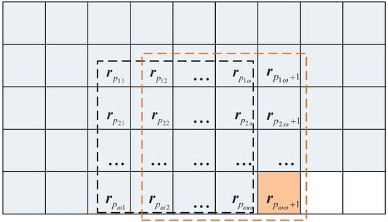
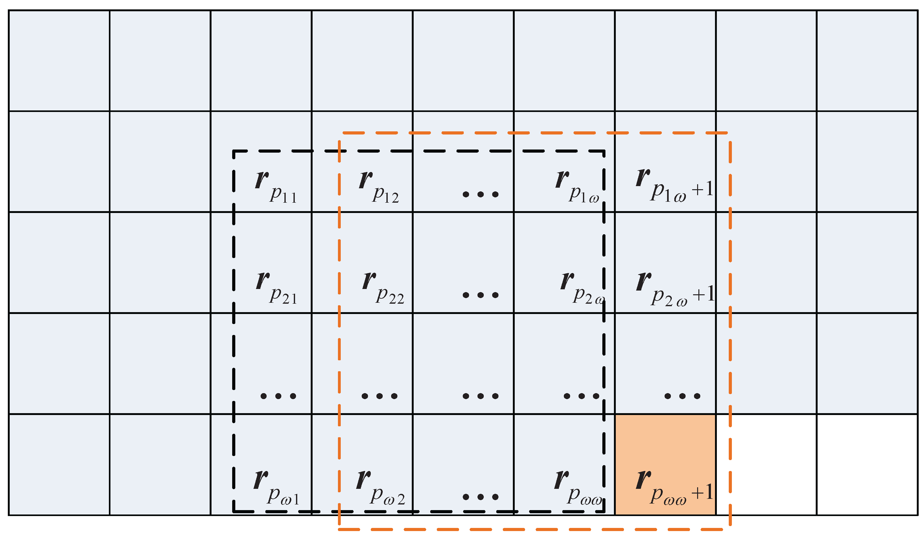
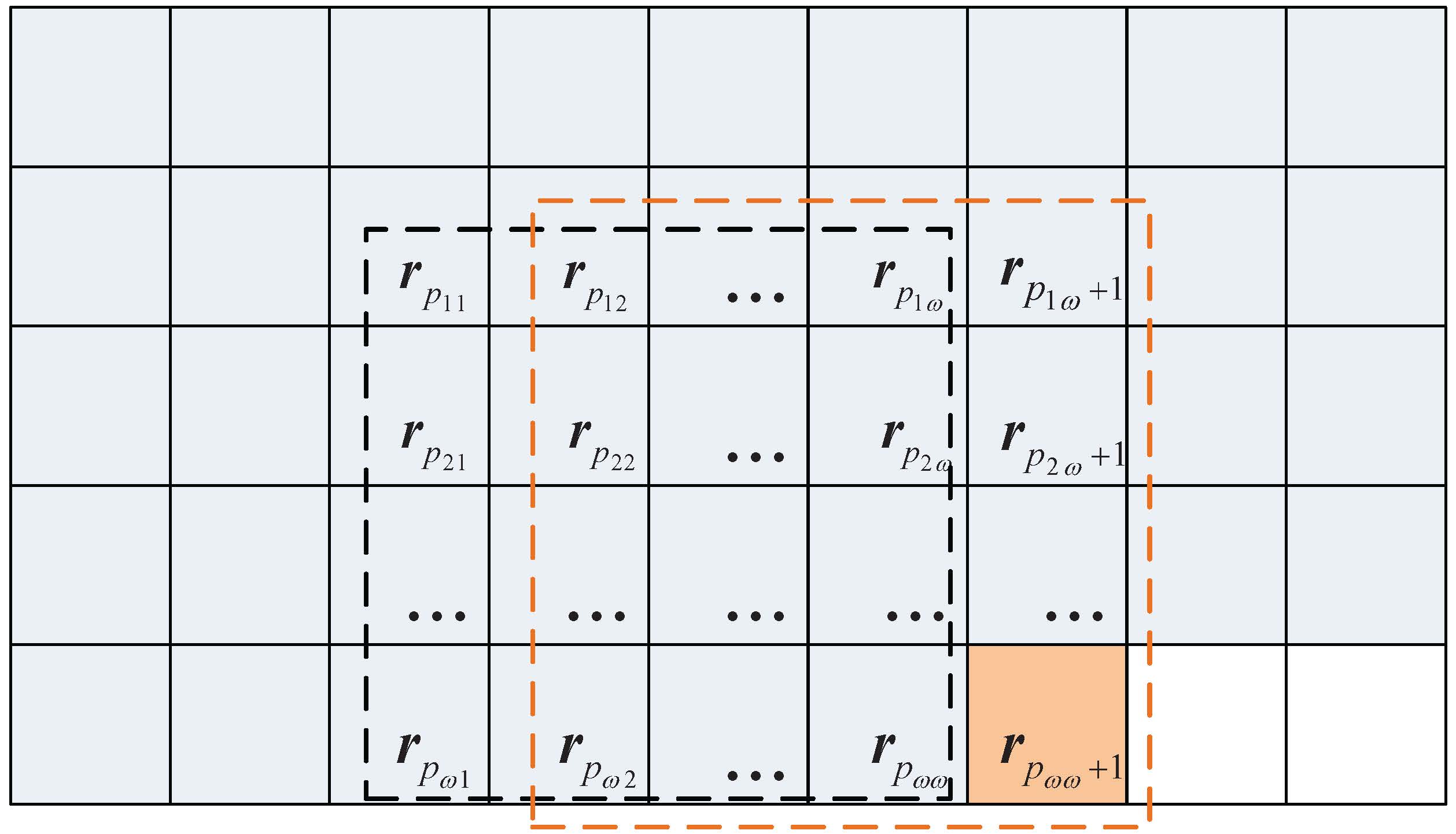
3.1. The Covariance Matrix Inversion of Causal Sliding Array Window

Figure 2 shows the causal sliding array window at ${\mathit{r}}_{n-1}$ depicted by dotted lines and the causal sliding array window at ${\mathit{r}}_n$ depicted by dashed lines, where a is the array window size. The farthest pixel ${\mathit{r}}_{n-a}$ from ${\mathit{r}}_n$ in the causal sliding array window at ${\mathit{r}}_n$ is removed from the causal sliding array window at ${\mathit{r}}_n$, while the most recent data sample vector ${\mathit{r}}_n$ is added to the causal sliding array window at ${\mathit{r}}_{n+1}$.

Defining ${\mathit{R}}_a\left(n\right)=(1/a){\sum }_{{\mathit{r}}_i\in \mathit{W}}{\mathit{r}}_i{\mathit{r}}_i^T$, where $\mathit{W}={\left\{{\mathit{r}}_i\right\}}_{i=n-a+1}^n$. ${\mathit{R}}_a\left(n\right)$ is called the “causal” sample auto correction matrix correlation matrix, and is formed by data sample vectors in the causal sliding array window. Then ${\mathit{R}}_a\left(n\right)$ can further be expressed as

$${\mathit{R}}_a\left(n\right)=[({\mathit{R}}_a(n-1)-\frac{{\mathit{r}}_{n-a}{\mathit{r}}_{n-a}^T}{a})+\frac{{\mathit{r}}_n{\mathit{r}}_n^T}{a}]$$

(5)

By repeatedly use of the following Woodbury matrix identity [20] twice:

$${[A+u{v}^T]}^{-1}=A^{-1}-\frac{\left[A^{-1}u\right]\left[v^T{A}^{-1}\right]}{1+v^T{A}^{-1}u}$$

(6)

the inverse of ${\mathit{R}}_a\left(n\right)$ can be updated recursively via ${\mathit{R}}_a^{-1}\left(n\right)$ by virtue of (7) and (8) [18]

$${\mathit{R}}_a^{-1}\left(n\right)={({\mathit{R}}_a(n-1)-\frac{{\mathit{r}}_{n-a}{\mathit{r}}_{n-a}^T}{a})}^{-1}-\frac{[{({\mathit{R}}_a(n-1)-\frac{{\mathit{r}}_{n-a}{\mathit{r}}_{n-a}^T}{a})}^{-1}\frac{{\mathit{r}}_n}{\sqrt{a}}][\frac{{\mathit{r}}_n^T}{\sqrt{a}}{({\mathit{R}}_a(n-1)-\frac{{\mathit{r}}_{n-a}{\mathit{r}}_{n-a}^T}{a})}^{-1}]}{1+\frac{{\mathit{r}}_n^T}{\sqrt{a}}{({\mathit{R}}_a(n-1)-\frac{{\mathit{r}}_{n-a}{\mathit{r}}_{n-a}^T}{a})}^{-1}\frac{{\mathit{r}}_n}{\sqrt{a}}}$$

(7)

$${({\mathit{R}}_a(n-1)-\frac{{\mathit{r}}_{n-a}{\mathit{r}}_{n-a}^T}{a})}^{-1}={{\mathit{R}}_a}^{-1}(n-1)+\frac{[{{\mathit{R}}_a}^{-1}(n-1)\frac{{\mathit{r}}_{n-a}}{\sqrt{a}}][\frac{{\mathit{r}}_{n-a}^T}{\sqrt{a}}{{\mathit{R}}_a}^{-1}(n-1)]}{1-\frac{{\mathit{r}}_{n-a}^T}{\sqrt{a}}{{\mathit{R}}_a}^{-1}(n-1)\frac{{\mathit{r}}_{n-a}}{\sqrt{a}}}$$

(8)

The “causal” covariance matrix formed by all the data sample vectors in the sliding array window can be specified by

$${\mathit{K}}_a\left(n\right)={\mathit{R}}_a\left(n\right)-{\mathit{\mu }}_a\left(n\right){\mathit{\mu }}_a^T\left(n\right)$$

(9)

where

$${\mathit{\mu }}_a\left(n\right)={\mathit{\mu }}_a(n-1)+(1/a)({\mathit{r}}_n-{\mathit{r}}_{n-a})$$

(10)

is the “causal” sample mean of sliding array window. Using $Woodbury$ matrix identity again, by letting $\mathit{A}={\mathit{R}}_a\left(n\right)$, $\mathit{u}=-{\mathit{\mu }}_a\left(n\right)$, $\mathit{v}={\mathit{\mu }}_a\left(n\right)$, then ${\mathit{K}}_a^{-1}\left(n\right)$ can be further expressed as

$${\mathit{K}}_a^{-1}\left(n\right)={\mathit{R}}_a^{-1}\left(n\right)+\frac{\left[{\mathit{R}}_a^{-1}\left(n\right){\mathit{\mu }}_a\left(n\right)\right]\left[{\mathit{\mu }}_a^T\left(n\right){\mathit{R}}_a^{-1}\left(n\right)\right]}{1-{\mathit{\mu }}_a^T\left(n\right){\mathit{R}}_a^{-1}\left(n\right){\mathit{\mu }}_a\left(n\right)}$$

(11)

By virtue of (7), (8), (10) and (11), ${\mathit{K}}_a^{-1}\left(n\right)$ can be updated recursively by ${\mathit{R}}_a^{-1}(n-1)$ and ${\mathit{\mu }}_a(n-1)$, via deleting the pixel ${\mathit{r}}_{n-a}$ and adding the current pixel ${\mathit{r}}_n$.

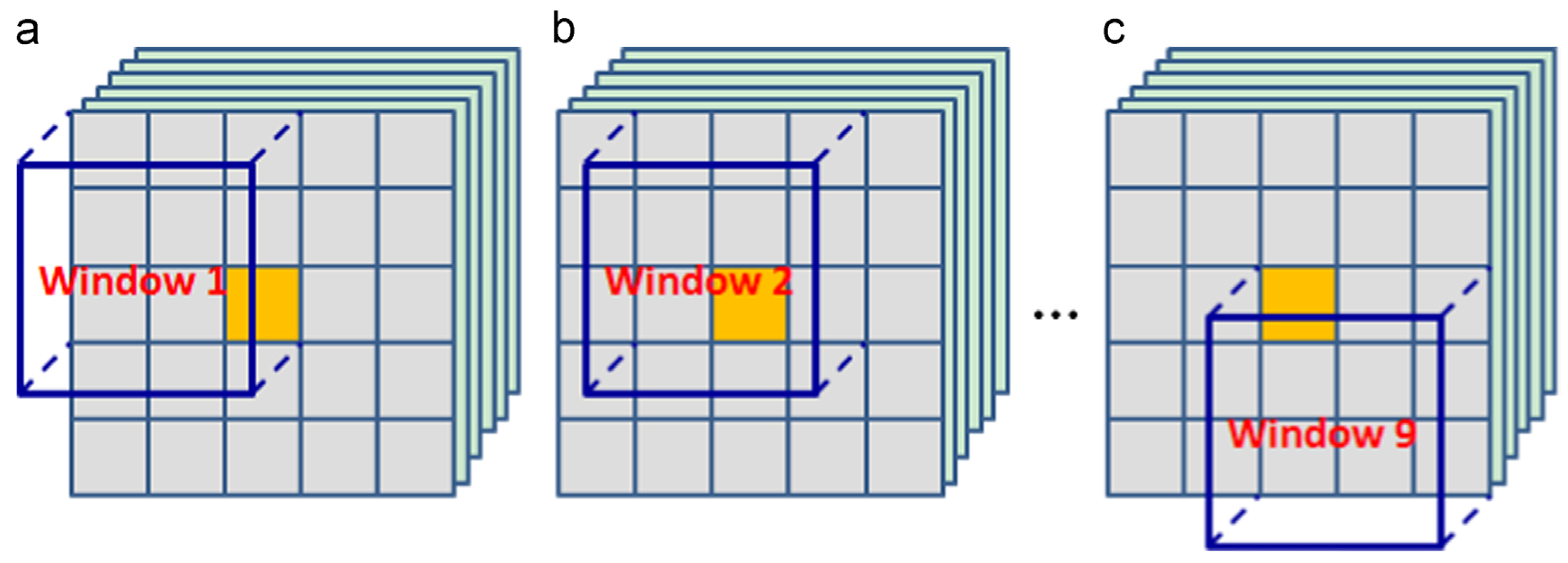
3.2. Recursive Processing of the Covariance Matrix Inversion of Sliding Window

Figure 3 illustrates two continually sliding windows with size of $\omega \times \omega$ depicted by black dashed lines and orange dashed lines, respectively, where ${\mathit{r}}_{p_{\omega \omega }+1}$ denotes the most recent received data sample vector. The sample data vectors update process in sliding windows can be implemented in $\omega$ steps by removing one pixel and adding one pixel each step. Suppose that $p_{\omega \omega }=n-1$, the inverses of correlation matrices of the local window at ${\mathit{r}}_{p_{\omega \omega }}$ and ${\mathit{r}}_{p_{\omega \omega }+1}$ are denoted as ${\mathit{R}}_{{\omega }^2}^{-1}(n-1)$ and ${\mathit{R}}_{{\omega }^2}^{-1}\left(n\right)$ respectively, and inverses of the covariance matrices of the local window at ${\mathit{r}}_{p_{\omega \omega }}$ and ${\mathit{r}}_{p_{\omega \omega }+1}$ are denoted as ${\mathit{K}}_{{\omega }^2}^{-1}(n-1)$ and ${\mathit{K}}_{{\omega }^2}^{-1}\left(n\right)$, respectively. In analogy with (7), (8), (10), and (11), ${\mathit{K}}_{{\omega }^2}^{-1}\left(n\right)$ can be updated recursively as follows.

For $i=1$ to $\omega$, do

$${({\mathit{R}}_{{\omega }^2}(n-1)-\frac{{\mathit{r}}_{p_{i1}}{\mathit{r}}_{p_{i1}}^T}{{\omega }^2})}^{-1}={\mathit{R}}_{{\omega }^2}^{-1}(n-1)+\frac{[{\mathit{R}}_{{\omega }^2}^{-1}(n-1)\frac{{\mathit{r}}_{p_{i1}}}{\omega }][\frac{{\mathit{r}}_{p_{i1}}^T}{\omega }{\mathit{R}}_{{\omega }^2}^{-1}(n-1)]}{1-\frac{{\mathit{r}}_{p_{i1}}^T}{\omega }{\mathit{R}}_{{\omega }^2}^{-1}(n-1)\frac{{\mathit{r}}_{p_{i1}}}{\omega }}$$

(12)

$${\mathit{R}}_{{\omega }^2}^{-1}\left(n\right)={({\mathit{R}}_{{\omega }^2}(n-1)-\frac{{\mathit{r}}_{p_{i1}}{\mathit{r}}_{p_{i1}}^T}{{\omega }^2})}^{-1}-\frac{[{({\mathit{R}}_{{\omega }^2}(n-1)-\frac{{\mathit{r}}_{p_{i1}}{\mathit{r}}_{p_{i1}}^T}{{\omega }^2})}^{-1}\frac{{\mathit{r}}_{p_{i\omega }}}{\omega }][\frac{{\mathit{r}}_{p_{i\omega }}^T}{\omega }{({\mathit{R}}_{{\omega }^2}(n-1)-\frac{{\mathit{r}}_{p_{i1}}{\mathit{r}}_{p_{i1}}^T}{{\omega }^2})}^{-1}]}{1+\frac{{\mathit{r}}_{p_{i\omega }}^T}{\omega }{({\mathit{R}}_{{\omega }^2}(n-1)-\frac{{\mathit{r}}_{p_{i1}}{\mathit{r}}_{p_{i1}}^T}{{\omega }^2})}^{-1}\frac{{\mathit{r}}_{p_{i\omega }}}{\omega }}$$

(13)

Meanwhile, update ${\mathit{R}}_{{\omega }^2}^{-1}(n-1)={\mathit{R}}_{{\omega }^2}^{-1}\left(n\right)$ after each iteration.

Then

$${\mathit{\mu }}_{{\omega }^2}^{-1}\left(n\right)={\mathit{\mu }}_{{\omega }^2}^{-1}(n-1)+(1/{\omega }^2)\left({\sum }_{i=1}^{\omega }({\mathit{r}}_{p_{i\omega }}-{\mathit{r}}_{p_{i1}})\right)$$

(14)

$${\mathit{K}}_{{\omega }^2}^{-1}\left(n\right)={\mathit{R}}_{{\omega }^2}^{-1}\left(n\right)+\frac{\left[{\mathit{R}}_{{\omega }^2}^{-1}\left(n\right){\mathit{\mu }}_{{\omega }^2}\left(n\right)\right]\left[{\mathit{\mu }}_{{\omega }^2}^T\left(n\right){\mathit{R}}_{{\omega }^2}^{-1}\left(n\right)\right]}{1-{\mathit{\mu }}_{{\omega }^2}^T\left(n\right){\mathit{R}}_{{\omega }^2}^{-1}\left(n\right){\mathit{\mu }}_{{\omega }^2}\left(n\right)}$$

(15)

3.3. Recursive Processing of LS-RXD

Except for the recursive processing of the covariance matrix inversion of the sliding window, some other issues should also be considered.

The first issue is the edge expansion. To ensure that there is no absence of detection on the edge of an image, the edge expansion is usually operated as a preprocessing for a local window detector. Due to the low probability of anomaly targets appearance in hyperspectral images, enplaned layers can be randomly chosen from the whole image [13]. With this consideration in mind, take the window with size of $3\times 3$ as an example. We design the sliding window strategy, depicted in Figure 4, where the yellow, blue and purple grids, respectively, denote the latest pixel received, the processed data and the pixels to be processed. As Figure 4 shows, when the sliding window meets the right board of the hyperspectral image, the next several sliding windows are across the border by moving down one line and adding new data one by one. The last sliding window moves to the right-bottom until the last sample data ${\mathit{r}}_{Row\times Col}$ is received. This design enables the recursive processing of LS-RXD more conveniently.

The second issue is how to keep track of which data sample vector should be removed and which data sample vector should be added as a matrix window moves on. Let $\mathit{W}={\left\{{\mathit{r}}_{p_{ij}}\right\}}_{i,j=1}^{\omega }$ denote the local sliding window in an image with size $Row\times Col$, where $p_{ij}$ is the global location of ${\mathit{r}}_{p_{ij}}$ in the whole data set ${\left\{{\mathit{r}}_i\right\}}_{i=1}^N$. For the first local window, $p_{ij}$ can be expressed as $p_{ij}=x_{(i-1)\times Col+j}$ . Using the strategy of Figure 4, it is very easy to update the global location of pixels in the follow-up window as $p_{ij}=p_{ij+1}$ successively.

After the aforementioned issues are solved, the recursive LS-RXD, called as R-LS-RXD can be obtained by

$${\delta }_{R-LS-RXD}\left({\mathit{r}}_{p_{ij}}\right)={\delta }_{R-LS-RXD}\left({\mathit{r}}_{p_{ij}}\right)+{({\mathit{r}}_{p_{ij}}-{\mathit{\mu }}_{{\omega }^2}\left(n\right))}^T{\mathit{K}}_{{\omega }^2}^{-1}\left(n\right)({\mathit{r}}_{p_{ij}}-{\mathit{\mu }}_{{\omega }^2}\left(n\right))$$

(16)

Three comments are worthwhile:

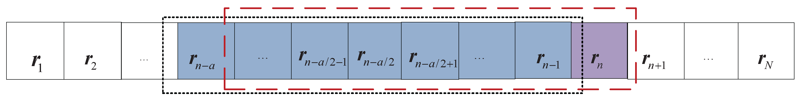
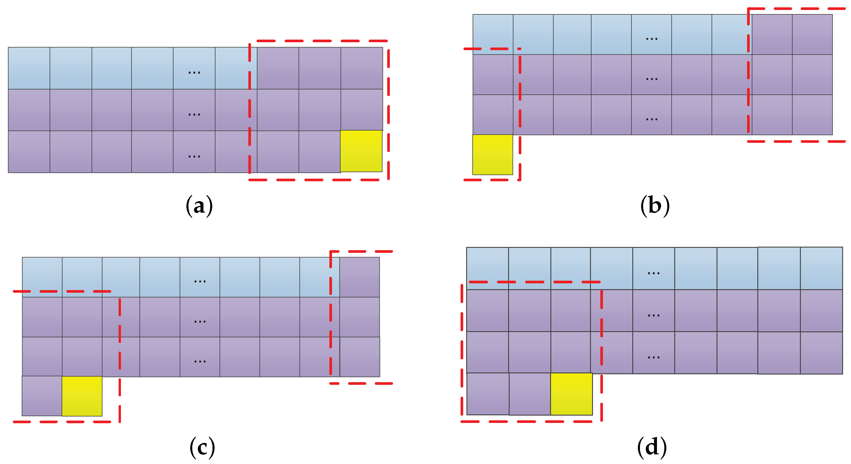
• It is important to note that, using the strategy of Figure 4, the updating counts of the detection value for the pixel located in several top and bottom lines of the image are less than $\omega$. This will result in the whole detection result being inconsistent. To solve this problem, the updating number of each pixel is counted, which is denoted as $N_{p_{ij}}$, and finally the detection result is obtained as ${\delta }_{R-LS-RXD}\left({\mathit{r}}_{p_{ij}}\right)/N_{p_{ij}}$
• To avoid the singularity problem of calculating the inverse of the sample correlation and covariance matrix used by anomaly detectors, $\omega \times \omega$ must at least equal to or greater than the total number of spectral bands [13,18].
• The whole design procedure is also suitable for recursive L-RXD which is not included here.

3.4. Background Suppression of Sliding Windows

This section mainly discusses the background suppression sliding window furthermore. It is not convenient to set the current under test pixel to conclude in the local window background with other data samples, because it will reduce the separation between background information and anomaly information separation while the current under test pixel is anomaly [21]. In order to suppress the background information and improve the detection performance, we need to remove the current under test pixel (${\mathit{r}}_k$) from the recursive update processing.

Assume that ${\mathit{R}}_k$ is the correlation matrix removed ${\mathit{r}}_k$, and ${\mathit{R}}_k$ is specified by

$$\begin{array}{cc}\hfill {\mathit{R}}_k& =\frac{1}{n-1}{\sum }_{i=1,i\ne k}^n{\mathit{r}}_i{\mathit{r}}_i^T=\frac{1}{n-1}({\sum }_{i=1}^n{\mathit{r}}_i{\mathit{r}}_i^T-{\mathit{r}}_k{\mathit{r}}_k^T)\hfill \\ \hfill & =\frac{n}{n-1}\frac{1}{n}{\sum }_{i=1}^n{\mathit{r}}_i{\mathit{r}}_i^T-\frac{1}{n-1}{\mathit{r}}_k{\mathit{r}}_k^T=\frac{n}{n-1}{\mathit{R}}_n-\frac{1}{n-1}{\mathit{r}}_k{\mathit{r}}_k^T\hfill \end{array}$$

(17)

Once using $Woodbury$ matrix identity, letting $A=\frac{n}{n-1}{\mathit{R}}_n$, $u=\frac{-1}{n-1}{\mathit{r}}_k$, $v={\mathit{r}}_k$, then

$$\begin{array}{cc}\hfill {\mathit{R}}_k^{-1}& ={(\frac{n}{n-1}{\mathit{R}}_n-\frac{1}{n-1}{\mathit{r}}_k{\mathit{r}}_k^T)}^{-1}\hfill \\ \hfill & =\frac{n-1}{n}{\mathit{R}}_n^{-1}+\frac{\left[\frac{n-1}{n}{\mathit{R}}_n^{-1}\frac{1}{n-1}{\mathit{r}}_k\right]\left[{\mathit{r}}_k^T\frac{n-1}{n}{\mathit{R}}_n^{-1}\right]}{1-{\mathit{r}}_k^T\frac{n-1}{n}{\mathit{R}}_n^{-1}\frac{1}{n-1}{\mathit{r}}_k}\hfill \end{array}$$

(18)

Assume that ${\mathit{\mu }}_k$ is the mean vector of background sample data removed ${\mathit{r}}_k$, the inverse of covariance matrix could be specified by

$${\mathit{K}}_{BS}^{-1}\left(n\right)={\mathit{R}}_k^{-1}\left(n\right)+\frac{\left[{\mathit{R}}_k^{-1}\left(n\right){\mathit{\mu }}_k\left(n\right)\right]\left[{\mathit{\mu }}_k^T\left(n\right){\mathit{R}}_k^{-1}\left(n\right)\right]}{1-{\mathit{\mu }}_k^T\left(n\right){\mathit{R}}_k^{-1}\left(n\right){\mathit{\mu }}_k\left(n\right)}$$

(19)

As a result, the background suppression recursive R-BS-LS-RXD can be specified by

$${\delta }_{R-BS-LS-RXD}\left({\mathit{r}}_k\right)={({\mathit{r}}_k-{\mathit{\mu }}_k\left(n\right))}^T{\mathit{K}}_{BS}^{-1}\left(n\right)({\mathit{r}}_k-{\mathit{\mu }}_k\left(n\right))$$

(20)

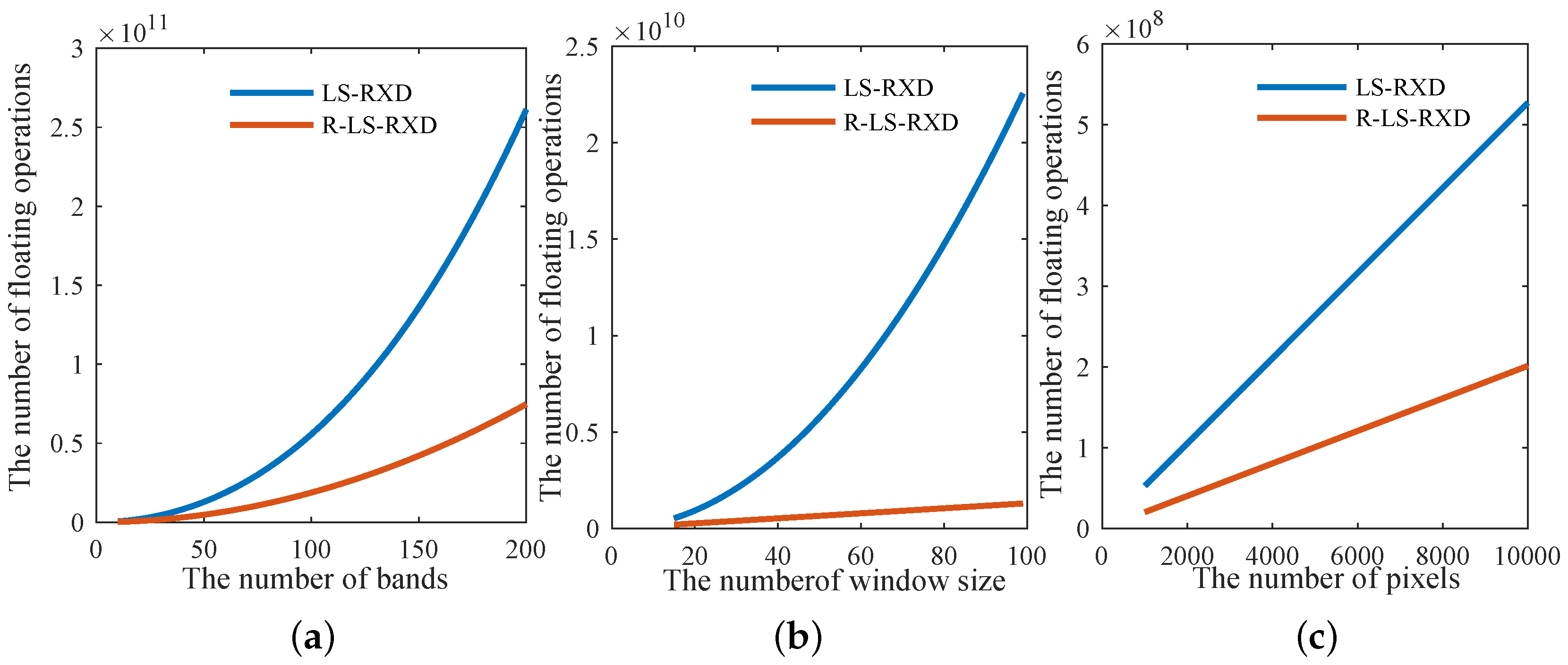
3.5. Computational Complexity Analysis

This section provides a detailed analysis on the computational complexity of calculating recursive update Equations (12)–(15).

The advantage of using causal sliding windows over local windows is the use of recursive Equations (12) and (13), where the $Woodbury$ identity is implemented twice, instead of recalculating each time as long as a new data sample vector comes in.

Table 1. Computation Complexity of Matrix Algebra.

Operation	Input	Output	Algorithm	Complexity
Matrix multiplication	Matrix a size $m\times n$; Matrix b size $n\times p$;	Matrix size $m\times p$	Schoolbook matrix multiplication	$O\left(mnp\right)$
Matrix inversion	Matrix size $m\times m$	Matrix size $m\times m$	Gauss-Jordan elimination Strassen algorithm Coppersmith-Winograd algorithm Williams algorithm	$O\left(n^3\right)$ $O\left(n^{2.807}\right)$ $O\left(n^{2.376}\right)$ $O\left(n^{2.373}\right)$

shows the computation complexity of matrix algebra. Based on the information in Table 1, the matrix inversion computation complexity is higher than the matrix multiplication computation.

The usage frequency of the $Woodbury$ matrix identity is determined by the size of the sliding window. Local background information is updated by calculating $\omega$ times of Equations (12) and (13), regardless of the number of pixels in the local background. Such a significant benefit arises from the recursive specialty in (12) and (13). Hence, the computational complexity of processing a single local window specified by its window size $\omega \times \omega$ requires $\omega$ times calculations of matrix multiplication. In addition, it only needs to calculate the inverse of the covariance matrix once.

Table 2. Computational Complexity for local summation RXD (LS-RXD) and recursive local summation RXD (R-LS-RXD).

Algorithm		LS-RXD			R-LS-RXD
Operator	Initialization	Input ${\mathit{r}}_{\mathit{n}}$			Input ${\mathit{r}}_{\mathit{n}}$
		${\mathit{\mu }}_{\mathit{a}}$	$\mathit{K}$	${\mathit{K}}^{\mathit{-}\mathit{1}}$	${\mathit{\mu }}_{\mathit{a}}$	$\mathbf{\text{Equation}}\mathbf{\left(}\mathbf{7}\mathbf{\right)}$	$\mathbf{\text{Equation}}\mathbf{\left(}\mathbf{8}\mathbf{\right)}$	${\mathit{K}}^{\mathbf{-}\mathbf{1}}$
flops	$L^3+2a(L^2+L)$	$(a+1)L$	$2a(L^2+L)$	$L^3$	$3L$	$\omega (6L^2+5L)$	$\omega (6L^2+5L)$	$6L^2+L$
sum		$N{L}^3+2aN{L}^2+3a(N+1)L$			$L^3+(2a+12N\omega +6N)L^2+(2a+4N+10N\omega )L$

tabulates the number of floating operations (flops) required for LS-RXD and R-LS-RXD, which update ${\mathit{K}}_a^{-1}\left(n\right)$ in different method, where the bands number is specified by L, local window size is specified by $a=\omega \times \omega$, and the pixels number to be processed is specified by N. These parameters determine the number of flops in the algorithm. Figure 5 plots the number of floating operations required for every algorithm versus L, a and N. The configurations of parameters are shown in

Table 3. Configuration of The Parameters.

Figure 5	Parameters
	$\mathit{L}$	$\mathit{\omega }$	$\mathit{N}$
(a)	10:5:200	15	10,000
(b)	10	15:2:99	10,000
(c)	10	15	1000:1000:10,000

.

As shown in Figure 5, the comparison of different anomaly detectors depends on the specific configuration of the parameters. Generally speaking, R-LS-RXD is faster than LS-RXD.

4. Results and Discussion

To demonstrate the performance of anomaly detection using recursive local summation RXD, two real hyperspectral image scenes were conducted for experiments. The first image data set is the Airborne Visible/Infrared Imaging Spectrometer (AVIRIS) image scene of Sandiego airport area which is located in California. A sub-image with size $100\times 100$ along with its ground truth are shown in Figure 6a,b, respectively. It was acquired through 224 spectral bands with a spectral coverage from 0.4 to 2.5 $\mathsf{\mu }\mathrm{m}$ where the spatial resolution is 3 m and spectral resolution is 20 nm. After removing low signal-to-noise ratio (SNR) and water absorption bands, a total of 126 spectral bands were used for experiments.

The second image data set is the Hyperspectral Digital Imagery Collection Experiment (HYDICE) image scene shown in Figure 7a which was collected in August 1995 from a flight altitude of 10,000 ft with the ground sampling distance approximately 1.56 m. This scene has been studied extensively by many reports such as [2,14]. It has a total of 169 bands which were used for the experiments with low signal/high noise bands: bands 1–3 and bands 202–210; and water vapor absorption bands: bands 101–112 and bands 137–153, removed. There are 15 panels with three different sizes of $3\mathrm{m}\times 3\mathrm{m}$, $2\mathrm{m}\times 2\mathrm{m}$ and $1\mathrm{m}\times 1\mathrm{m}$. Figure 7b shows the precise spatial locations of these 15 panels, where red pixels (R pixels) are the panel center pixels and the pixels in yellow (Y pixels) are panel boundary pixels mixed with the background (BKG) . As a result, there are a total of 19 R panel pixels. In particular, R panel pixels are denoted by $p_{ij}$ with rows indexed by $i=1,\cdots ,5$ and columns indexed by $j=1,2,3$ except that the panels in the 1st column with the 2nd , 3rd , 4th, 5th rows which are two-pixel panels, denoted by $p_{211}$, $p_{221}$, $p_{311}$, $p_{312}$, $p_{411}$, $p_{412}$, $p_{511}$, $p_{521}$. The 1.56 m-spatial resolution of the image scene suggests that most of the 15 panels are one pixel in size.

In order to quantitatively evaluate detection performance, receiver operating characteristic (ROC) curves are used to compare the different algorithms. Based on the provided ground truth, we can perform an analysis via ROC curves of the false alarm ratio ($Pf$) versus the detection ratio ($Pd$) by taking all the possible thresholds ($\tau$). We can further calculate the area under the ROC curve (AUC) for a quantitative performance analysis. The algorithm with a larger AUC value is regarded as a better performance.

Traditional ROC curves is a 2D plot represented by values of $Pf$ and $Pd$. Furthermore, we can plot another 2D ROC curve of $Pf$ and $\tau$, which provides crucial information of progressive background suppression as the threshold $\tau$ varies. when it comes to the interpretation of anomaly detection by visual inspection with no availability of ground truth or AUC values with similar performance.

Three experiments are conducted with the purpose of: (1) evaluating the influence of window size on the detection performance of R-LS-RXD; (2) comparing the detection performance of different algorithms; and (3) comparing computing times of different algorithms, respectively.

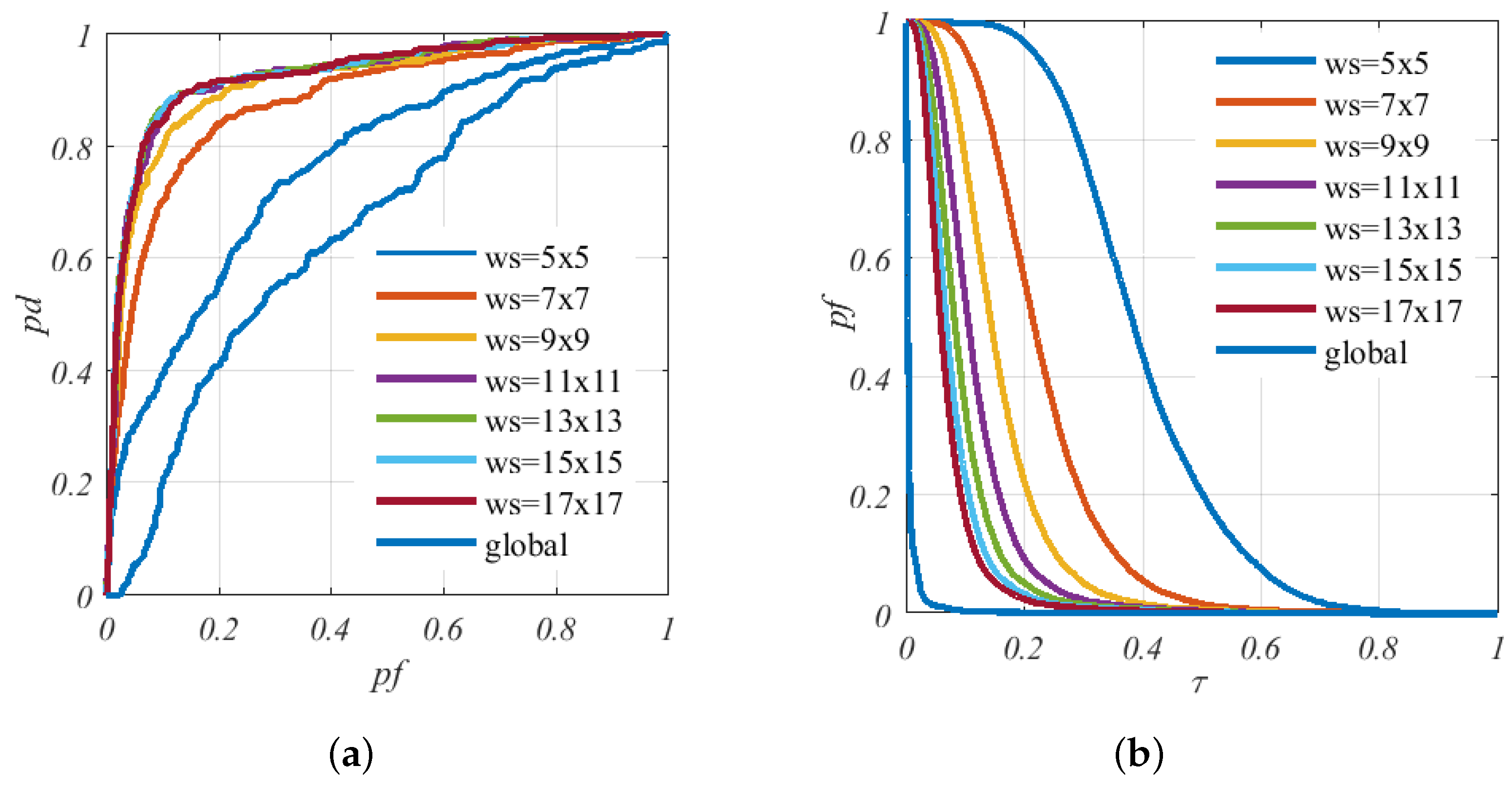
4.1. Optimum Size of Sliding Window

Band selection is very practical in anomaly detection [22,23]; nine bands are selected by signal-to-noise ratio estimation and maximal information (SNRE-MI) [23] in the experiment to obtain better result. To investigate the influence of window size on detection performance of R-LS-RXD, two hyperspectral images of different sensors (AVIRIS and HYDICE, respectively) in the previous section are used for experiments, the size of sliding window varies from $5\times 5$ up to $17\times 17$ with steps of two pixels side width. Figure 8a–g and Figure 9a–g show their detection abundance fractional maps with their detected abundance fractions in gray scale of AVIRIS and HYDICE hyperspectral image, respectively. According to the experiment, the detection result is poor with a window size of $5\times 5$, where the background and anomaly are difficult to separate for both sensors. Additionally, the performance begins to improve as the window size increases. When the window size is greater than or equal to $11\times 11$, detection performances are similar by visual inspection as shown in Figure 8 and Figure 9. Figure 8h and Figure 9h show the results of global background K-RXD detector for comparison.

In order for a further quantitative evaluation of detection performance with different window sizes, the ROC curves are implemented. To simplify our study, ROC curves for HYDICE data are not given, since the results are similar for both data sources. Figure 10 shows the ROC curves for AVIRIS data with different window sizes, with a traditional ($Pd$, $Pf$) ROC in (a) and a ($Pf$, $\tau$) curve analysis in (b), respectively. Additionally, the AUC values, denoted by $A_z$, are calculated for each ($Pd$, $Pf$) curves and ($Pf$, $\tau$) curves. In general, the higher the value of $A_z(Pd,Pf)$ and the lower the value of $A_z(Pf,\tau )$, the better the detection performance is. Results are tableted in

Table 4. Area under the ROC curve (AUC) values of ($Pd$, $Pf$) and ($Pf$, $\tau$) with different window sizes

Sensor	Window-Size	$\mathbf{5}\mathbf{\times }\mathbf{5}$	$\mathbf{7}\mathbf{\times }\mathbf{7}$	$\mathbf{9}\mathbf{\times }\mathbf{9}$	$\mathbf{11}\mathbf{\times }\mathbf{11}$	$\mathbf{13}\mathbf{\times }\mathbf{13}$	$\mathbf{15}\mathbf{\times }\mathbf{15}$	$\mathbf{17}\mathbf{\times }\mathbf{17}$	$\mathit{Global}$
AVIRIS	$A_z$($Pd$, $Pf$) $A_z$($Pf$, $\tau$)	0.7679 0.3461	0.8813 0.2059	0.9141 0.1389	0.9206 0.1086	0.9286 0.0873	0.9281 0.0752	0.9275 0.0648	0.6548 0.0080
HYDICE	$A_z$($Pd$, $Pf$) $A_z$ ($Pf$, $\tau$)	0.9895 0.2636	0.9973 0.1576	0.9985 0.1178	0.9988 0.0902	0.9988 0.0713	0.9986 0.0575	0.9982 0.0468	0.9878 0.0121

, with the best results highlighted.

Based on the result of Figure 10 and Table 4, as the window size goes up, the values of $A_z$ ($Pd$, $Pf$) are increased while the values of $A_z$ ($Pf$, $\tau$) are decreased. The detector reaches the best detection power in size $13\times 13$, and the best background suppression performs the best with size $17\times 17$. However, the trend of $A_z$ ($Pf$, $\tau$) decreasing obviously slows down when the window size increases from $13\times 13$ to $15\times 15$. When it comes to the global size background, the value of $A_z$ ($Pd$, $Pf$) decreases to an untrustworthy value and is difficult to be distinguished by visual inspection in Figure 8h and Figure 9h.

The conclusions for the experiment are as follows. As with the size of window increases, the sliding window RXD window RXD detector obtains better detection performances. However, $13\times 13$ is the optimum size for a Sandiego hyperspectral image. As an alternative interpretation, although a larger window size results in better background suppression, the detection performance is much more important in the detector evaluation.

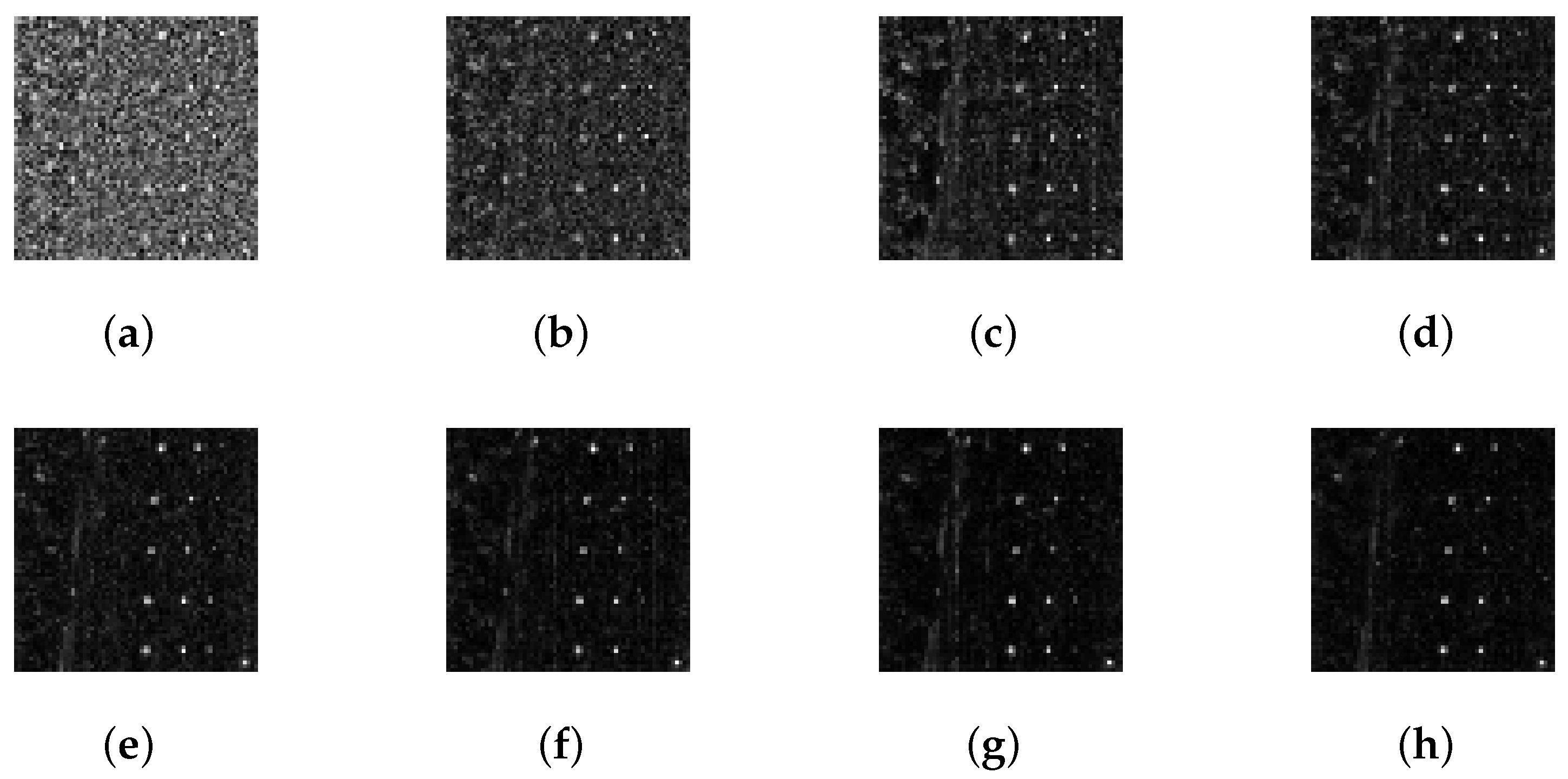
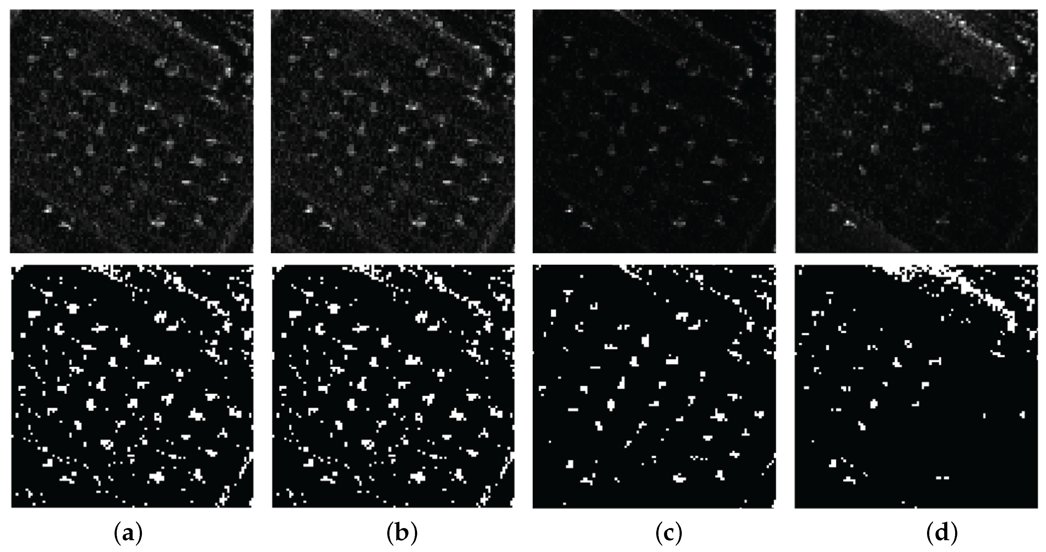
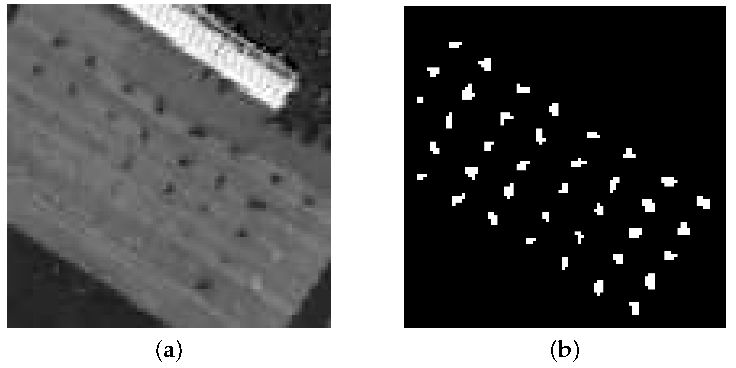
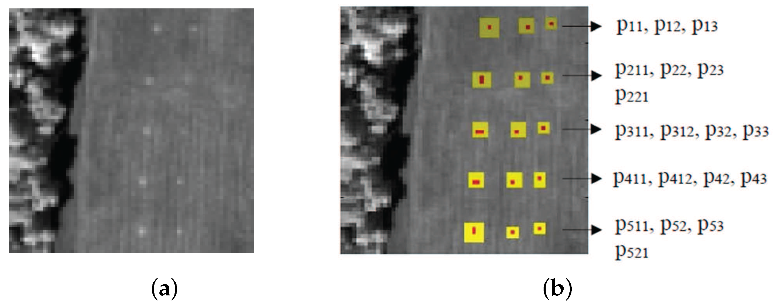
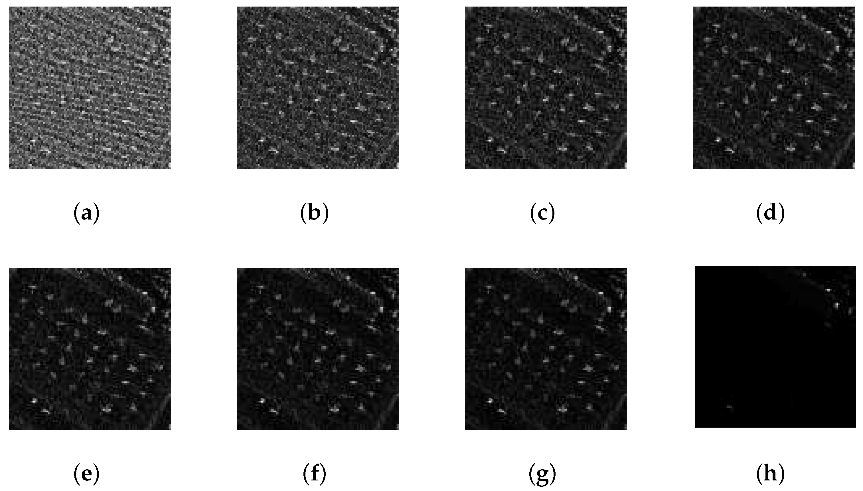
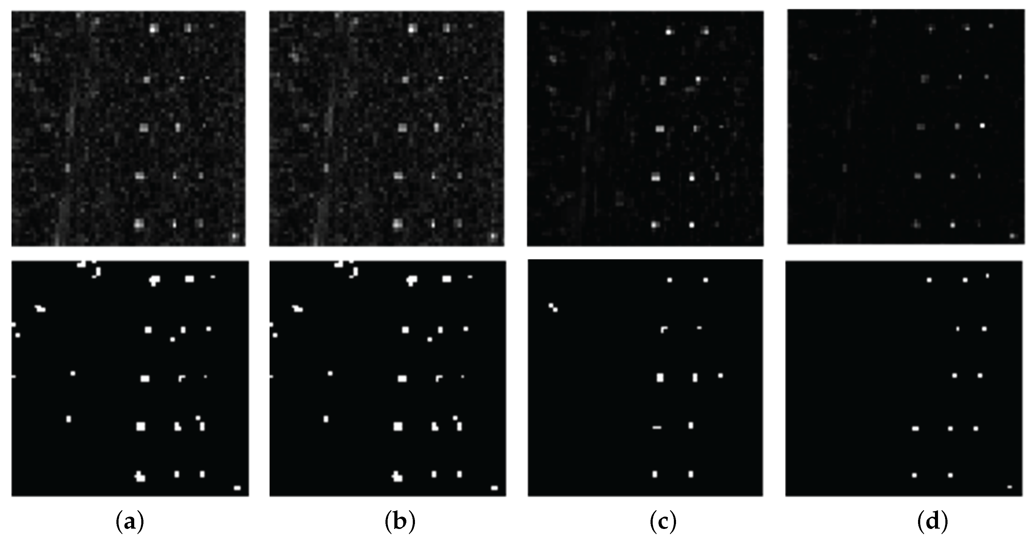
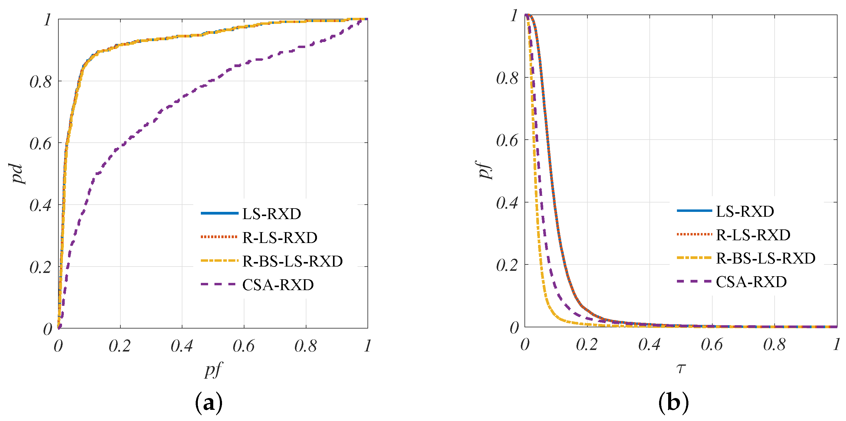
4.2. Performance Evaluation for Different Algorithms

In this section, we compare the detection performance of the LS-RXD, causal sliding array window (CSA-RXD) [18], proposed R-LS-RXD and R-BS-LS-RXD. In order to obtain the best detection results, the sliding window is implemented with size of $13\times 13$ for both AVIRIS and HYDICE hyperspectral images.

Detection results of the four detectors using AVIRIS and HYDICE data are shown in Figure 11 and Figure 12, respectively. The first line shows the gray scale results with detected abundance fractions, and the second line demonstrates the binary detection maps separated in an appropriate threshold, which was calculated by Otsu algorithm [24].

Both hyperspectral images of different sensors came to the same conclusions as follows, showing the adaptation of proposed algorithms for different sensors. It can be found obviously from the detection results that CSA-RXD, which merely take partial advantage of spectral–spatial integration information, omit number targets by visual inspection as shown in Figure 11d and Figure 12d. On the contrary, other anomaly detectors, which are implemented with spectral–spatial integrated information can acquire excellent detection performance. The maximum detection of ground target shows in Figure 6b and Figure 7b can be detected by LS-RXD, R-LS-RXD and R-BS-LS-RXD by visual inspection in Figure 11a–c and Figure 12a–c. As also shown in the figure, R-BS-LS-RXD gets better background suppression compared with R-LS-RXD and LS-RXD. This indicates that R-BS-LS-RXD can not only correctly detect anomaly target pixels as R-LS-RXD performs, but also acquires excellent background suppression as CSA-RXD performs.

Similarly, to simplify our study, a quantitative evaluation with traditional ROC curves, ($Pf$, $\tau$) curves, is demonstrated in Figure 13. AUC values are listed in

Table 5. AUC values with different detectors.

Algorithm	LS-RXD	R-LS-RXD	R-BS-LS-RXD	CSA-RXD
${\mathit{A}}_{\mathit{z}}$ ($\mathit{Pd}$, $\mathit{Pf}$)	0.9286	0.9286	0.9270	0.7401
${\mathit{A}}_{\mathit{z}}$ ($\mathit{Pf}$, $\mathit{\tau }$)	0.0873	0.0873	0.0364	0.0597

, only for AVIRIS Sandiego data, since the results are similar for both data sources.

It is interesting to note that the ROC curves of LS-RXD, R-LS-RXD and R-BS-LS-RXD are overlapped completely. This indicates that these algorithms get similar detection power from the traditional ROC curve analysis. Meanwhile, R-BS-LS-RXD gets a better performance in background suppression as the ($Pf$, $\tau$) curve shows. It is clearly shown that anomaly detectors with spectral–spatial integration have better performance, where the ROC curves of LS-RXD, R-LS-RXD and R-BS-LS-RXD are much closer to the upper left corner than CSA-RXD.

AUC values tablet in Table 5 prove that the proposed R-LS-RXD and R-BS-LS-RXD get a similar detection performance with LS-RXD. In addition, $A_z(Pd,Pf)$ of LS-RXD, R-LS-RXD and R-BS-LS-RXD is greater than CSA-RXD. By contrast, R-BS-LS-RXD produced lowest value of $A_z(Pf,\tau )$. In general, R-BS-LS-RXD can suppress the background information and improve the detection performance.

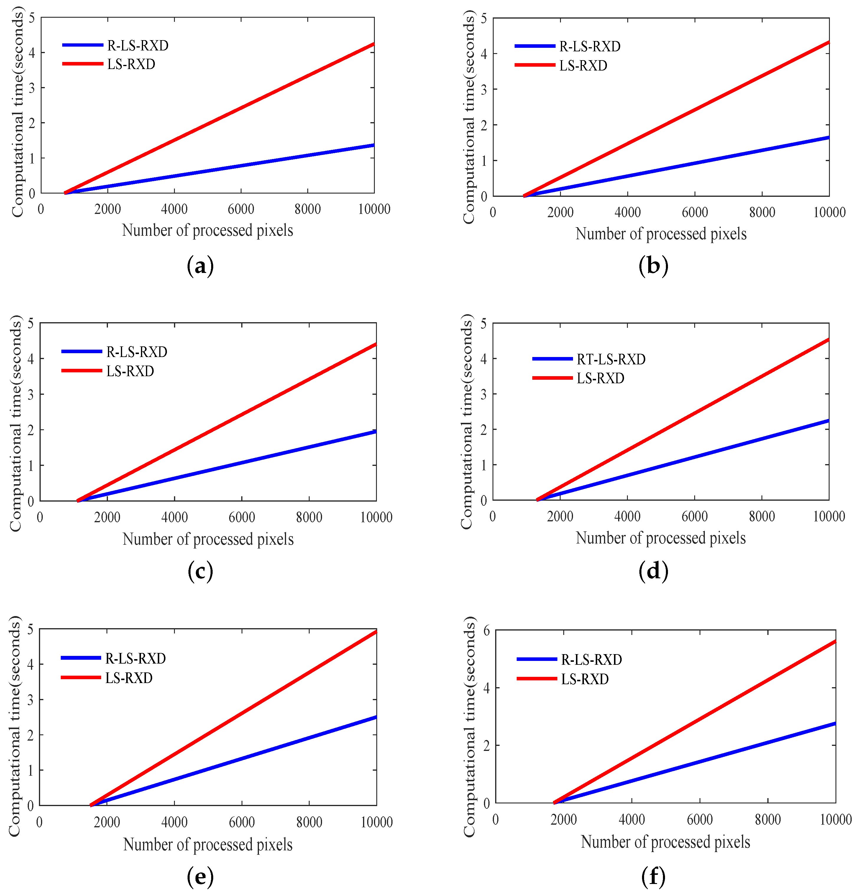
4.3. Computing Time Comparison for Different Algorithms

In order to verify the computing effectiveness of recursive LS-RXD, we design a comprehensive comparative analysis on the computer processing time (CPT) of R-LS-RXD and LS-RXD. The computer environments used for the experiments are 64-bit operating systems with Intel i5-4590, a central processing unit (CPU) of 3.3 GHz, and 8 GB of random access memory (RAM). In order to remove the pulse error caused by the computer itself, the following data on complexity analyses are averaged after five experiments.

Table 6. Computing Time (seconds).

Windowsize	$7\times 7$	$9\times 9$	$11\times 11$	$13\times 13$	$15\times 15$	$17\times 17$
R-LS-RXD	1.366	1.648	1.951	2.247	2.504	2.764
LS-RXD	4.248	4.327	4.407	4.542	4.925	5.618
Speedup	3.110	2.627	2.259	2.022	1.967	2.033

tablets the computing time of algorithms with different window sizes in San Diego hyperspectral image.

Based on the results in Table 6, the computing time of R-LS-RXD is significantly less than LS-RXD in every window size. In addition, the acceleration is particularly noticeable when the window is in a small-scale. In the experiment, the speedup ratio is up to three when the window size is chosen as $7\times 7$. As the window size grows up, the speedup ratio remains, at least, two.

To further evaluate computational complexity, Figure 14 plots the computing time versus the number of processed pixels for both R-LS-RXD and LS-RXD on the Sandiego hyperspectral image. Each algorithm was run and executed five times to produce an average computing time. As we can see, R-LS-RXD requires less time than LS-RXD does due to the fact that the former implements a recursive process, while the latter implements a nonrecursive process. As also shown in the figure, the computing time increases linearly as new pixels are added.

5. Conclusions

This paper proposes a recursive local summation RX algorithm for hyperspectral anomaly detection based on sliding window processing. In order for a fast implementation of a sliding window detector, a recursive update equation for the inversion of local background covariance matrices is developed. In addition, a background suppression R-BS-LS-RXD detector is also proposed in this paper, which removes the current under test pixel from the recursively update processing. This method exploits a local summation strategy in a sliding window, which could sum multiple correlated local background statistics to suppress the major background. The real hyperspectral image experiments have proven that the R-LS-RXD and LS-RXD obtain similar detection performances, which can be competitive with that of CSA-RXD based on sliding array window background. To investigate the computational complexity issue, a comprehensive comparative analysis on the CPT of running recursive updating sliding window detector and un-recursive updating method is conducted in theory and experiments. The result shows R-LS-RXD has a significant acceleration effect for calculation. Our future work mainly focuses on deriving real-time progressive processing of anomaly detection for hyperspectral imagery that was acquired by other data formats.

References

1. Goetz, A.F. Three Decades of Hyperspectral Remote Sensing of The Earth: A Personal View. Remote Sens. Environ. 2009, 113, S5–S16. [Google Scholar] [CrossRef]
2. Chang, C.I. Hyperspectral Data Processing: Algorithm Design and Analysis; Wiley-Interscience: Hoboken, NJ, USA, 2013; pp. 441–442. [Google Scholar]
3. Reed, I.S.; Yu, X. Adaptive Multiple-band CFAR Detection of An Optical Pattern with Unknown Spectral Distribution. IEEE Trans. Acoust. Speech Sign. Proc. 1990, 38, 1760–1770. [Google Scholar] [CrossRef]
4. Nasrabadi, N.M. Hyperspectral Target Detection: An Overview of Current and Future Challenges. IEEE Sign. Proc. Mag. 2014, 31, 34–44. [Google Scholar] [CrossRef]
5. Manolakis, D.; Truslow, E.; Pieper, M.; Cooley, T.; Brueggeman, M. Detection Algorithms in Hyperspectral Imaging Systems: An Overview of Practical Algorithms. IEEE Sign. Proc. Mag. 2014, 31, 24–33. [Google Scholar] [CrossRef]
6. Li, W.; Du, Q. Collaborative Representation for Hyperspectral Anomaly Detection. IEEE Trans. Geosci. Remote Sens. 2015, 53, 1463–1474. [Google Scholar] [CrossRef]
7. Chang, C.I.; Chiang, S.S. Anomaly Detection and Classification for Hyperspectral Imagery. IEEE Trans. Geosci. Remote Sens. 2002, 40, 1314–1325. [Google Scholar] [CrossRef]
8. Chang, C.; Hsueh, M. Characterization of Anomaly Detection in Hyperspectral Imagery. Sensor Rev. 2006, 26, 137–146. [Google Scholar] [CrossRef]
9. Molero, J.M.; Garzón, E.M.; García, I.; Plaza, A. Analysis and Optimizations of Global and Local Versions of the RX Algorithm for Anomaly Detection in Hyperspectral Data. IEEE J. Sel. Top. Appl. Earth Obs. Remote Sens. 2013, 6, 801–814. [Google Scholar] [CrossRef]
10. Liu, W.M.; Chang, C.I. Multiple-Window Anomaly Detection for Hyperspectral Imagery. IEEE J. Sel. Top. Appl. Earth Obs. Remote Sens. 2013, 6, 644–658. [Google Scholar] [CrossRef]
11. Guo, Q.; Zhang, B.; Ran, Q.; Gao, L.; Li, J.; Plaza, A. Weighted-RXD and Linear Filter-Based RXD: Improving Background Statistics Estimation for Anomaly Detection in Hyperspectral Imagery. IEEE J. Sel. Top. Appl. Earth Obs. Remote Sens. 2014, 7, 2351–2366. [Google Scholar] [CrossRef]
12. REN, X.D.; LEI, W.H. Kernel Anomaly Detection Method in Hyperspectral Imagery Based on the Spectral Discrimination Method. Acta Photonica Sin. 2016, 45, 330003. [Google Scholar]
13. Du, B.; Zhao, R.; Zhang, L.P.; Zhang, L.F. A Spectral-spatial Based Local Summation Anomaly Detection Method for Hyperspectral Images. Sign. Proc. 2016, 124, 115–131. [Google Scholar] [CrossRef]
14. Chen, S.Y.; Wang, Y.L.; Wu, C.C.; Liu, C.; Chang, C.I. Real-time Causal Processing of Anomaly Detection for Hyperspectral Imagery. IEEE Trans. Aerosp. Electron. Syst. 2014, 50, 1511–1534. [Google Scholar] [CrossRef]
15. Zhao, C.H.; Wang, Y.L.; Qi, B.; Wang, J. Global and Local Real-Time Anomaly Detectors for Hyperspectral Remote Sensing Imagery. Remote Sens. 2015, 7, 3966–3985. [Google Scholar] [CrossRef]
16. Yang, B.; Yang, M.; Plaza, A.; Gao, L.; Zhang, B. Dual-Mode FPGA Implementation of Target and Anomaly Detection Algorithms for Real-Time Hyperspectral Imaging. IEEE J. Sel. Top. Appl. Earth Obs. Remote Sens. 2015, 8, 2950–2961. [Google Scholar] [CrossRef]
17. Zhang, L.; Peng, B.; Zhang, F.; Wang, L.; Zhang, H.; Zhang, P.; Tong, Q. Fast Real-Time Causal Linewise Progressive Hyperspectral Anomaly Detection via Cholesky Decomposition. IEEE J. Sel. Top. Appl. Earth Obs. Remote Sens. 2017, 10, 4614–4629. [Google Scholar] [CrossRef]
18. Chang, C.I.; Wang, Y.; Chen, S.Y. Anomaly Detection Using Causal Sliding Windows. IEEE J. Sel. Top. Appl. Earth Obs. Remote Sens. 2015, 8, 3260–3270. [Google Scholar] [CrossRef]
19. Zhao, C.H.; Deng, W.W.; Yao, X.F. Hyperspectral Real-Time Anomaly Target Detection Based on Progressive Line Processing. Acta Opt. Sin. 2017, 37, 012800201–012800212. [Google Scholar]
20. Kailath, T. Linear Systems; Prentice-Hall: Upper Saddle River, NJ, USA, 1980; Volume 26, pp. 1–28. [Google Scholar]
21. Wang, Y.L.; Chen, S.Y.; Liu, C.H.; Chang, C.N. Background Suppression Issues in Anomaly Detection for Hyperspectral Imagery. In Proceedings of the Satellite Data Compression, Communications, and Processing X (SPIE), Baltimore, ML, USA, 8–9 May 2014; p. 912413. [Google Scholar]
22. Wang, L.; Chang, C.I.; Lee, L.C.; Wang, Y.; Xue, B.; Song, M.; Yu, C.; Li, S. Band Subset Selection for Anomaly Detection in Hyperspectral Imagery. IEEE Trans. Geosci. Remote Sens. 2017, 55, 4887–4898. [Google Scholar] [CrossRef]
23. Wang, J.; Wang, L.; Cui, J.; Li, X. Band Selection based on Signal-to-noise Ratio Estimation and Hyperspectral Anomaly Detection. Remote Sens. Technol. Appl. 2015, 30, 292–297. [Google Scholar]
24. Otsu, N. A Threshold Selection Method from Gray-Level Histograms. IEEE Trans. Syst. Man Cybern. 1979, 9, 62–66. [Google Scholar] [CrossRef]
Figure 1. Multiple local window filters [13] (a) Window 1. (b) Window 2 and (c) Window 9.
Remotesensing 10 00103 g001
Figure 2. Casual sliding array window at r n with width specified by a.
Remotesensing 10 00103 g002
Figure 3. Sliding window with size of ω × ω .
Remotesensing 10 00103 g003
Figure 4. Sliding window strategy for recursive local summation RXD (R-LS-RXD): (a) N o . ( C o l 2 ) window; (b) N o . ( C o l 1 ) window; (c) N o . C o l window; (d) N o . ( C o l + 1 ) window.
Remotesensing 10 00103 g004
Figure 5. Numbers of floating operations in various of (a) bands; (b) ω size; (c) processed pixels.
Remotesensing 10 00103 g005
Figure 6. Sandiego hyperspectral image (a) 30th band scene; (b) ground truth.
Remotesensing 10 00103 g006
Figure 7. (a) A Hyperspectral Digital Imagery Collection Experiment (HYDICE) panel scene which contains 15 panels; (b) Ground truth map of spatial locations of the 15 panels.
Remotesensing 10 00103 g007
Figure 8. Detection abundance fractional maps of AVIRIS by recursive local summation RXD (R-LS-RXD) with different sliding window size: (a) ω = 5; (b) ω = 7; (c) ω = 9; (d) ω = 11; (e) ω = 13; (f) ω = 15; (g) ω = 17; (h) global.
Remotesensing 10 00103 g008
Figure 9. Detection abundance fractional maps of HYDICE by R-LS-RXD with different sliding window size: (a) ω = 5; (b) ω = 7; (c) ω = 9; (d) ω = 11; (e) ω = 13; (f) ω = 15; (g) ω = 17; (h) global.
Remotesensing 10 00103 g009
Figure 10. Receiver operating characteristic (ROC) curves analysis for AVIRIS data with different window size: (a) curve of ( P d , P f ); (b) curve of ( P f , τ )
Remotesensing 10 00103 g010
Figure 11. Detection results of AVIRIS data for different algorithms: (a) LS-RXD; (b) R-LS-RXD; (c) Recursive background Suppression local summation RXD (R-BS-LS-RXD); (d) Causal sliding array window (CSA-RXD).
Remotesensing 10 00103 g011
Figure 12. Detection results of HYDICE data for different algorithms: (a) LS-RXD; (b) R-LS-RXD; (c) R-BS-LS-RXD; (d) CSA-RXD.
Remotesensing 10 00103 g012
Figure 13. ROC analysis with different detectors: (a) curve of ( P d , P f ); (b) curve of ( P f , τ ).
Remotesensing 10 00103 g013
Figure 14. Plots of computing time versus number of processed pixels. (a) ω = 7; (b) ω = 9; (c) ω = 11; (d) ω = 13; (e) ω = 15; (f) ω = 17.
Remotesensing 10 00103 g014