Superpixel Segmentation of Polarimetric Synthetic Aperture Radar (SAR) Images Based on Generalized Mean Shift

Abstract

The mean shift algorithm has been shown to perform well in optical image segmentation. However, the conventional mean shift algorithm performs poorly if it is directly used with Synthetic Aperture Radar (SAR) images due to the large dynamic range and strong speckle noise. Recently, the Generalized Mean Shift (GMS) algorithm with an adaptive variable asymmetric bandwidth has been proposed for Polarimetric SAR (PolSAR) image filtering. In this paper, the GMS algorithm is further developed for PolSAR image segmentation. A new merging predicate that is defined in the joint spatial-range domain is derived based on the GMS algorithm. A pre-sorting strategy and a post-processing step are also introduced into the GMS segmentation algorithm. The proposed algorithm can be directly used for PolSAR image superpixel segmentation without any pre-processing steps. Experiments using Airborne SAR (AirSAR) and Experimental SAR (ESAR) L-band PolSAR data demonstrate the effectiveness of the proposed superpixel segmentation algorithm. The parameter settings, stability, quality, and efficiency of the GMS algorithm are also discussed at the end of this paper.

1. Introduction

In recent decades, object-based image analysis has become a new paradigm in remote sensing [1,2,3]. Furthermore, in recent years, object-based classification for Polarimetric Synthetic Aperture Radar (PolSAR) images has become more and more popular [4,5,6,7,8,9,10,11,12]. Image segmentation is an important pre-processing step in image interpretation and analysis, and object detection, recognition, and tracking [13]. However, the state-of-the-art segmentation algorithms, such as the Fractal Net Evolution Approach (FNEA) [14], mean shift [13], spectral clustering [15], Simple Linear Iterative Clustering (SLIC) [16], and Statistical Region Merging (SRM) [17], are mostly designed for optical images. It is therefore necessary to develop segmentation algorithms specifically for PolSAR data. To date, various PolSAR image segmentation algorithms have been proposed. These algorithms can be classified into three categories according to the segmentation results, as follows:

(1) Conventional Segmentation Methods. The basic principle of these methods is merging the adjacent and homogeneous pixels into the same region, and dividing the heterogeneous pixels into different regions. The size and shape of the obtained regions vary with the image scenes. Dong et al., [4] proposed using a Gaussian Markov Random Field (GMRF) model for PolSAR image segmentation and classification. For simplicity, this method uses a Gaussian distribution instead of a Gamma distribution, and it only uses the intensity information. Wu et al., [5] proposed to use a Wishart Markov Random Field (WMRF) model and a Maximum A Posteriori (MAP) criterion for PolSAR image segmentation. Compared with the GMRF model, the WMRF model is more in line with the characteristics of PolSAR data. Lombardo et al., [18] derived a split-merge criterion based on a generalized maximum-likelihood approach, and then applied it to multi-frequency PolSAR image segmentation. Ayed et al., [19] proposed to use maximum-likelihood approximation and efficient multiphase level-sets for PolSAR image segmentation. Yin and Yang [20] proposed a modified level-set approach for multi-band PolSAR image segmentation. Zou et al., [21] proposed to use a level-set method based on a heterogeneous cluster model for high-resolution PolSAR image segmentation. Yu et al., [22] introduced the Iterative Region Growing with Semantics (IRGS) algorithm into PolSAR image segmentation and classification by incorporating a polarimetric feature model that is based on the Wishart distribution and modifying several key steps. Lang et al., [23] proposed a Generalized SRM (GSRM) algorithm by modifying the original SRM model according to the characteristics of PolSAR images.

(2) Superpixel Segmentation Methods. These methods segment an image into many small homogeneous regions with similar sizes. The main difference between the conventional segmentation approach and superpixel segmentation is that the latter approach limits the size of the segmented regions (and sometimes may also limit the shape and the edge smoothness). Ersahin et al., [7] introduced the Spectral Graph Partitioning (SGP) algorithm into the PolSAR image processing field for segmentation and classification. Liu et al., [8] first used the polarimetric information to detect edges, and then used the Normalized Cuts (Ncut) [15] algorithm for PolSAR image superpixel segmentation. Spectral clustering methods have good noise immunity, and they can obtain segmented regions with similar sizes, compact shapes, and smooth edges, but they cannot preserve the point and linear objects. Hoekman et al., [6] proposed using the region-growing algorithm for PolSAR image segmentation. This method first initializes some seed points, where each seed point stands for a region. It then divides the adjacent pixels whose distances from the central seed points are less than a certain threshold into the regions for which the central seed points stand. Similar to this method, the SLIC algorithm was introduced into PolSAR image segmentation by Qin et al., [24], where a revised Wishart distance was adopted as the similarity measures. For heterogeneous urban areas, Xiang et al., [25] introduced the Spherically Invariant Random Vectors (SIRV) model. The polarimetric homogeneity measurement that was proposed by Lang et al. [26] was also used to automatically determine the tradeoff factor. Wang et al. further combined the Wishart distance and the SIRV distance [27]. The integrated distance was calculated in a Directional Span-Driven Adaptive (DSDA) region and the superpixels are generated while using the entropy rate method.

(3) Hierarchical Segmentation Methods. These methods, which are also known as multi-scale segmentation methods, produce multi-level segmentation results in top-down or bottom-up order. The top level is the whole image, and the bottom level is a single pixel. All the levels of the segmentation results form a hierarchical structure. Beaulieu et al., [28] proposed a hierarchical stepwise optimal algorithm that is based on the region-merging method for PolSAR image segmentation, where the segmentation criterion was derived from a complex Wishart distribution for homogeneous images and from a K-distribution for texture images. Since the texture model is not unique, Bombrun et al., [29] introduced the SIRV model, which can describe a class of stochastic processes for PolSAR image hierarchical segmentation. To save the segmented results at different levels, Alonso-González et al., [30] proposed the use of Binary Partition Trees (BPT) for PolSAR image multi-scale representation. The two main steps that are involved in BPT analysis are tree construction and tree pruning. Recently, Chen et al., [31] proposed a multi-scale segmentation algorithm for high resolution PolSAR image by introducing superpixel segmentation and the G⁰ distribution statistical heterogeneity into the FNEA algorithm.

This paper focuses on superpixel segmentation. When compared with the conventional segmentation approach, superpixel segmentation can produce small-scale regions with a similar size even in large homogeneous areas, preserving the statistical characteristics of the image. Therefore, superpixel segmentation is more suitable for the object-based classification algorithms that are based on statistics such as the Wishart classifier.

Mean shift segmentation is a commonly used segmentation algorithm. Because the segmentation result of the mean shift algorithm is often piecemeal, it is usually regarded as a superpixel segmentation algorithm. However, the conventional mean shift algorithm is designed only for optical images and cannot be directly used with PolSAR images. Recently, Lang et al., [32] extended the conventional mean shift algorithm according to the characteristics of PolSAR images. The proposed Generalized Mean Shift (GMS) algorithm can be directly used for Synthetic Aperture Radar (SAR) and PolSAR image filtering, avoiding unnecessary information loss. In this paper, the GMS algorithm is further extended for the superpixel segmentation of PolSAR images.

The main contributions of this paper are as follows: (1) We propose a new merging predicate to be used for superpixel segmentation based on the basic GMS formula, and we further propose the GMS algorithm based on the new merging predicate. (2) To improve the accuracy of the segmentation, we introduce a pre-sorting strategy into the GMS segmentation algorithm after comparing the pre-sorting strategy and the row-column strategy used in the conventional mean shift segmentation algorithm. (3) To suppress the influence of speckle noise and preserve strong point targets, we introduce a post-processing step into the GMS segmentation algorithm.

The rest of this paper is organized as follows. Firstly, in Section 2, we briefly review the materials and methods that are used in this study. A new merging predicate defined in the joint spatial-range domain is derived based on the GMS algorithm. A pre-sorting strategy and a post-processing step are introduced into the GMS segmentation algorithm. Section 3 describes the experimental results that were obtained with AirSAR and ESAR L-band PolSAR data and evaluates the effectiveness of the proposed algorithm. The parameter settings, stability, quality, and efficiency of the GMS segmentation algorithm are discussed in Section 4. Finally, in Section 5, we conclude the paper and summarize the next steps in this work.

2. Materials and Methods

2.1. Experimental Data Sets and Preprocessing

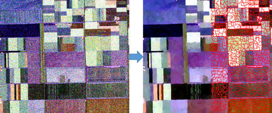
NASA/JPL Airborne SAR (AirSAR) and DLR Experimental SAR (ESAR) L-band PolSAR data were selected to evaluate the effectiveness of the proposed superpixel segmentation algorithm by comparison with the original mean shift algorithm [13], the normalized cuts (Ncut) algorithm used in [8], and the SLIC-PolSAR algorithm using the grid-centered initialization strategy (SLIC-GC) [24]. The data sets that were used in this study are freely available from the website of the European Space Agency (ESA) (https://earth.esa.int/web/polsarpro/airborne-data-sources). Because the Ncut and SLIC-GC algorithms are sensitive to speckle noise, filtering processing is required before the segmentation step. In these experiments, the PolSAR data were preprocessed by the refined Lee filter [33]. The GMS segmentation algorithm involves the GMS filtering process, so no extra filtering processing was needed. The first data set was a four-look AirSAR L-Band PolSAR image from Flevoland, the Netherlands. Since the original image was as large as 750 × 1024, for the convenience of showing details of the image, a region of 380 × 430, which was as the same as the one shown in Figure 9 in [8], was sampled from the original image. Because the points and lines in the image were small and fine, a speckle filter with a large window might have blurred the points, lines, and edges, which are very important in remote sensing image segmentation, so we used a relatively small window, 3 × 3, for the refined Lee filter. The Red-Green-Blue color image composited by Pauli decomposition parameters (Pauli-RGB image) of this area is shown in Figure 1a, and the 3 × 3 refined Lee filtered image is shown in Figure 1b. Since the filtering window was small, strong speckle noise can still be observed in Figure 1b.

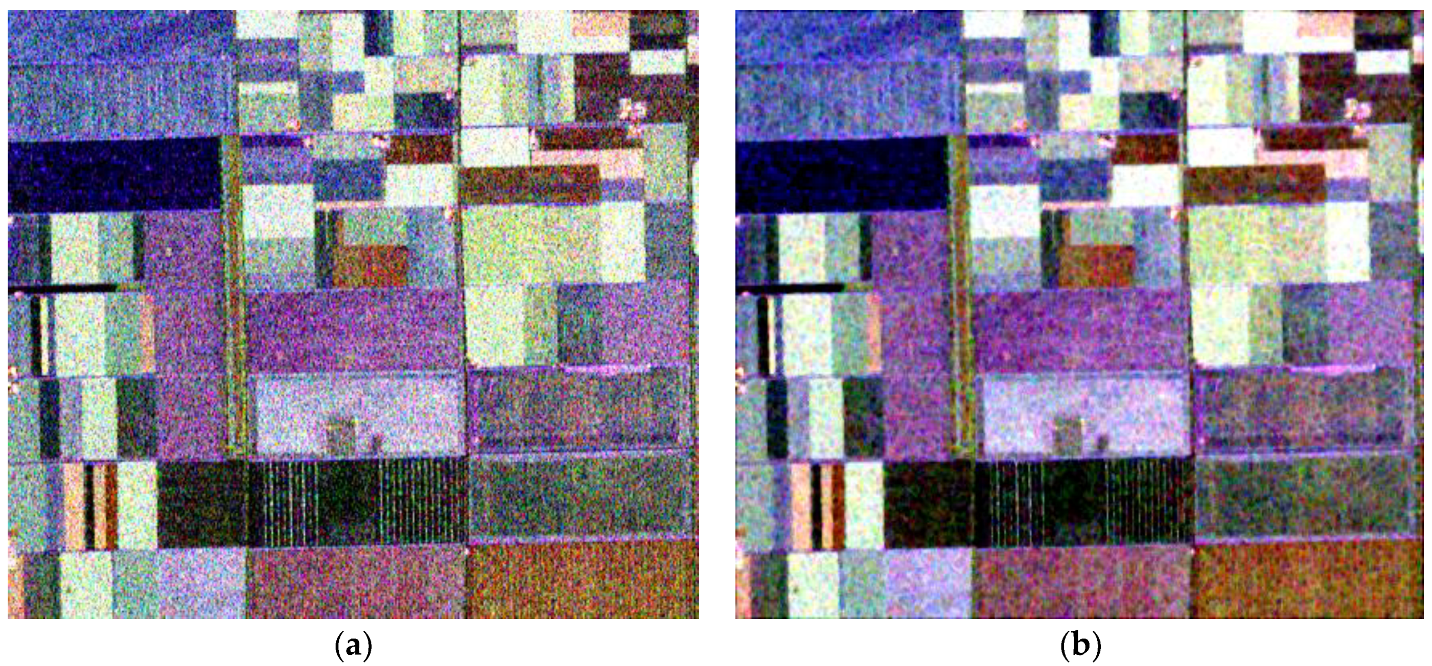
The second data set was an ESAR L-band PolSAR image from the Oberpfaffenhofen test site, Germany. The original single-look image was 2861 × 1540 in size. To facilitate the visual interpretation and evaluation, a pre-processing of two looks in the azimuth direction was performed to equalize the resolutions of the azimuth and range, and a region of 540 × 888, which was the same as the one shown in Figure 9 in [32], was sampled from the original image. Since the points and lines in the ESAR image were bigger and thicker than those in the AirSAR image, and the speckle noise of the former was stronger than the latter, we chose a 7 × 7 window for the refined Lee filter. The Pauli-RGB image of this area is shown in Figure 2a, and the 7 × 7 refined Lee filtered image is shown in Figure 2b. It can be observed from Figure 2 that the speckle noise is well suppressed, but some details are blurred, such as the dark lines in the areas that are marked by the ellipse.

2.2. Conventional Mean Shift Segmentation

2.2.1. Conventional Mean Shift

The mean shift procedure was proposed for nonparametric density gradient estimation by Fukunaga and Hostetler [34], and it was improved and applied to data and image analysis, including smoothing, segmentation, clustering, and real-time tracking of objects by Cheng [35] and Comaniciu et al., [13,36,37,38,39]. The following is a brief introduction to the conventional mean shift algorithm.

Given n independent and identically distributed (i.i.d.) random vectors x_i ∈R^d, i = 1, …, n, in the d-dimensional space R^d, the PDF of x_i can be estimated by the multivariate kernel density estimator with kernel K(x) and a symmetric positive definite d × d bandwidth matrix H:

$$\widehat{f}(x)=\frac{1}{n}{\displaystyle \sum _{i=1}^n{K}_H\left(x-x_i\right)}$$

(1)

Where

$$K_H(x)={\left|H\right|}^{-1/2}K\left(H^{-1/2}x\right)$$

(2)

In practice, to reduce the complexity of the estimation, the bandwidth matrix H is chosen as proportional to the identity matrix H = h²I. In pattern recognition, a special class of radially symmetric kernels satisfying $K(x)=c_{k}k\left({\Vert x\Vert }^2\right)$ are usually used, where the function k(x) is called the kernel profile, and constant c_k makes the integral of K(x) equal to one. Accordingly, the PDF estimator (Equation (1)) can be rewritten as:

$${\widehat{f}}_{h,K}(x)=\frac{c_k}{n{h}^d}{\displaystyle \sum _{i=1}^{n}k\left({\Vert \frac{x-x_i}{h}\Vert }^2\right)}$$

(3)

A key step in the feature space analysis with the underlying density f(x) is to find the local maximum values of the density, i.e., the modes of the density. For a continuous PDF, the modes are located where the gradient ∇f(x) = 0. The mean shift procedure is an efficient way to locate these modes without estimating the PDF. The mean shift vector is calculated, as follows [13]:

$$M_{h,Q}(x)=\frac{{\displaystyle \sum _{i=1}^n{x}_{i}q\left({\Vert \frac{x-x_i}{h}\Vert }^2\right)}}{{\displaystyle \sum _{i=1}^{n}q\left({\Vert \frac{x-x_i}{h}\Vert }^2\right)}}-x$$

(4)

where q(x) = −k’(x) and Q(x) = c_qq(||x||²). The kernel K(x) was called the shadow of the kernel Q(x) in [35]. From Equation (4), it can be found that the mean shift vector is the difference between the weighted mean of the area bounded by bandwidth h and the center point x. At each point, the mean shift vector always points to the direction of maximum increase of f(x), so it can define a path leading to a mode of f(x). The mean shift procedure is defined as an iterative process. At each iteration, the mean shift vector (Equation (4)) is calculated and it is added to the center point to obtain the new center until it converges to a mode point where the density gradient is zero.

2.2.2. Mean Shift Filtering

In order to take full advantage of the spatial information that is contained in the image, Comaniciu and Meer [13] proposed introducing a multivariate kernel that is defined in the joint spatial-range domain into the mean shift procedure:

$$K_{h_s,h_r}(x)=\frac{C}{h_s{}^2{h}_r{}^d}{k}_s\left({\Vert \frac{x_s}{h_s}\Vert }^2\right)k_r\left({\Vert \frac{x_r}{h_r}\Vert }^2\right)$$

(5)

where x_s is the spatial part, x_r is the range part of feature vector x, k_s(x) and k_r(x) are the profiles used in the two domains, h_s and h_r are the employed kernel bandwidths, and C is the corresponding normalization constant.

Mean shift filtering is a straightforward application of the mean shift procedure. For each point x defined in the d-dimensional space, find its mode point x_m by using the mean shift iterative process, and assign the filtered value of x = (x_s, x_m,r).

2.2.3. Mean Shift Segmentation

The principle of the conventional mean shift segmentation is straightforward [13]: firstly, run the mean shift filtering procedure for the image and store both the spatial and range information of the mode point; then, merge the pixels whose mode points’ spatial distances are less than h_s and range distances are less than h_r.

We suppose that x_k and z_k (k = [1, N]) are the d-dimensional pixels in the original input image I and the filtered image I_f defined in the joint spatial-range domain, and L_i is the region label that the i-th pixel belongs to. The procedure of the conventional mean shift segmentation algorithm can then be described, as follows:

Algorithm 1. Mean Shift Segmentation Algorithm

Run the mean shift filtering procedure for the image I, obtain the filtered image If, and save the coordinate of each pixel’s mode point. Judge the adjacent pixels in turn. Merge the pixels in If whose mode points’ spatial distances are less than hs and range distances are less than hr. (Optional) Merge the small regions whose sizes are less than M pixels into the most similar adjacent regions. Suppose that the number of final segmented regions is m, and the segmented regions are Cp, p = 1,…,m. For each pixel k = 1,…,N, assign Lk = { p | zk$\in$Cp}.

From the procedure of mean shift segmentation, it can be seen that this algorithm uses the region growing and merging technique, which contains two elements: the merging predicate confirming whether adjacent regions are merged or not, and the merging order followed to test the merging of regions. In this paper, the mean shift segmentation algorithm is improved from these two aspects, so that it is appropriate for PolSAR images.

2.3. Generalized Mean Shift Segmentation

2.3.1. Generalized Mean Shift

It is known that the probability distribution of single-look and N-look amplitude SAR data is asymmetric, as is the intensity. However, the bandwidth of the conventional mean shift algorithm is symmetric. Furthermore, a single fixed bandwidth is also inadequate, since the range of SAR data is usually very large. Therefore, pre-processing, such as logarithmic transformation and normalization, has to be applied before the mean shift filter is used for SAR images in the existing approaches [40,41,42,43]. Clearly, these pre-processing steps will result in a loss of some information and reduce the segmentation quality. To overcome these problems, Lang et al., [32] proposed using an adaptive variable asymmetric bandwidth, and derived the GMS:

$$M_G(x)=\frac{{\displaystyle \sum _{i=1}^{n}q\left({\Vert \frac{x-x_i}{h(x)}\Vert }^2\right)x_i}}{{\displaystyle \sum _{i=1}^{n}q\left({\Vert \frac{x-x_i}{h(x)}\Vert }^2\right)}}-x$$

(6)

where x = [x₁, x₂,…, x_p] is the center pixel in an image with p channels, x_i is a sample pixel, q(||x||²) is the profile of the kernel function Q(x), and h(x) is the bandwidth vector:

$$h=\{\begin{array}{l}{h}_{j,1}=\left(1-{\sigma }_1\right){\widehat{x}}_j,if{x}_{i,j}\le x_j\\ h_{j,2}=\left({\sigma }_2-1\right){\widehat{x}}_j,if{x}_{i,j}>x_j\end{array},1\le j\le p$$

(7)

where ${\widehat{x}}_j$ is the Minimum Mean Square Error (MMSE) [44,45] estimated value of the center pixel in channel j, and (σ₁, σ₂) is the sigma range that maintains the mean value of the SAR intensity or amplitude [32,46]. Since the sigma range was described by parameter ξ in [46], the bandwidth vector h is determined only by parameter ξ.

If we suppose that a = [a₁,a₂,…,a_n] and b = [b₁,b₂,…,b_n] are two n-dimensional vectors, then the vector division a/b is defined as:

$$\frac{a}{b}=\left[\frac{a_1}{b_1},\dots ,\frac{a_n}{b_n}\right]$$

(8)

According to Equations (7) and (8), the Euclidean norm used in the profile function is:

$${\Vert \frac{x-x_i}{h}\Vert }^2={\displaystyle \sum {\left(\frac{x_j-x_{i,j}}{h_{j,1}}\right)}^2}+{\displaystyle \sum {\left(\frac{x_k-x_{i,k}}{h_{k,2}}\right)}^2}$$

(9)

where the subscript j stands for the dimension x_i,j≤x_j, and the subscript k stands for the dimension x_i,k>x_k, in the total p range dimensions. For more information about GMS, we refer the reader to [32]. After the above extension, the GMS algorithm can be used directly with SAR data without any pre-processing steps.

Accordingly, we obtain the new GMS that is defined in the joint spatial-range domain:

$$M_G\left(x\right)=\frac{{\displaystyle \sum _{i=1}^n{q}_s\left({\Vert \frac{x_{i,s}-x_s}{h_s}\Vert }^2\right)q_r\left({\Vert \frac{x_{i,r}-x_r}{h(x_r)}\Vert }^2\right)x_i}}{{\displaystyle \sum _{i=1}^n{q}_s\left({\Vert \frac{x_{i,s}-x_s}{h_s}\Vert }^2\right)q_r\left({\Vert \frac{x_{i,r}-x_r}{h(x_r)}\Vert }^2\right)}}-x$$

(10)

where subscripts s and r stand for the spatial and range domains, respectively.

2.3.2. Merging Predicate

The merging predicate of the conventional mean shift segmentation can be defined in mathematical form as:

$$P\left(z,z_i\right)=\{\begin{array}{cc}true.& if\left(\Vert z_{i,s}-z_s\Vert <h_s\right)\&\left(\Vert z_{i,r}-z_r\Vert <h_r\right)\\ false.& otherwise\end{array}$$

(11)

where z denotes the center pixel filtered by the mean shift filter and z_i denotes an adjacent pixel.

The conventional mean shift defined in the joint spatial-range domain is [32]:

$$M_{h_s,h_r,Q}\left(x\right)=\frac{{\displaystyle \sum _{i=1}^n{q}_s\left({\Vert \frac{x_{i,s}-x_s}{h_s}\Vert }^2\right)q_r\left({\Vert \frac{x_{i,r}-x_r}{h_r}\Vert }^2\right)x_i}}{{\displaystyle \sum _{i=1}^n{q}_s\left({\Vert \frac{x_{i,s}-x_s}{h_s}\Vert }^2\right)q_r\left({\Vert \frac{x_{i,r}-x_r}{h_r}\Vert }^2\right)}}-x$$

(12)

By comparing Equations (11) and (12), the predicate (Equation (11)) can be modified, as follows:

$$P\left(z,z_i\right)=\{\begin{array}{cc}true.& if\left(\Vert \frac{z_{i,s}-z_s}{h_s}\Vert <1\right)\&\left(\Vert \frac{z_{i,r}-z_r}{h_r}\Vert <1\right)\\ false.& otherwise\end{array}$$

(13)

Equation (13) indicates that the merging predicate of the mean shift segmentation algorithm is judging whether the parameter of the profile function q(x) is less than 1 or not.

Accordingly, the merging predicate of the GMS segmentation algorithm can be derived based on Equation (10):

$$P_G\left(z,z_i\right)=\{\begin{array}{cc}true.& if\left(\Vert \frac{z_{i,s}-z_s}{h_s}\Vert <1\right)\&\left(\Vert \frac{z_{i,r}-z_r}{h(z_r)}\Vert <1\right)\\ false.& otherwise\end{array}$$

(14)

What we should note here is, that, differing from mean shift, during the region-merging process of GMS, two regions are involved, whose corresponding range bandwidths are h(x) and h(x_i), respectively. However, only the bandwidth of the central pixel is considered in Equation (14), which is not comprehensive. We therefore need to consider how to use these two bandwidths. In general, there are four main approaches: (1) minimum; (2) maximum; (3) summation; and, (4) difference. The fourth method can be eliminated because the result is a constant, which can be derived according to Equation (7). The final bandwidths of the other three methods increase from (1) to (3). Since the bigger the bandwidth, the higher the merging probability, we choose the first method to reduce the over-merging problem. Accordingly, the predicate (Equation (14)) becomes:

$$P_G\left(z,z_i\right)=\{\begin{array}{cc}true.& if\left(\Vert \frac{z_{i,s}-z_s}{h_s}\Vert <1\right)\&\left(\Vert \frac{z_{i,r}-z_r}{\min \left(h(z_r),h(z_{i,r})\right)}\Vert <1\right)\\ false.& otherwise\end{array}$$

(15)

In the conventional mean shift segmentation algorithm, the adjacent pixels are used to decide if the regions to which the adjacent pixels belong to should be merged. However, this model might produce unsatisfactory results since the value of a single pixel may not be true in a noise-polluted image. To ensure the reliability of the merging test, the adjacent homogeneous pixels should be used to estimate the central pixel. For a segmentation algorithm that is based on the region-growing and merging technique, the pixels in the same segmented region are considered to be homogenous. Therefore, any pixel in the same region can be represented by the mean of the region. In this paper, the means of two adjacent regions are used to judge if they should be merged. Consequently, the merging predicate (Equation (15)) becomes:

$$P_G\left(\mathrm{R}(z),\mathrm{R}(z_i)\right)=\{\begin{array}{cc}true.& if\left(\Vert \frac{z_{i,s}-z_s}{h_s}\Vert <1\right)\&\left(\Vert \frac{\overline{{\mathrm{R}}_r(z_i)}-\overline{{\mathrm{R}}_r(z)}}{\min \left(h\left(\overline{{\mathrm{R}}_r(z)}\right),h\left(\overline{{\mathrm{R}}_r(z_i)}\right)\right)}\Vert <1\right)\\ false.& otherwise\end{array}$$

(16)

where R(z) stands for the region to which pixel z belongs and $\overline{{\mathrm{R}}_r(z)}$ stands for the mean values of region R in the range domain.

2.3.3. Merging Order

From Equation (16), we can deduce that the merging order will influence the merging result, because the mean region value will be different if the merging order is changed. In the conventional mean shift segmentation algorithm, the merging predicate is tested in row-column order. This strategy can obtain correct segmentation results when the borders between different classes are clear, but when the borders are ambiguous, the results may be wrong. For example, in Figure 3a, where the border of class 1 and class 2 is clear, the row-column strategy can obtain two regions that are consistent with class 1 and class 2. However, in Figure 3b, where the border is ambiguous, class 1 and class 2 are merged into one region (Figure 4a), even if the bandwidth is set as small as 15.

However, it is clear that the smaller the difference of the merged pixels, the better the reliability of the merging predicate. Therefore, we propose to use a pre-sorting strategy that first sorts the adjacent pixel pairs according to their difference or gradient in increasing order, and it then traverses this order only once [17,23]. For any current pair of pixels (p₁,p₂), if R(p₁) ≠ R(p₂), we make the test P_G(R(p₁),R(p₂)) and merge R(p₁) and R(p₂) if the result is true.

When using the pre-sorting strategy, the adjacent pixels with the smallest differences in Figure 3b will be merged first. The border pixels will be later merged into several different regions, as shown in Figure 4b–d. We can see that, even when the bandwidth is set as high as 90, class 1 and class 2 can be preserved.

Since the pre-sorting strategy sorts the differences or gradients of adjacent pixels, the gradient function should be deduced according to Equation (15), and not Equation (16). On the basis of Equation (15), the gradient function used for sorting is:

$$f(z,z_i)=\Vert \frac{z_r-z_{i,r}}{\min \left(h(z_r),h(z_{i,r})\right)}\Vert$$

(17)

2.3.4. Post-Processing

As with most segmentation algorithms, the result of mean shift segmentation is often very broken due to the influence of speckle noise. A post-processing step is therefore needed to eliminate the “noisy regions”, which are composed of only one or several pixels.

The strategy of the post-processing is usually straightforward: merge the regions whose sizes are less than a threshold N_n into their nearest neighbors [13]. However, this strategy might result in some small heterogeneous objects being merged inappropriately, which is not conducive to the follow-up image interpretation. To preserve strong point targets while eliminating the noisy regions, we adopt the same strategy as [24]: set a threshold N_p, whose value should be set manually, according to the size of the point targets in the PolSAR image. Any region less than N_p is directly merged into its most similar adjacent region as a noisy region. If the size of a region is in the range of [N_p, N_n), the gradient of the region and its nearest neighbor should be calculated. If the gradient is bigger than a threshold G_th, the region is preserved as a strong point target; else, merge the two regions. The gradient measure used in this paper is defined, as follows [23,24]:

$$G\left(R_i,R_j\right)=\frac{1}{q}{\Vert \frac{T_i^{diag}-T_j^{diag}}{T_i^{diag}+T_j^{diag}}\Vert }_1$$

(18)

where T^diag denotes the vector that is composed by the diagonal elements of the central coherence matrix T of a region R, ${\Vert ·\Vert }_1$ denotes the 1-norm, and q is the number of diagonal elements. Since the range of G is [0,1], it is simple to set the threshold G_th. In this study, we set G_th = 0.2 in all of the experiments.

2.3.5. GMS Superpixel Segmentation for PolSAR Data

Because the GMS segmentation method is used to produce superpixels, the size of the maximum superpixel should be controlled during the region merging. If we suppose that the size threshold of the maximum superpixel is N_max, then the complete procedure of the proposed GMS superpixel segmentation algorithm can be summarized, as follows:

Algorithm 2. Generalized Mean Shift (GMS) Superpixel Segmentation Algorithm

1. GMS filtering 1) Let x and z be the d-dimensional input and filtered image pixels in the joint spatial-range domain, xi, i = 1,..., n are the adjacent pixels of x, and yj, j = 1, 2,..., to which the successive locations of the mean shift vectors point. Given an initial point x, assign j=1 and yj = x. 2) From Equation (10), yj+1 can be calculated by: $$y_{j+1}=\frac{{\displaystyle \sum _{i=1}^n{q}_s\left({\Vert \frac{x_{i,s}-x_s}{h_s}\Vert }^2\right)q_r\left({\Vert \frac{x_{i,r}-x_r}{h(x_r)}\Vert }^2\right)x_i}}{{\displaystyle \sum _{i=1}^n{q}_s\left({\Vert \frac{x_{i,s}-x_s}{h_s}\Vert }^2\right)q_r\left({\Vert \frac{x_{i,r}-x_r}{h(x_r)}\Vert }^2\right)}}$$ (19) and the j-th GMS vector can be written as: >Mj = yj+1 − yj. (20) 3) If Mj < ε, then yj+1 is the mode point, assign z = (xs, yj+1,r) and break; else, assign yj = yj+1 and j = j + 1, go to step 2), and compute the new yj+1 and Mj. 2. GMS merging 1) Let SI be the set of adjacent pixel pairs in I in the 8-neighborhood. Compute the gradients of the pairs in SI by Equation (17). 2) Sort the pairs of SI by the gradients computed in Step 1) in increasing order. 3) In the series of SI, for any current pair (z, zi) ∈ SI, if R(z) = R(zi), compute the merging criterion PG(R(z), R(zi)) by Equation (16). If the result is true, and their total size is less than Nmax, merge R(z) and R(zi). 3. Post-processing. For each segmented region, if its size Ns is less than Nn, compute the gradient between this region and its neighboring regions. Find the minimum gradient Gmin. If Gmin < Gth or Ns < Np, merge the two regions; else, set the region aside.

It should be noted that, in Algorithm 2, the spatial bandwidths used in the GMS filtering step (denoted by h_s^f) and the GMS merging step (denoted by h_s^m) are different. h_s^f means the radius of the filtering window, and it is a positive integer that is equal to or greater than 1. Meanwhile, h_s^m means the spatial location threshold of the mode points, and it is a positive real number that is usually assigned as equal to or less than 1. In this study, we set h_s^f = 5 and h_s^m = 1 in all of the experiments.

3. Results

3.1. Evaluation Based on AirSAR Data

Firstly, Figure 1a was processed by the original mean shift segmentation algorithm with h_s = 7, M = 10, and h_r = 10, 15, and 20, respectively. The results are shown in Figure 5a–c, with the right halves of the figures showing the borders of the segmented regions. The obtained numbers of regions are N_r = 6474, 5467, and 3444, respectively. From the left halves of Figure 5a–c, it can be clearly seen that the points and edges in Figure 1a are not preserved well. From the right halves of Figure 5a–c, both over-segmentation and over-merging can be clearly observed, as in the area that is marked by the rectangle. The over-segmentation could be reduced by parameter adjustment, while the over-merging situation would increase, and vice versa. To further understand the results, the mean shift filtered images are shown in Figure 5d–f, from which we can see that the speckle noise is barely suppressed, especially in dark areas, such as the areas that are marked by the ellipses.

The GMS superpixel segmentation algorithm was then applied to the AirSAR PolSAR image. The filtering and merging parameters were set as: ξ = 0.9, h_s^f = 5, h_s^m = 1, and N_max = 100. Although there are several other parameters that need to be set, the appropriate values have been discussed in [32]. These values were directly selected as the default values. The post-processing parameters were set as: N_n = 49, N_p = 4, and G_th = 0.2. The result is shown in Figure 6a, with N_r = 2021. When compared with Figure 5a–c, Figure 6a presents a better segmentation quality: the sizes of the superpixels are similar, the borders of the superpixels are smoother, and the points and edges are preserved well, proving the effectiveness of the GMS superpixel segmentation algorithm.

For comparison, the Ncut algorithm was applied to the first data set. The desired superpixel number was set as k = 2000. The result is shown in Figure 6b, with N_r = 2016. From a general view, the left half of Figure 6b is similar to the left half of Figure 6a. However, the right half of Figure 6b shows that the Ncut superpixels are more compact and the shapes and sizes of the superpixels are more similar. On the other hand, the points and lines, such as those that are marked by the red ellipses, are not preserved well.

Finally, the SLIC-GC algorithm was applied to the AirSAR PolSAR image. The desired superpixel number was again set as k = 2000. The post-processing parameters were the same as for the GMS algorithm. The result is shown in Figure 6c, with N_r = 2081. When compared with Figure 6a and Figure 6b, the left half of Figure 6c shows that the segmentation result is broken and discontinuous in homogeneous areas, and both the edges of homogeneous areas and the borders of superpixels are jagged, such as those areas that are marked by the rectangles. This indicates that the SLIC-GC algorithm is still affected by speckle noise. In addition, the compactness of Figure 6c is m = 0.5. When this parameter is set as a larger value, the superpixels are more compact, but the points and lines are not preserved. When it is set as a smaller value, the shapes of the superpixels are more irregular, and the borders are more jagged.

To further evaluate the segmentation quality, the ratio method that was used in [47] was adopted. The first step is to obtain the ratio images of the original intensity image to the segmented versions. Based on the ratio images, there are two ways to evaluate the segmentation quality:

1) Qualitative evaluation: This method is a visual evaluation method used to evaluate the ability of a segmentation algorithm in detail preservation. If the ratio image is made up of random noise without structured information, it can be considered that the segmentation result depicts the ideal segmentation image; otherwise, any sign of structure indicates a loss of detail.

2) Quantitative evaluation: The mean and variance of the ratio image are calculated. For the intensity ratio image, the theoretical mean value is $\overline{r}$ = 1, and the theoretical variance is given by:

$$\mathrm{var}(r)=\frac{1}{N-1}{\displaystyle \sum _{j=1}^m\frac{n_j}{L+\left(1/n_j\right)}}$$

(21)

where N is the number of pixels in the ratio image, m is the number of segments, n_j is the number of pixels in the j-th segment, and L is the number of looks. The closer the mean value to the theoretical one, the better the radiometric information preservation ability. Since the value of any segment is defined as the local average, the mean value of the ratio image is always 1. Similarly, the closer the variance to the theoretical one, the better the detail information preservation ability.

The ratio images of the original image to the segmented versions of the different algorithms are shown in Figure 7, being plotted over the range [0.5, 1.5]. Weak structural information can be observed in Figure 7a,c, indicating the good detail preservation abilities of the GMS and SLIC-GC algorithms. Meanwhile, strong and obvious structures can be observed in Figure 7b, indicating the poor detail preservation ability of the Ncut algorithm.

The quantitative evaluation measurements of the superpixel segmentation results are listed in

Table 1. Means and variances of the ratio images for the different superpixel segmentation algorithms with the AirSAR image.

Algorithm	Number of Superpixels	Mean	Variance	Theoretical Variance
GMS	2021	1.0	0.2645	0.2492
Ncut	2016	1.0	0.3278	0.2492
SLIC-GC	2081	1.0	0.2549	0.2492

. Although the numbers of superpixels are different, the theoretical variances are equal. The variance of the SLIC-GC segmentation is the smallest and it is the closest to the theoretical value. The GMS result is close to the SLIC-GC, which is consistent with the visual assessment. The variance of the Ncut segmentation is the biggest.

The execution efficiency is always an important evaluation measurement for a segmentation algorithm. The execution times of the different superpixel segmentation algorithms are listed in

Table 2. Execution times of the different superpixel segmentation algorithms with the AirSAR image.

Algorithm	Filtering(s)	Segmentation(s)	Total(s)	Execution Environment
GMS	30	1	31	Windows 10 x64, Intel(R) Core(TM) i7-4710MQ CPU @ 2.50 GHz, RAM: 8.0 GB
Ncut	1	218	219
SLIC-GC	1	11	12

. Since all three algorithms need filtering steps, the execution times of both the filtering and segmentation steps are taken into account. Table 2 shows that although the GMS algorithm has an obvious advantage in the segmentation step, it has a moderate performance in total execution time due to the low efficiency of the GMS filter. The most efficient segmentation algorithm is SLIC-GC. The execution time of the Ncut algorithm is far more than other algorithms.

3.2. Evaluation Based on ESAR Data

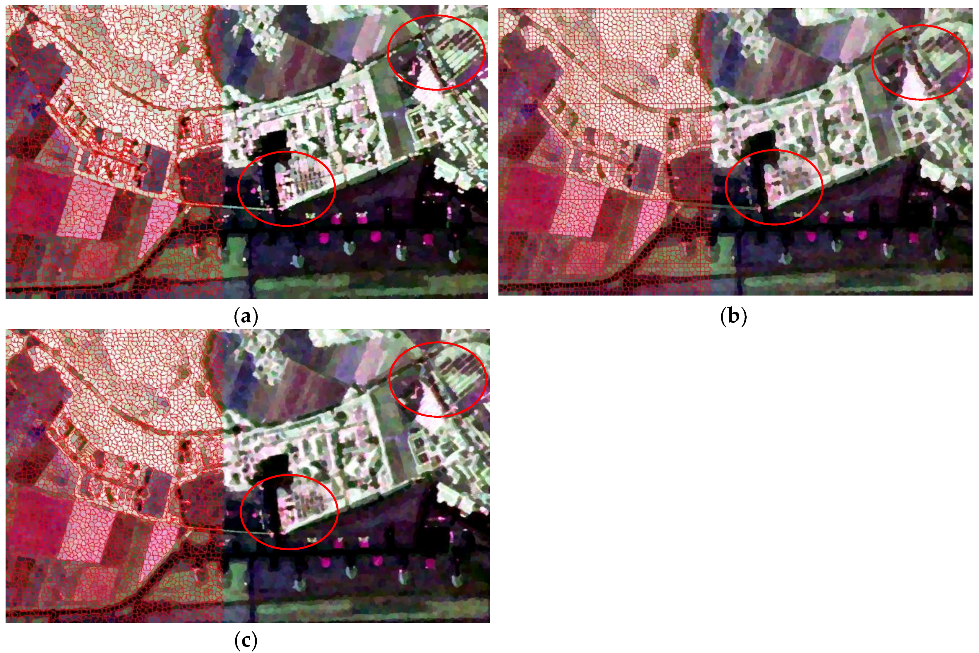
Figure 8 shows the visual assessment of the GMS superpixel segmentation algorithm, the Ncut segmentation algorithm, and the SLIC-GC segmentation algorithm applied to the ESAR image. For the GMS superpixel segmentation algorithm, the filtering, merging, and post-processing parameters were the same as for the first data set. The result is shown in Figure 8a, with N_r = 7449. From the right side of Figure 8a, we can see that the points and lines in the image are preserved well, such as those in the areas that are marked by the ellipses. From the left side of Figure 8a, it can be observed that the sizes and shapes of the superpixels are irregular and they vary with the different scenes.

For the Ncut algorithm, the desired superpixel number was set as k = 8000. The result is shown in Figure 8b, with N_r = 8064. From the left side of Figure 8b, it can be seen that the sizes and shapes of the superpixels are regular, and the borders are smooth. However, the right side of Figure 8b shows that the points and lines are blurred obviously, especially those in the areas that are marked by the ellipse, although the number of superpixels is larger than that of the GMS algorithm.

For the SLIC-GC algorithm, the desired superpixel number was also set as k = 8000. The post-processing parameters were the same as for the first data set. The result is shown in Figure 8c, with N_r = 7728. When compared with Figure 2a, the right side of Figure 8c shows a moderate segmentation quality, since some dark lines and bright points in the areas marked by the ellipse are not preserved well. However, when compared with Figure 2b, Figure 8c can be considered as acceptable. The right side is similar to Figure 2b, and the left side shows that the sizes and shapes of the superpixels are similar, and the borders of the superpixels are smooth, due to the good speckle noise suppression. When combined with the experimental results that were obtained with the first data set, we can conclude that the SLIC-GC algorithm is sensitive to speckle noise, and its segmentation quality depends on the performance of the filtering algorithm.

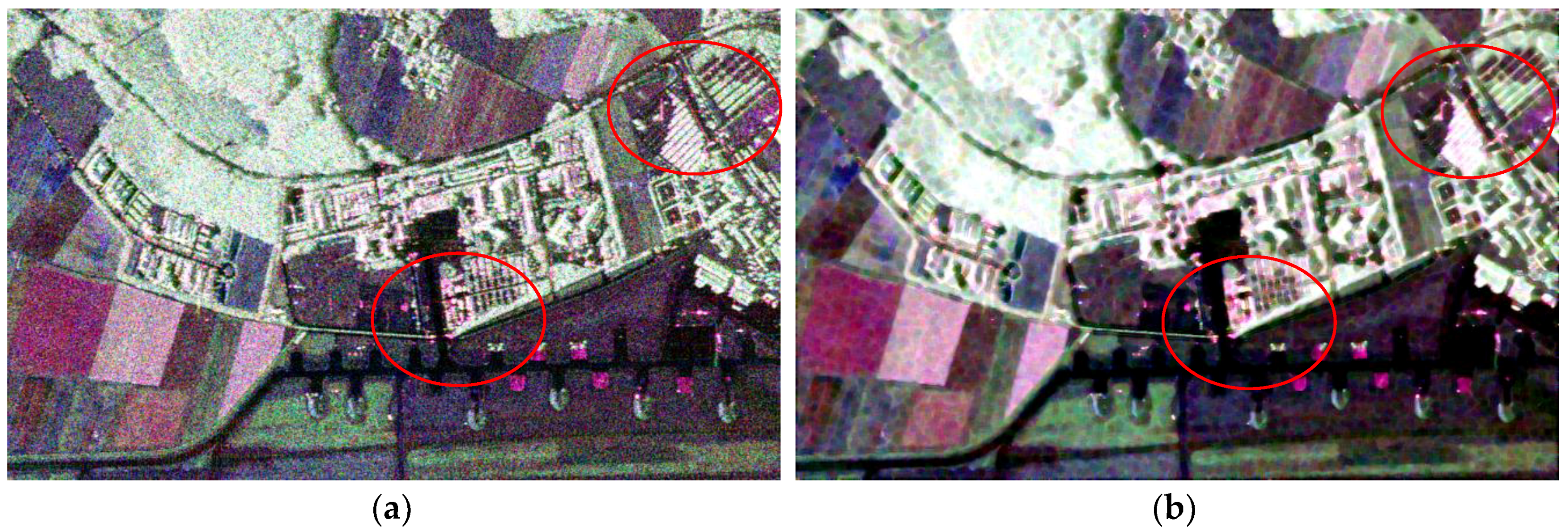
The ratio method was again used to evaluate the segmentation quality. The ratio images of the different algorithms are shown in Figure 9, being plotted over the range [0.5, 1.5]. Similar to the first data set, weak structural information can be observed in Figure 9a,c, and strong and obvious structures can be observed in Figure 9b, indicating the good detail preservation abilities of the GMS and SLIC-GC algorithms, and the poor detail preservation ability of the Ncut algorithm.

The quantitative evaluation measurements are listed in

Table 3. Means and variances of the ratio images for the different superpixel segmentation algorithms with the ESAR image.

Algorithm	Number of Superpixels	Mean	Variance	Theoretical Variance
GMS	7449	1.0	0.5293	0.4963
Ncut	8064	1.0	0.9545	0.4959
SLIC-GC	7728	1.0	0.5723	0.4961

. Since the differences of the numbers of superpixels are much bigger than the first data set, the theoretical variances are different, but they are very close. From Table 3, we can find that the variance of the GMS segmentation is the smallest and it is the closest to the theoretical value. The SLIC-GC result is slightly worse. The variance of the Ncut segmentation is nearly twice the theoretical value.

The execution times of the different superpixel segmentation algorithms are listed in

Table 4. Execution times of the different superpixel segmentation algorithms with the ESAR image.

Algorithm	Filtering(s)	Segmentation(s)	Total(s)	Execution Environment
GMS	306	4	310	Windows 10 x64, Intel(R) Core(TM) i7-4710MQ CPU @ 2.50 GHz, RAM: 8.0 GB
Ncut	4	250	254
SLIC-GC	4	40	44

. Table 4 shows that the GMS algorithm still has an obvious advantage in the segmentation step. However, due to the low efficiency of the GMS filter, the total execution time of the GMS algorithm is the longest.

Combined with the first data set, we can find that, when the number of looks is high or the speckle noise is not very strong, the SLIC-GC algorithm has the best segmentation results. When the speckle noise is strong, the SLIC-GC algorithm gets worse, and the GMS algorithm get better. In the aspect of execution efficiency, the GMS algorithm has an obvious advantage in the segmentation step. However, the efficiency of the GMS filter is too low. The GMS algorithm does not have any advantage in the total execution time. How to improve the efficiency of GMS filtering is an urgent problem to be solved. Since this problem is beyond the scope of this paper, limited discussion will be expressed in Section 4.2.

4. Discussion

4.1. Parameter Settings

It is well known that the parameter settings are of great importance to a segmentation algorithm. There are many parameters that are involved in the GMS algorithm. However, as analyzed in [32], most of the parameters have strong adaptability in the appropriate range. A set of default parameters can nearly always obtain good results for different data. In practical applications, the parameters can be set to the default values. The parameter settings of the filtering step used in this paper were the same as those in [32], except that h_s^f was set to 5. The reason for this is that a filtering algorithm with a small window is more efficient and it can preserve more details, which is helpful to subsequent segmentation.

The new parameters of the merging step are {h_s^m, N_max, N_n, N_p, G_th}. Among them, h_s^m is usually set to 1 by default. The other four parameters have nothing to do with the segmentation algorithm, but are dependent on the application requirements and the actual situation of the images. N_max and N_n are related to the desired size or amount of segmented regions. Suppose that the total number of pixels is N_I, the excepted size of the segmented regions is S, and the expected number of the segmented regions is N_S. They have the follow relationship: N_I = S * N_S. The empirical value of N_max can be set in the range (S, 2S] or (S, 2N_I/N_S]. The empirical value of N_n can be set in the range [S/4, S) or [N_I/4N_S, S). It should be noted that, due to the presence of some small heterogeneous regions, the actual number of segmented regions N_a is often larger than N_s. By increasing N_max and N_n, N_a can be close to or even less than N_S. N_p is related to the minimum target size in the image. When the image resolution is high and the point target is large, N_p should be set as a large value, and vice versa. G_th reflects the heterogeneity degree of the same class of objects in the image. G_th should be set as a large value when the difference between the same class of objects is large. When the difference between different objects in the image is small, G_th should be set as a small value. When both situations occur at the same time, priority should be given to the second situation, which is to set a small value for G_th to ensure the homogeneity of pixels within the same segmented region.

4.2. Stability and Efficiency

The stability of segmentation algorithms was discussed in [48], and a stable mean shift algorithm was proposed. The so-called stable segmentation algorithm means that a segmentation algorithm should get matching results for any two overlapping subsets of an image. The basic mean shift segmentation algorithm is considered to be stable according to the analysis in [48]. However, some optimization steps can lead to instability of the mean shift algorithm. Therefore, the proposed stable version in fact achieves the stabilization of the mean shift process by giving up the optimization steps, so as to realize the image tile segmentation. Finally, the execution efficiency of the mean shift segmentation could be improved by the use of parallel computing technology.

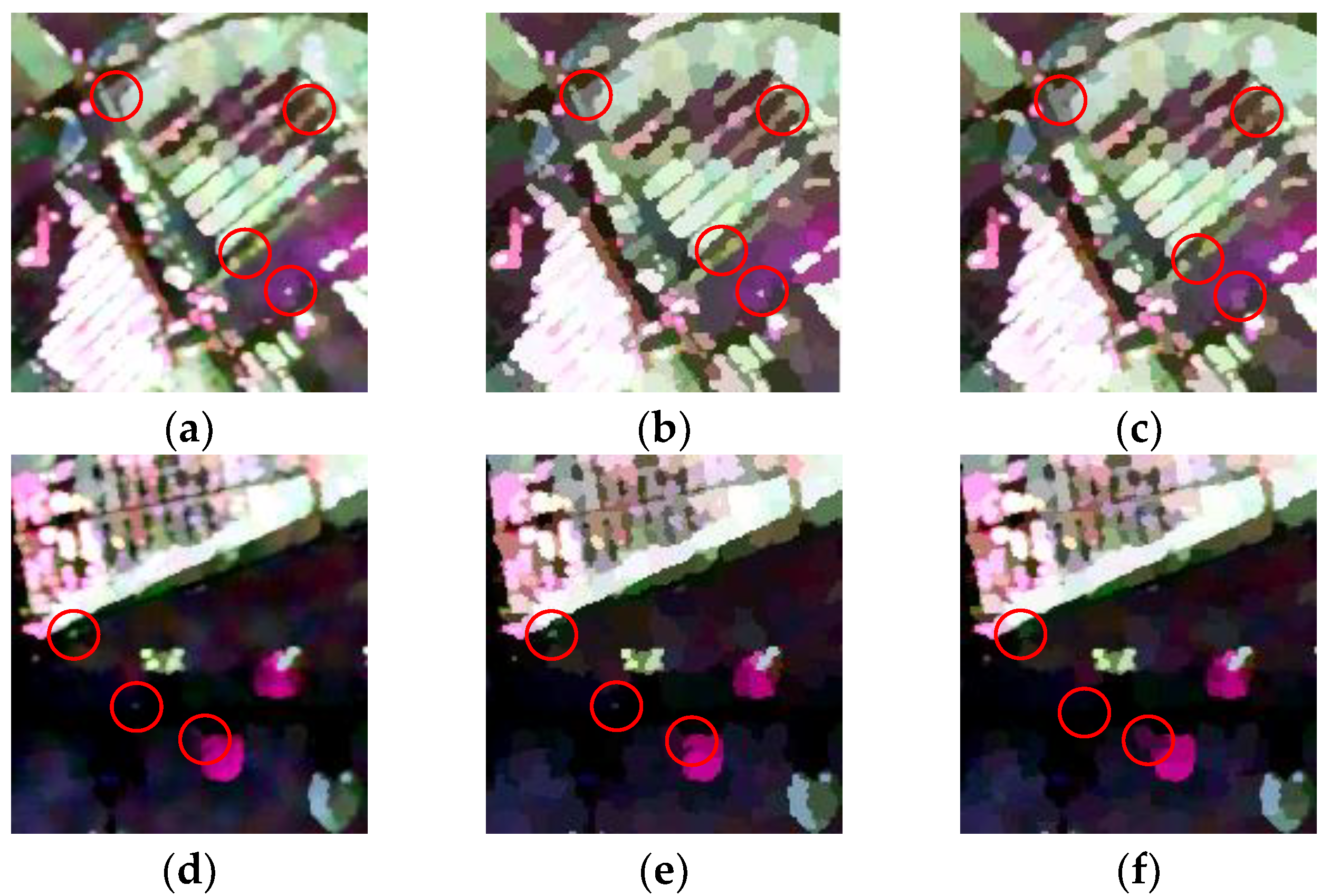
The GMS segmentation algorithm that is proposed in this paper is unstable because it adopts a pre-sorting strategy, and different tile partition methods lead to different orders. According to [48], the GMS segmentation algorithm can also have a corresponding stable version, i.e., with the optimization strategies, such as the pre-sorting strategy and the post-processing step not adopted. However, this may result in a decline of the segmentation quality. In order to obtain a better balance between segmentation quality and efficiency, another experiment was undertaken. Figure 10 shows the GMS segmentation results with and without the pre-sorting strategy and the post-processing step, and the filtering results are also shown. The obtained number of regions for the GMS algorithm without the pre-sorting strategy and the post-processing step (GMS-0 for short) is N_r = 73511, which is nearly 10 times larger than the result that is shown in Figure 8a. The execution time of the GMS-0 segmentation is less than 2s. The areas that are marked by the circle in Figure 10 show that some of the points, edges, and lines that are preserved well by the proposed GMS algorithm are not preserved by the GMS-0 algorithm, even though the obtained superpixels of the latter are nearly 10 times the size of the former. As it is well known that both effectiveness and efficiency are important to an algorithm, when we cannot have both, we should make a choice that is based on the actual requirements.

5. Conclusions

The work that is proposed in this paper is an extension of the previous work by Lang et al., [32], who proposed the GMS algorithm and applied it to PolSAR image filtering. In this paper, the GMS algorithm is further applied to PolSAR image superpixel segmentation. A new merging predicate defined in the joint spatial-range domain is derived based on the GMS algorithm. A pre-sorting strategy and a post-processing step are also introduced into the GMS segmentation algorithm. When compared with the conventional mean shift segmentation algorithm, the method proposed in this paper can be directly applied to PolSAR images without any pre-processing. The experimental results that were obtained with AirSAR and ESAR L-band PolSAR data showed that the GMS segmentation algorithm has good anti-noise ability and can preserve the detail information by producing superpixels conforming to the actual scene of the image. Although the GMS, Ncut, and SLIC-GC algorithms all require pre-processing filtering to suppress speckle noise, the GMS segmentation is bound to the GMS filtering, and thus show a robust performance. For the Ncut and SLIC-GC algorithms, different choices of filters and filtering parameters can produce very different segmentation results.

The time consumption of the GMS filtering is longer than the other algorithms due to the low efficiency of the GMS iterative process. Although the segmentation efficiency could be improved by abandoning the optimization steps and adopting parallel computing technology, the segmentation quality might decline. How to achieve a balance between segmentation quality and efficiency for the GMS algorithm is still an open research topic.

References

- Blaschke, T.; Lang, S.; Hay, G.J. (Eds.) Object-Based Image Analysis: Spatial Concepts for Knowledge-Driven Remote Sensing Applications; Lecture Notes in Geoinformation and Cartography; Springer: Berlin/Heidelberg, Germany, 2008; ISBN 978-3-540-77058-9. [Google Scholar]
- Blaschke, T. Object based image analysis for remote sensing. ISPRS J. Photogramm. Remote Sens. 2010, 65, 2–16. [Google Scholar] [CrossRef]
- Blaschke, T.; Hay, G.J.; Kelly, M.; Lang, S.; Hofmann, P.; Addink, E.; Queiroz Feitosa, R.; van der Meer, F.; van der Werff, H.; van Coillie, F.; et al. Geographic Object-Based Image Analysis—Towards a new paradigm. ISPRS J. Photogramm. Remote Sens. 2014, 87, 180–191. [Google Scholar] [CrossRef] [PubMed]
- Dong, Y.; Milne, A.K.K.; Forster, B.C.C. Segmentation and Classification of Vegetated Areas Using Polarimetric SAR Image Data. IEEE Trans. Geosci. Remote Sens. 2001, 39, 321–329. [Google Scholar] [CrossRef]
- Wu, Y.; Ji, K.; Yu, W.; Su, Y. Region-Based Classification of Polarimetric SAR Images Using Wishart MRF. IEEE Geosci. Remote Sens. Lett. 2008, 5, 668–672. [Google Scholar] [CrossRef]
- Hoekman, D.H.; Vissers, M.A.M.; Tran, T.N. Unsupervised Full-Polarimetric SAR Data Segmentation as a Tool for Classification of Agricultural Areas. IEEE J. Sel. Top. Appl. Earth Obs. Remote Sens. 2011, 4, 402–411. [Google Scholar] [CrossRef]
- Ersahin, K.; Cumming, I.G.; Ward, R.K. Segmentation and Classification of Polarimetric SAR Data Using Spectral Graph Partitioning. IEEE Trans. Geosci. Remote Sens. 2010, 48, 164–174. [Google Scholar] [CrossRef] [Green Version]
- Liu, B.; Hu, H.; Wang, H.; Wang, K.; Liu, X.; Yu, W. Superpixel-Based Classification with an Adaptive Number of Classes for Polarimetric SAR Images. IEEE Trans. Geosci. Remote Sens. 2013, 51, 907–924. [Google Scholar] [CrossRef]
- Qi, Z.; Yeh, A.G.-O.; Li, X.; Lin, Z. A novel algorithm for land use and land cover classification using RADARSAT-2 polarimetric SAR data. Remote Sens. Environ. 2012, 118, 21–39. [Google Scholar] [CrossRef]
- Ma, X.; Shen, H.; Yang, J.; Zhang, L.; Li, P. Polarimetric-Spatial Classification of SAR Images Based on the Fusion of Multiple Classifiers. IEEE J. Sel. Top. Appl. Earth Obs. Remote Sens. 2014, 7, 961–971. [Google Scholar] [CrossRef]
- Jiao, X.; Kovacs, J.M.; Shang, J.; McNairn, H.; Walters, D.; Ma, B.; Geng, X. Object-oriented crop mapping and monitoring using multi-temporal polarimetric RADARSAT-2 data. ISPRS J. Photogramm. Remote Sens. 2014, 96, 38–46. [Google Scholar] [CrossRef]
- Zhang, Y.; Zhang, J.; Zhang, X.; Wu, H.; Guo, M. Land Cover Classification from Polarimetric SAR Data Based on Image Segmentation and Decision Trees. Can. J. Remote Sens. 2015, 41, 40–50. [Google Scholar] [CrossRef]
- Comaniciu, D.; Meer, P.; Member, S. Mean Shift: A Robust Approach toward Feature Space Analysis. IEEE Trans. Pattern Anal. Mach. Intell. 2002, 24, 603–619. [Google Scholar] [CrossRef]
- Baatz, M.; Schape, A. Multiresolution Segmentation: An optimization approach for high quality multi-scale image segmentation. J. Photogramm. Remote Sens. 2000, 58, 12–23. [Google Scholar]
- Shi, J.; Malik, J. Normalized cuts and image segmentation. IEEE Trans. Pattern Anal. Mach. Intell. 2000, 22, 888–905. [Google Scholar] [CrossRef] [Green Version]
- Achanta, R.; Shaji, A.; Smith, K.; Lucchi, A.; Fua, P.; Süsstrunk, S. SLIC Superpixels Compared to State-of-the-Art Superpixel Methods. IEEE Trans. Pattern Anal. Mach. Intell. 2012, 34, 2274–2282. [Google Scholar] [CrossRef] [PubMed] [Green Version]
- Nock, R.; Nielsen, F. Statistical Region Merging. IEEE Trans. Pattern Anal. Mach. Intell. 2004, 26, 1452–1458. [Google Scholar] [CrossRef] [PubMed]
- Lombardo, P.; Sciotti, M.; Pellizzeri, T.M.; Meloni, M. Optimum model-based segmentation techniques for multifrequency polarimetric SAR images of urban areas. IEEE Trans. Geosci. Remote Sens. 2003, 41, 1959–1975. [Google Scholar] [CrossRef]
- Ben Ayed, I.; Mitiche, A.; Belhadj, Z. Polarimetric image segmentation via maximum-likelihood approximation and efficient multiphase level-sets. IEEE Trans. Pattern Anal. Mach. Intell. 2006, 28, 1493–1500. [Google Scholar] [CrossRef] [PubMed]
- Yin, J.; Yang, J. A Modified Level Set Approach for Segmentation of Multiband Polarimetric SAR Images. IEEE Trans. Geosci. Remote Sens. 2014, 52, 7222–7232. [Google Scholar] [CrossRef]
- Zou, P.; Li, Z.; Tian, B.; Guo, L. A level set method for segmentation of high-resolution polarimetric SAR images using a heterogeneous clutter model. Remote Sens. Lett. 2015, 6, 548–557. [Google Scholar] [CrossRef]
- Yu, P.; Qin, A.K.; Clausi, D.A.; Member, S. Unsupervised Polarimetric SAR Image Segmentation and Classification Using Region Growing With Edge Penalty. IEEE Trans. Geosci. Remote Sens. 2012, 50, 1302–1317. [Google Scholar] [CrossRef]
- Lang, F.; Yang, J.; Li, D.; Zhao, L.; Shi, L. Polarimetric SAR Image Segmentation Using Statistical Region Merging. IEEE Geosci. Remote Sens. Lett. 2014, 11, 509–513. [Google Scholar] [CrossRef]
- Qin, F.; Guo, J.; Lang, F. Superpixel Segmentation for Polarimetric SAR Imagery Using Local Iterative Clustering. IEEE Geosci. Remote Sens. Lett. 2015, 12, 13–17. [Google Scholar] [CrossRef]
- Xiang, D.; Ban, Y.; Wang, W.; Su, Y. Adaptive Superpixel Generation for Polarimetric SAR Images with Local Iterative Clustering and SIRV Model. IEEE Trans. Geosci. Remote Sens. 2017, 55, 3115–3131. [Google Scholar] [CrossRef]
- Lang, F.; Yang, J.; Li, D. Adaptive-Window Polarimetric SAR Image Speckle Filtering Based on a Homogeneity Measurement. IEEE Trans. Geosci. Remote Sens. 2015, 53, 5435–5446. [Google Scholar] [CrossRef]
- Wang, W.; Xiang, D.; Ban, Y.; Zhang, J.; Wan, J. Superpixel Segmentation of Polarimetric SAR Images Based on Integrated Distance Measure and Entropy Rate Method. IEEE J. Sel. Top. Appl. Earth Obs. Remote Sens. 2017, 10, 4045–4058. [Google Scholar] [CrossRef]
- Beaulieu, J.-M.; Touzi, R. Segmentation of textured polarimetric SAR scenes by likelihood approximation. IEEE Trans. Geosci. Remote Sens. 2004, 42, 2063–2072. [Google Scholar] [CrossRef]
- Bombrun, L.; Vasile, G.; Gay, M.; Totir, F. Hierarchical Segmentation of Polarimetric SAR Images Using Heterogeneous Clutter Models. IEEE Trans. Geosci. Remote Sens. 2011, 49, 726–737. [Google Scholar] [CrossRef] [Green Version]
- Alonso-gonzález, A.; López-martínez, C.; Salembier, P. Filtering and Segmentation of Polarimetric SAR Data Based on Binary Partition Trees. IEEE Trans. Geosci. Remote Sens. 2012, 50, 593–605. [Google Scholar] [CrossRef]
- Chen, Q.; Li, L.; Xu, Q.; Yang, S.; Shi, X.; Liu, X. Multi-feature segmentation for high-resolution polarimetric SAR data based on fractal net evolution approach. Remote Sens. 2017, 9, 570. [Google Scholar] [CrossRef]
- Lang, F.; Yang, J.; Li, D.; Shi, L.; Wei, J. Mean-Shift-Based Speckle Filtering of Polarimetric SAR Data. IEEE Trans. Geosci. Remote Sens. 2014, 52, 4440–4454. [Google Scholar] [CrossRef]
- Fukunaga, K.; Hostetler, L. The estimation of the gradient of a density function, with applications in pattern recognition. IEEE Trans. Inf. Theory 1975, 21, 32–40. [Google Scholar] [CrossRef]
- Cheng, Y. Mean Shift, Mode Seeking, and Clustering. IEEE Trans. Pattern Anal. Mach. Intell. 1995, 17, 790–799. [Google Scholar] [CrossRef]
- Comaniciu, D.; Meer, P. Mean shift analysis and applications. In Proceedings of the IEEE International Conference on Computer Vision (ICCV), Kerkyra, Greece, 20–27 September 1999; Volume 2, pp. 1197–1203. [Google Scholar]
- Comaniciu, D.; Ramesh, V.; Meer, P. Real-time tracking of non-rigid objects using mean shift. In Proceedings of the IEEE Conference on Computer Vision and Pattern Recognition (CVPR), Hilton Head Island, SC, USA, 13–15 June 2000; Volume 2, pp. 142–149. [Google Scholar]
- Comaniciu, D.; Ramesh, V.; Meer, P. The variable bandwidth mean shift and data-driven scale selection. In Proceedings of the IEEE International Conference on Computer Vision (ICCV 2001), Vancouver, BC, Canada, 7–14 July 2001; IEEE Computer Society: Vancouver, BC, Canada, 2001; Volume 1, pp. 438–445. [Google Scholar]
- Comaniciu, D. An algorithm for data-driven bandwidth selection. IEEE Trans. Pattern Anal. Mach. Intell. 2003, 25, 281–288. [Google Scholar] [CrossRef] [Green Version]
- Cellier, F.; Oriot, H.; Nicolas, J.M. Introduction of the mean shift algorithm in SAR imagery: Application to shadow extraction for building reconstruction. In Proceedings of the IEEE International Workshop on Biomedical Circuits and Systems, Singapore, 1–3 December 2004. [Google Scholar]
- Jarabo-Amores, P.; Rosa-Zurera, M.; Mata-Moya, D.; Vicen-Bueno, R. “Mean-Shift” filtering to reduce speckle noise in SAR images. In Proceedings of the IEEE Intrumentation and Measurement Technology Conference, Singapore, 5–7 May 2009; pp. 1188–1193. [Google Scholar]
- Beaulieu, J.; Touzi, R. Mean-Shift and Hierarchical Clustering for Textured Polarimetric SAR Image Segmentation/Classification. In Proceedings of the IEEE IGARSS 2010, Honolulu, HI, USA, 25–30 July 2010; pp. 2519–2522. [Google Scholar]
- Jarabo-Amores, P.; Rosa-Zurera, M.; de la Mata-Moya, D.; Vicen-Bueno, R.; Maldonado-Bascon, S. Spatial-Range Mean-Shift Filtering and Segmentation Applied to SAR Images. IEEE Trans. Instrum. Meas. 2011, 60, 584–597. [Google Scholar] [CrossRef]
- Lee, J.-S. Digital Image Enhancement and Noise Filtering by Use of Local Statistics. IEEE Trans. Pattern Anal. Mach. Intell. 1980, 165–168. [Google Scholar] [CrossRef] [Green Version]
- Kuan, D.T.; Sawchuk, A.A.; Member, S.; Strand, T.C.; Chavel, P. Adaptive Noise Smoothing Filter for Images with Signal-Dependent Noise. IEEE Trans. Pattern Anal. Mach. Intell. 1985, 165–177. [Google Scholar] [CrossRef]
- Lee, J.; Wen, J.; Ainsworth, T.L.; Chen, K.; Chen, A.J. Improved Sigma Filter for Speckle Filtering of SAR Imagery. IEEE Trans. Geosci. Remote Sens. 2009, 47, 202–213. [Google Scholar] [CrossRef]
- Lee, J.S.J.; Grunes, M.R.M.R.; De Grandi, G.; Member, S.; De Grandi, G. Polarimetric SAR speckle filtering and its implication for classification. IEEE Trans. Geosci. Remote Sens. 1999, 37, 2363–2373. [Google Scholar] [CrossRef]
- Oliver, C.; Quegan, S. Understanding Synthetic Aperture Radar Images; SciTech Publishing, Inc.: Raleigh, NC, USA, 2004; ISBN 1-891121-31-6. [Google Scholar]
- Michel, J.; Youssefi, D.; Grizonnet, M. Stable Mean-Shift Algorithm and Its Application to the Segmentation of Arbitrarily Large Remote Sensing Images. IEEE Trans. Geosci. Remote Sens. 2015, 53, 952–964. [Google Scholar] [CrossRef]
Figure 1.
Pauli-RGB images of the Airborne Synthetic Aperture Radar (AirSAR) Polarimetric SAR (PolSAR) data: (a) Original image and (b) 3×3 refined Lee filtered image.
Figure 2.
Pauli-RGB images of the Experimental Synthetic Aperture Radar (ESAR) PolSAR data: (a) Original image and (b) 7 × 7 refined Lee filtered image.
Figure 3.
Class 1 and class 2 with (a) clear and (b) ambiguous borders.
Figure 4.
Mean shift segmentation results of Figure 3b using (a) the row-column strategy with range bandwidth h = 15 and 30 (same result); and, (b)–(d) the pre-sorting strategy with range bandwidth h = 30, 60, and 90, respectively.
Figure 5.
The segmentation (a–c) and filtering (d–f) results of the conventional mean shift algorithm with hs = 7, M = 10, and hr = 10 (a,d), hr = 15 (b,e), and hr = 20 (c,f).
Figure 6.
The superpixel segmentation results obtained with the AirSAR PolSAR image: (a) GMS segmentation, with Nr = 2021; (b) Ncut segmentation, with Nr = 2016; and, (c) Simple Linear Iterative Clustering algorithm for PolSAR image with the grid-centered initialization strategy (SLIC-GC) segmentation, with Nr = 2081.
Figure 7.
The ratio images of the different superpixel segmentation algorithms for the AirSAR PolSAR image: (a) GMS segmentation, with Nr = 7449; (b) Ncut segmentation, with Nr = 8064; and, (c) SLIC-GC segmentation, with Nr = 7728.
Figure 8.
The superpixel segmentation results that were obtained with the ESAR PolSAR image: (a) GMS segmentation, with Nr = 7449; (b) Ncut segmentation, with Nr = 8064; and, (c) SLIC-GC segmentation, with Nr = 7728.
Figure 9.
The ratio images of the different superpixel segmentation algorithms for the ESAR PolSAR image: (a) GMS segmentation, with Nr= 7449; (b) Ncut segmentation, with Nr= 8064; and, (c) SLIC-GC segmentation, with Nr= 7728.
Figure 10.
The GMS filtering and segmentation results of the ESAR PolSAR image. (a) and (d) are the filtering results. (b) and (e) are the segmentation results with the pre-sorting strategy and the post-processing step. (c) and (f) are the segmentation results without the pre-sorting strategy and the post-processing step.