Monitoring Population Evolution in China Using Time-Series DMSP/OLS Nightlight Imagery


1
Institute of Remote Sensing and Digital Earth, Chinese Academy of Sciences, Beijing 100101, China
2
University of Chinese Academy of Sciences, Beijing 100049, China
*
Author to whom correspondence should be addressed.
Remote Sens. 2018, 10(2), 194; https://doi.org/10.3390/rs10020194
Submission received: 16 November 2017
/
Revised: 17 January 2018
/
Accepted: 26 January 2018
/
Published: 28 January 2018
Abstract
:Accurate and detailed monitoring of population distribution and evolution is of great significance in formulating a population planning strategy in China. The Defense Meteorological Satellite Program’s Operational Linescan System (DMSP/OLS) nighttime lights time-series (NLT) image products offer a good opportunity for detecting the population distribution owing to its high correlation to human activities. However, their detection capability is greatly limited owing to a lack of in-flight calibration. At present, the synergistic use of systematically-corrected NLT products and population spatialization is rarely applied. This work proposed a methodology to improve the application precision and versatility of NLT products, explored a feasible approach to quantitatively spatialize the population to grid units of , and revealed the spatio-temporal characteristics of population distribution from 2000 to 2010. Results indicated that, (1) after inter-calibration, geometric, incompatibility and discontinuity corrections, and adjustment based on vegetation information, the incompatibility and discontinuity of NTL products were successfully solved. Accordingly, detailed actual residential areas and luminance differences between the urban core and the peripheral regions could be obtained. (2) The population spatialization method could effectively acquire population information at per with high accuracy and exhibit more details in the evolution of population distribution. (3) Obvious differences in spatio-temporal characteristics existed in four economic regions, from the aspects of population distribution and dynamics, as well as population-weighted centroids. The eastern region was the most populous with the largest increased magnitude, followed by the central, northeastern, and western regions. The population-weighted centroids of the eastern, western, and northeastern regions moved along the southwest direction, while the population-weighted centroid of the central region moved along the southeast direction. (4) The population distribution and dynamics in nine-level population density types were significantly different. In the period of 2000–2010, the population in the basic no-man and high concentration types presented a net decrease. The population in seven other regions all increased with a net increase ranging from 25 (the moderate concentration type) to 245,668 (the general transition type). Except those in the core concentration and extremely sparse types, the population-weighted centroids in all other population density types moved along the southwest direction.
1. Introduction
Population growth is an important indicator for evaluating socio-economic development, environmental protection, sustainable utilization of resources, and urban planning [1]. China is the largest developing and most populous country in the world, with 18.82% of the population of the world (United Nations, 2017). The urbanization rate of the country increased dramatically from 17.92% in 1978 to 57.35% in 2016. The National Bureau of Statistics of the People’s Republic of China predicted that the rate will exceed 60% in 2020. The rapid increase in population increases the demand of food supplies [2,3], construction lands [4], energy consumption [5], and domestic water use [6], as well as the emission of household garbage [7], and generates far-reaching negative influences on food safety [8], sustainable development of cities [9], and the ecological environment [9,10]. Thus, monitoring the Chinese population distribution and its evolution scientifically and accurately is of great significance [11].
Six national population censuses based on administrative levels have been conducted in China, in 1953, 1964, 1982, 1990, 2000, and 2010. These censuses are authoritative and reliable but present drawbacks when revealing the spatial heterogeneity of population on grid scales [1]. Nighttime light is strongly correlated with the spatial distribution of population. Nighttime lights time-series image products (NLT products hereinafter) from the Defense Meteorological Satellite Program’s Operational Linescan System (DMSP/OLS) are a cost-free dataset with high spatial resolution (30 arc second grids), long period (1992–2013), and wide coverage (180°E–180°W, 65°S–70°N). Given their unique night photoelectric zooming capacity, the products have been applied in numerous fields and can detect human activities, such as urbanization expansion [12], socio-economic development [13,14], population distribution [15,16], resource and energy consumption [17,18], gas emission [19,20,21,22], and environmental pollution [23]. Numerous studies have documented population growth and population density changes on the basis of NLT products at different scales, and most of them have focused on province level-district [24,25,26,27], urban agglomeration areas [28], and typical terrain zones [29] from the 1990s to 2010. Apart from these regional works, several studies also focused on national and global scales. However, most of relevant works have been conducted before 2000 [1,30,31,32,33].
Due to the lack of in-flight calibration, three critical drawbacks of NLT products greatly limit their quantitative application for multi-year research: (1) owing to various factors like topographic relief and weather conditions, NLT products acquired in different years are inconsecutive and image products obtained from different sensors in the same year are incompatible; (2) spatial inconsistency occurs because of geometric errors in NLT products; and (3) residential areas observed from NLT products are usually larger than their actual extents, and saturation is inevitable in the center of urban areas. To obtain reliable and available population distribution information, these products should be pre-processed in three aspects before application, namely, geometric [34], discontinuity, and incompatibility [35,36,37], and saturation corrections [38,39]. At present, many studies, especially population spatialization studies for China, adopting NLT products often omit imagery correction [25,40,41,42,43,44,45], and most of works conducting corrections only accomplish one or two steps mentioned above before application [30,46,47]. Although some researchers have applied these three steps using various correcting methods, they have mainly executed them in corresponding years used in their studies and, thus, cannot guarantee high versatility and consecutiveness with other years [48].
In accordance with the aforementioned limitations, this work aims to improve the application precision of NLT products, explore a feasible approach to quantitatively spatialize the population, and reveal the spatio-temporal characteristics of population distribution from 2000 to 2010. This work is an attempt to improve the accuracy of NLT products and can establish a foundation for scientifically recognizing population density in China and formulating a reasonable population planning strategy for reference.
2. Study Area and Datasets
2.1. Study Area
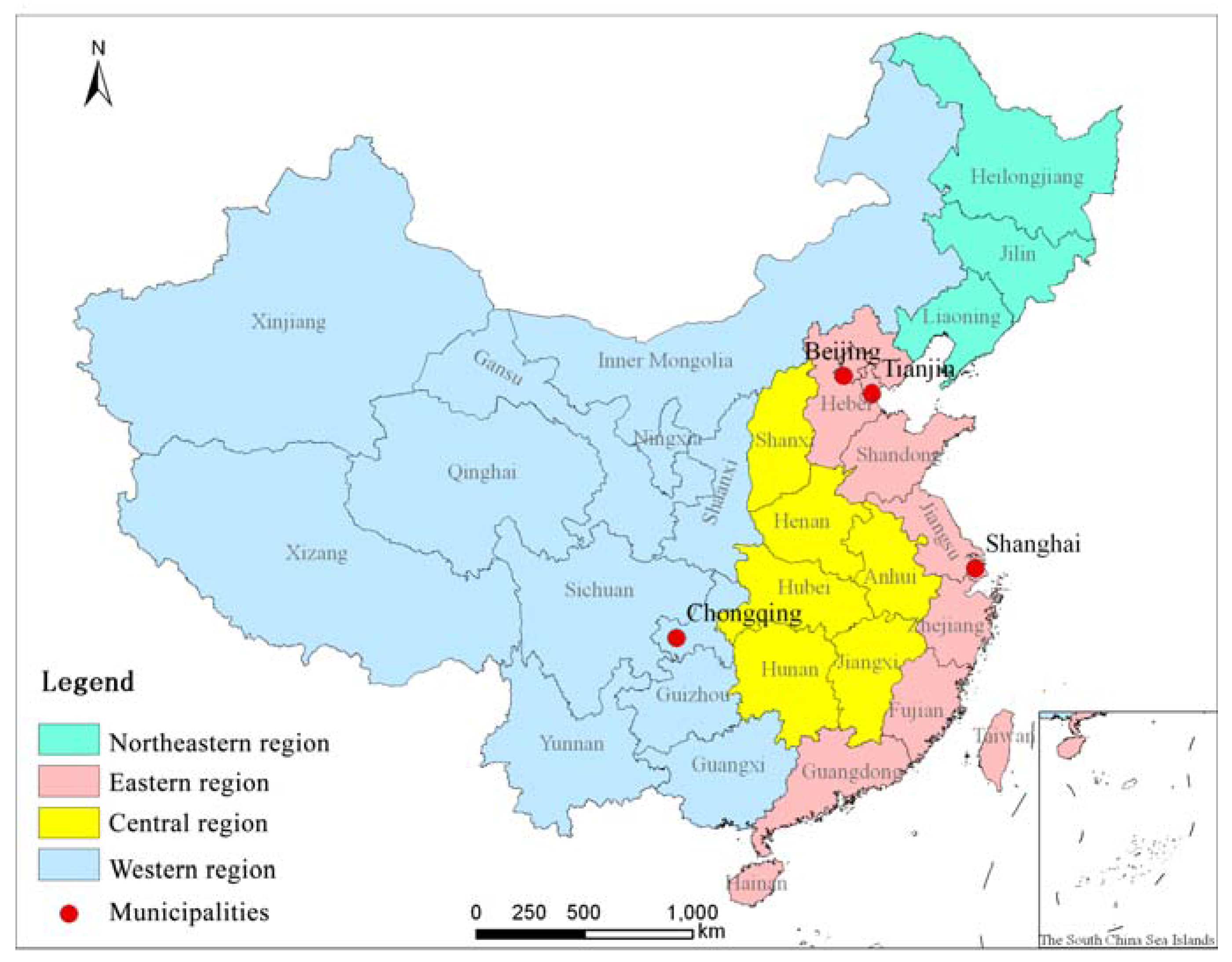
China is the largest developing and most populous country, and lies between 73°33′E–135°05′E and 3°51′N–53°33′N, covering 28 provinces, four municipalities, and two special administrative regions (Figure 1). It is located in the west of the Pacific Ocean and in the east of many Central Asian countries, and has superior conditions of sea and land with convenient traffic and development potentials [49], which promote the development of the economy, culture, and civilization in China and provide good foundations for population growth.
The population distribution of China was obviously different: dense in the east and sparse in the west. According to the latest zoning method proposed by the National Bureau of Statistics of the People’s Republic of China, the Chinese mainland is divided into four economic regions, including the eastern, central, western, and northeastern regions [50,51]. Furthermore, Hong Kong, Macao, and Taiwan are also considered in this work, and are divided into the eastern region.
2.2. Data Source
To obtain a successive and versatile NLT data set, stable light imagery of Version 4 DMSP/OLS NLT products (http://www.ngdc.noaa.gov/eog/dmsp.html) from 1992 to 2013 were employed to calculate the population density in this study, which have a spatial resolution of 30 arc second grids and possess affluent information about the scope and intensity of human activities at night and express lights from cities, towns, and some other persistent lighting sites. The Digital Number (DN) values of these products range from 0 to 63, with high values in the center of urban lands, low values in the peripheral regions, and approximately 0 in uninhabited regions.
Monthly MODIS NDVI (MOD13A3) products (https://modis.gsfc.nasa.gov/) in 2000 and 2010 were used to impair the light saturation and overflowing of NLT products. The former are available from February to December, while the latter can cover every month of the entire year. All these products possess a spatial resolution of 1 km, and cover 1200 columns and 1200 rows. Pre-processing of MOD13A3 NDVI imagery is necessary, and this process mainly includes imagery mosaicking and calculation of the average NDVI. In this work, the former pre-processing step was completed in the MODIS Re-projection Tool software, and the latter was carried out by the function below:
where and are the NDVI values of the th pixel and their average in 2000 or 2010, respectively; j indicates the jth month, and k represents the first month of obtained MOD13A3 NDVI products ( in 2000 and in 2010).
Additionally, Chinese census data in 2000 and 2010 were collected from the National Bureau of Statistics of the People’s Republic of China, and county district-level administrative vector data were obtained from the Data Center for Resources and Environmental Sciences, Chinese Academy of Sciences. To minimize data inconsistency, all remotely-sensed imagery was resampled to the spatial resolution of 1 km in the Asia North Albers Equal Area Conic (AN_Albers) projected coordinate system.
3. Methodology
The methodology of this work mainly includes two parts: (1) correction of NLT products and (2) simulation of population spatialization. The former involves four steps, namely, inter-calibration, geometric, and incompatibility and discontinuity corrections and adjustment based on vegetation information. The latter was accomplished by building the population spatialization simulation model using the corrected NLT products and census data. The main steps of the methodology are summarized in Figure 2.
3.1. Inter-Calibration
Prior to inter-calibration, which was developed by Elvidge et al. [52], the reference image and baseline extents, called the invariant target area, should be defined first. To guarantee high application precision of NLT products, 34 NLT products covering 22 years with sensor-spans of F10 (1992–1994), F12 (1994–1999), F14 (1997–2003), F15 (2000–2007), F16 (2004–2009), and F18 (2010–2013) were employed in this work. The NLT product obtained by the F15 remote sensor in the middle year 2003 was selected as the reference image, and Sicily, Italy was chosen as the invariant target area.
On the basis of the invariant target area, a group of quadratic polynomial regression functions (Equation (2)) were executed between pixel DN values in each candidate NLT product and the reference image, while the corresponding coefficients of determination () (Equation (3)) and mean square error (MSE) (Equation (4)) were generated. By comparison, optimal regression functions of the highest and lowest MSE for inter-calibration were built (Table 1). Then, all coefficients were applied to their corresponding original image products, and the inter-calibrated NLT products were developed:
where and indicate the DN values of the th pixel in the inter-calibrated NLT product and original NLT product; , , and are coefficients; and is the average DN value of all pixels in the original NLT product.
The DN values of pixels in the original NLT products are integers from 0 to 63. In general, 0 and some other low DN values indicate unlit pixels where background noise exists. However, decimals, especially many negative decimals, usually replace the original integers after the inter-calibration step. To obtain reliable light information and DN values, all the DN values smaller than 0 were revalued as 0, and positive DN values were rounded to the nearest integers by adopting Equation (5):
where means the DN values of the th pixel in the inter-calibrated NLT product, and is the DN value of the th pixel after rounding calculation.
3.2. Geometric Correction
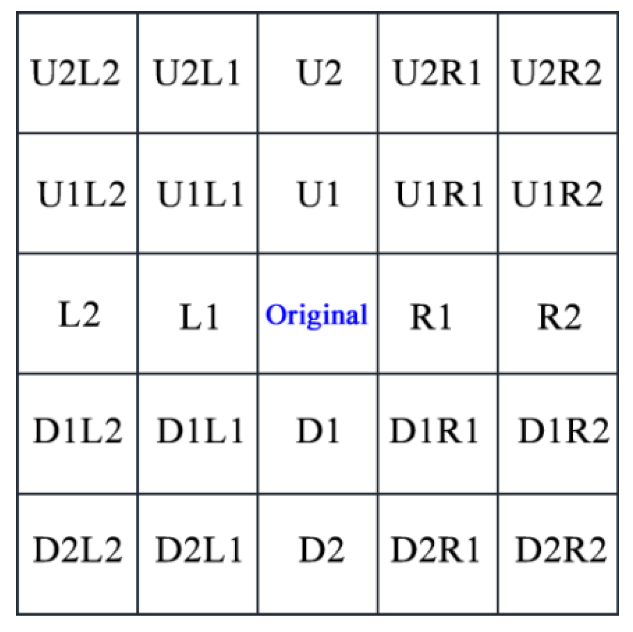
Geometric errors may cause disappearance or regression of some lit pixels. Pixels in NLT products usually generate geometric errors horizontally or vertically from zero to two pixels (Figure 3), mainly including eight directions, namely, up (U), down (D), left (L), right (R), up left (UL), up down (UD), down left (DL), and down right (DR). To eliminate geometric errors, a pixel-based shifting method was employed.
where and represent the column number and the row number of a certain pixel. Equation (6) shows the basic geometric correcting functions for moving one pixel to up, down, left, and right directions, respectively. Geometric correcting to other directions can be executed by the synergistic use of these four functions.
Firstly, F152003 NLT product was selected as the reference image, and each pixel in candidate NLT products was shifted using 25 methods for eight directions. Then, and MSE were calculated by adjusting the pixel DN values in candidate NLT products to match the reference image. Finally, the shift method with the highest and the lowest MSE for each candidate NLT product was selected as its geometric correcting approach (Table 2).
3.3. Incompatibility and Discontinuity Correction
Most NLT products possess a single DN value for each pixel, such as F101992, F101993, and F121995. However, several NLT products in 1994 and from 1997 to 2007 exhibit different DN values for the same pixel. By using incompatibility correcting, the average of two DN values for the same pixel was calculated based on Equation (7), and the two original DN values of this pixel were replaced by the new values:
where is the DN value after the incompatibility correction, represents the th pixel in NLT products, indicates a year which has two NLT products between 1992 and 2013; and are two DN values of NLT products obtained from sensor a and sensor b in the same year.
After incompatibility correction, 22 NLT products of a unique DN value for each pixel in all annual acquisition years from 1992 to 2013 were generated as the compatible datasets. To further improve continuity of the compatible datasets, a bi-directional steady-increase adjustment method was employed [34]. According to Liu et al. [36], light decreases of developing countries should not exist in NLT products. To simplify the experiment, this study assumed that pixels against this principle are abnormal and should be corrected. If the DN values of F101992 NLT product were correct, the DN value of each pixel in a later year should be not smaller than that in the previous year, else a positive-direction adjustment must be executed by employing Equation (8). Meanwhile, if the DN values of F182013 NLT product were right, the DN value of each pixel in an early year should be no larger than that in the later year, otherwise a negative-direction adjustment should be carried out by adopting Equation (9). To efficiently avoid the undersize or oversize of the DN values of pixels, the average of the positive-direction and negative-direction adjustments should be calculated by using Equation (10):
where and are the DN value of the th pixel in after the positive-direction and negative-direction adjustments, respectively. and represent the DN values of the th pixel in the year and . indicates the DN value of the th pixel in the year after the incompatibility and discontinuity correction.
3.4. Adjustment Based on the Vegetation Distribution Information
Zhang et al. [43] proposed the Vegetation Adjusted NLT Urban Index (VANUI) (Equation (11)) based on the stylized fact that vegetation and urban surfaces are inversely correlated and successfully reduced the effects of NLT saturation using VANUI. In this study, MOD13A3 NDVI products and VANUI were applied to eliminate or decrease light overflowing due to their high correlation with population distribution [1,25,44,48]. DN values of NLT products were normalized to the range of [0, 1.0] [44] firstly, and then the adjustment based on the vegetation distribution was accomplished based on Equation (12):
where is the annual mean NDVI derived from MODIS products, is the DN value of the ith pixel in the normalized NLT products.
where is the DN value of the th pixel after the adjustment based on the vegetation distribution information, is the DN value of the th pixel in the year after the incompatibility and discontinuity correction, and indicates the average NDVI value of the th pixel.
3.5. Population Spatialization
Population spatialization is an effective interoperate method that synergistically uses GIS data, remotely-sensed imagery, and census data to obtain detailed population distribution information at different spatial units [53], including administrative levels (i.e., region, province, and county levels) and different pixel-level scales. The basic principle of spatialization is to provide a clear and accurate population to every unit. At present, the most detailed and relatively authoritative population data in China is the census data at county-level scales. Based on this data, we built the regression functions between the population and DN values of the corrected NLT products at county-level scales to map the Chinese population density at a pixel-level in 2000 and 2010.
Firstly, the total population and DN values in the NLT products of each county were calculated. Secondly, in accordance with the relationship between the sum of DN values and census data, the counties were simply divided into part 1 () and part 2 (), and a group of polynomial regression functions between total population and DN values at county-level scales were developed:
where and are the total population and the sum DN values of the th county. and are the regression functions between and . The cubic polynomial regression functions were selected as the optimal functions:
where a, b, and c are optimal coefficients (Table 3).
Table 3 shows that a simple classification of counties leads to higher (0.9062 and 0.6485 in 2000, and 0.7210 and 0.8460 in 2010) than direct use of all counties (0.6272 in 2000 and 0.5131 in 2010).
Thirdly, the cubic polynomial regression function was applied to each pixel to build the initial population distribution maps:
where is the initial population of the th pixel, is the DN value of the th pixel after the adjustment based on the vegetation distribution information.
Fourthly, given the errors from cubic polynomial regression function, the initial population obtained was discrepant to the census data. A proportionality coefficient was built to reduce the errors by:
where is the proportionality coefficient of the th county, is the census data of the th county, is the total initial population of the th county, represents the initial population of the th pixel in the th county.
Finally, the initial population of all pixels was multiplied by the proportionality coefficient of their corresponding counties, and the spatialized population of each pixel was obtained:
where is the spatialized population of the th pixel in the th county.
3.6. Estimation of Corrected NLT Products
The corrected NLT products were evaluated using a comparison of the sum of DN values in acquisition years:
where is the DN value of the ith pixel, k is the total pixel numbers, and is the sum DN values in the year n.
3.7. Population-Weighted Centroid Model
To investigate the temporal change in the population distribution, we employed a population-weighted centroid model [54]:
where and are the abscissa and ordinated of population-weighted centroid in the year , ; is the population of the th pixel in the year , is the total number of pixels, and and denote the abscissa and ordinate of the th pixel.
After determining the location of population centroids in 2000 and 2010, the moving distance D of the centroids are defined below:
where ()
and (,) indicate the abscissa and ordinated of population centroids in and , respectively.
In this work, population-weighted centroids and their moving distances of four economic zones and nine-level population density types in China were calculated.
4. Results and Analysis
4.1. Evaluation of the Corrected NLT Products
The original NLT products presents two drawbacks (Figure 4). One drawback is discontinuous DN values in NLT products across different years. In Figure 4a, the sum of DN values obtained from satellites F10, F12, and F14 increased stably, whereas three abnormal values occurred in F152003, F162005, and F182011 NTL products. The other drawback are incompatible DN values of NLT products in the same year among different individual images, including F10 and F12 in 1994, F12 and F14 from 1997 to 1999, F14 and F15 from 2000 to 2003, and F15 and F16 from 2004 to 2007.
The sum of DN values showed an increasing trend in the periods of 1992–2006 and 2009–2011 after inter-calibration, geometric, and incompatibility corrections. However, two abnormal peak values remained between 2008 and 2012 (Figure 4b). The positive direction adjustment led to larger sums of DN values, whereas the negative-direction adjustment resulted in lower sum DN values. The average of the bi-direction adjustment results was close to the original value, that is, neither enlarged nor largely reduced. Therefore, the synergistic use of inter-calibration and geometric corrections, incompatibility, and discontinuity correction could be applied to obtain consecutive and compatible NLT products.
To further explore the accuracy of the corrected NLT products after the adjustment based on vegetation information, three sample cities (Wuhan, Xi’an, and Urumchi) were selected for normalization and comparison in this work. The saturation and light overflowing of the original NLT products resulted in misjudgment of residential extents, especially overestimation in water areas and peripheral regions (Figure 5). For the entire urban areas, the DN values of the original NTL products were saturated in the urban core and the variations in inner-urban areas were undetectable. For example, the original NLT products showed the entirety of Wuhan, Xi’an, and Urumchi as saturated and only detected the general outline of each city. By contrast, the corrected NLT products presented more similar light information to the radiance calibrated NLT products released by NOAA’s National Centers for Environmental Information (NCEI) and described much detail, in which small county towns were significant with the urban core and the Yangtze River in Wuhan. Moreover, the characteristics of urban sprawl from space were retained in the corrected NLT products. Hence, the corrected NLT products were highly feasible for the following population spatialization.
4.2. Evaluation of the Spatialized Population
The spatialized population in China could be divided into nine types on the basis of the population density classification standard [55,56], namely, core concentration (≥1000 per ), high concentration (500–1000 per ), moderate concentration (400–500 per ), low concentration (200–400 per ), general transition (100–200 per ), relatively sparse (50–100 per ), sparse (25–50 per ), extremely sparse (1–25 per ), and basic no-man (<1 per ) types; these types accounted for 3.00%, 3.66%, 1.91%, 6.66%, 5.89%, 3.60%, 1.64%, 0.68%, and 72.96% of China in 2000, respectively. Compared with census data, the spatialized population clearly described the spatial heterogeneity of the population distribution in detail and presented differences in population density between urban cores and the peripheral regions (Figure 6).
Considering the availability of census data, quantitative tests were performed at national and provincial scales in this study. According to the census data, the total population of China in 2000 and 2010 were 1272.11 million and 1363.62 million, respectively. The total population simulated from the corrected NLT products were 1270.18 million and 1355.91 million in 2000 and 2010, respectively, which were underestimated, resulting from some zero values of the NLT products, but the magnitude and size of their absolute errors (less than 0.80%) were small and could be neglected. Therefore, the spatialized population at national scale was reliable. To verify the accuracy, objectivity, and authenticity of the spatialized population, the spatialized population was evaluated at the provincial level and above by referring to the census data of 28 provinces (Hebei, Shanxi, Inner Mongolia, Liaoning, Jilin, Heilongjiang, Jiangsu, Zhejiang, Anhui, Fujian, Jiangxi, Shandong, Henan, Hubei, Hunan, Guangdong, Guangxi, Hainan, Sichuan, Guizhou, Yunnan, Tibet, Shaanxi, Gansu, Qinghai, Ningxia, Xinjiang, and Taiwan), four municipalities (Beijing, Tianjin, Shanghai, and Chongqing), and two special administrative regions (Hong Kong and Macao). Figure 7 indicates that the spatialized population had a linear correlation with the census data at the provincial level in 2000 and 2010, thereby showing a high accuracy of the spatialized population. Considering the lack of other reference data, especially census data of village-town administrative divisions, no further test was conducted in this work. However, the previous verifications have suggested the feasibility of the proposed correction and population spatialization methodology for NTL products.
4.3. Spatio-Temporal Differences of Estimated Population Distribution and Its Dynamics in Chinese Four Economic Regions
The total population of the estimated results in China increased from 1270.18 million in 2000 to 1355.91 million in 2010 with a slight increase in the average population density from 134 persons per to 143 persons per . Chinese population distributions and dynamics showed obvious regional differences. With the highest urbanization level [57], the eastern region was the most populous with a high population density increasing from 503 persons per in 2000 to 566 persons per in 2010. This region covered 34.33%, 38.65%, 43.53%, 38.11%, 28.19%, 24.60%, 19.20%, 10.16%, and 3.77% of core concentration, high concentration, moderate concentration, low concentration, general transition, relatively sparse, sparse, extremely sparse, and basic no-man types of China, respectively. The central region covered only 10.85% of national territory but reflected 27.12% of the population of China and became the second most populous region with an average population density increasing from 335 persons per in 2000 to 346 persons per in 2010. This region consisted of 28.33% of the core concentration type, 32.97% of the high concentration type, 29.64% of the moderate concentration type, 24.15% of the low concentration type, 15.15% of the general transition type, 10.38% of the relatively sparse type, 8.13% of the sparse type, 4.01% of the extremely sparse type, and 7.56% of the basic no-man type in China. As the old industrial base of China, the northeastern region was the smallest economic region, covering 5.50%, 4.82%, 7.54%, 17.35%, 33.33%, 38.37%, 30.44%, 15.66%, and 6.30% of core concentration, high concentration, moderate concentration, low concentration, general transition, relatively sparse, sparse, extremely sparse and basic no-man types, respectively. This region reflected only 8.15% of the national population. Lower than the national average, the average population density in the northeastern region was only 132 persons per in 2000 and increased to 138 persons per in 2010. The western region included 31.78%, 23.52%, 19.27%, 20.36%, 23.29%, 26.60%, 42.19%, 70.13%, and 82.36% of the core concentration, high concentration, moderate concentration, low concentration, general transition, relatively sparse, sparse, extremely sparse, and basic no-man types, respectively. Although this region was the largest region among the four economic regions, it showed the sparsest average population densities of 52 and 53 persons per in 2000 and 2010, which were far lower than the national averages and increased by only 1 person per in 10 years.
In general, the population-weighted centroid of China moved from the northwest to the southeast direction at a speed of 2.02 km per year from 2000 to 2010 (Table 4). The moving trends of the population-weighted centroids in the eastern, northeastern, and western regions were similar, that is, from the northeast to the southwest. The eastern region presented the most rapidly-moving speed (2.55 km per year), and it was followed by the western (2.32 km per year) and northeastern (0.93 km per year) regions. The moving trend of the population-weighted centroid in the central region was similar to the national trend, that is, from the northwest to the southeast. However, the moving distance in this region was the smallest among all moving distances of the four regions, at a speed of only 0.58 km per year.
4.4. Spatio-Temporal Differences of the Estimated Population Distribution and Its Dynamics among Nine-Level Population Density Types
The population distribution and dynamics among nine-level population density types exhibited significant differences. The core concentration type was the most populous, loading 55.27% population of China with a high average population density of 2587 persons per in 2000 (Figure 8). This type was mainly distributed in core cities with high urbanization levels and active social economic activities, especially in the provincial capitals and above in the Chinese urban agglomerations, such as Beijing in Beijing–Tianjin–Hebei urban agglomeration, Shanghai in the Yangtze River Delta, Chengdu, Chongqing in the Chengdu-Chongqing urban agglomeration, and Guangzhou in the Pearl River Delta. Though the high concentration type was 0.51 times greater than the core concentration type, its population density (685 persons per ) was only a quarter of that in the core concentration type in 2000. The moderate concentration type was the transition type from the high concentration type to the low concentration type, with an average population density of approximately 448 persons per in 2000. The distribution of the high and moderate concentration types was similar, mainly distributing in the relatively-developed regions, especially in the North China Plain. The low concentration type presented an average population density of 293 persons per but possessed the second largest coverage. This type was mainly distributed in the three main plains of China (North China Plain, Northeast China Plain, and Yangtze Plain) and southeast coastal areas. The general transition type mainly aggregated in the Northeast China Plain, Shanxi, the north of Xinjiang, and southeast coastal areas with an average population density of 149 persons per . The relatively sparse, sparse, extremely sparse, and basic no-man types accounted for 82.28% of the national territory, but only reflected 0.97% of the Chinese population in 2000 with low average population densities of 76 persons per , 38 persons per , 14 persons per , and 0, respectively. The relatively sparse type had the similar distribution to the general transition type. The sparse and extremely sparse types mainly scattered in Xinjiang, the north of Heilongjiang, and the central and east regions of Taiwan. Among the nine types, the basic no-man type was the largest with the sparsest population distribution, mainly distributed in Inner Mongolia, Xinjiang, Tibet, the west part of Qinghai, and the central part of Taiwan.
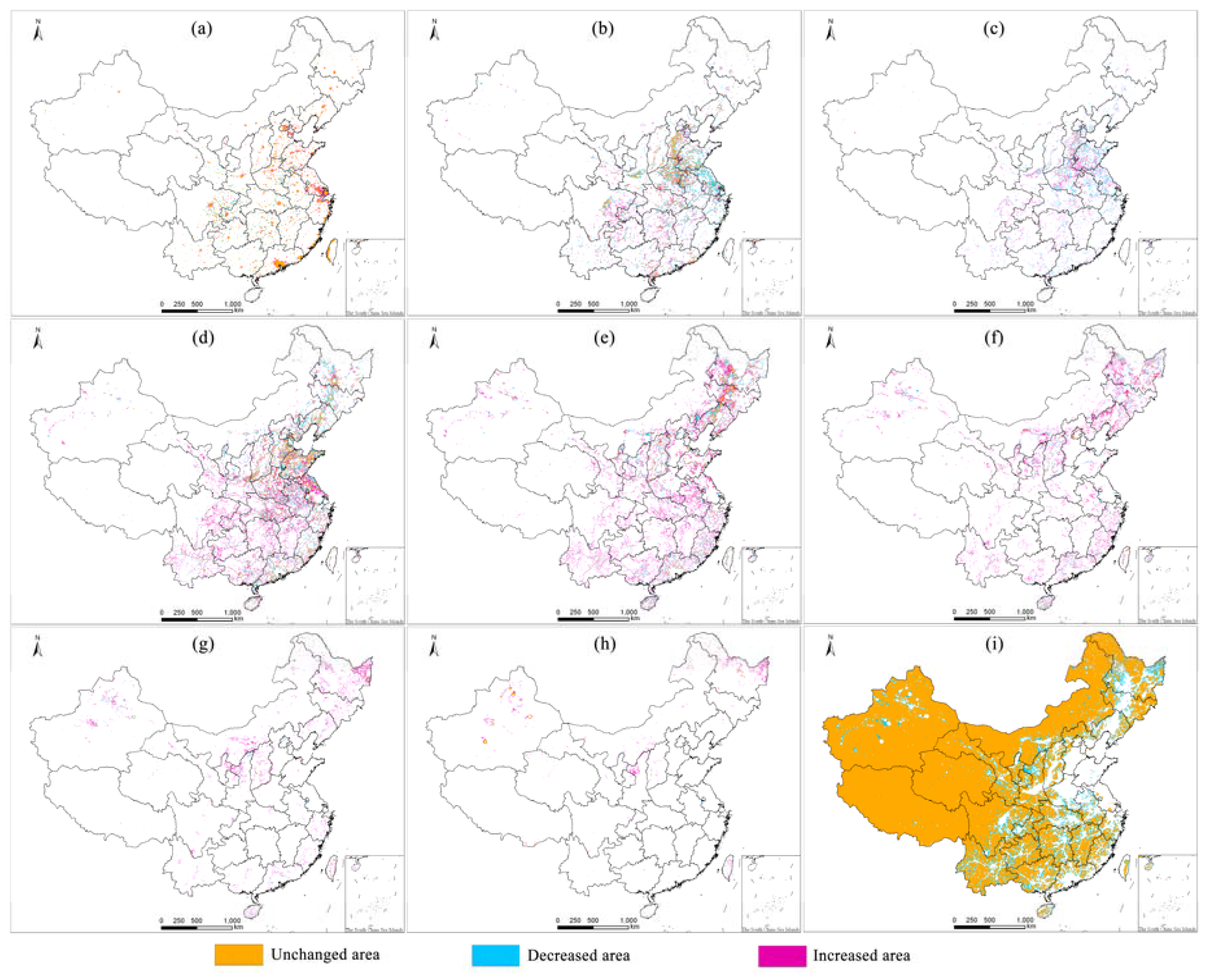
Population distribution among nine-level population density types became wider in 2010 than in 2000 and sprawled from dense areas to sparse areas with amounts of basic no-man-type losses. In general, a net decrease occurred in the high concentration and basic no-man types, whereas a net increase emerged in the seven other types of population density (Figure 6 and Figure 9, and Table 5). The basic no-man type was the sharpest decreasing type with a high net decreased area of 688,688 , which mainly transferred into the relatively sparse, sparse, and extremely sparse types. The second obviously decreasing type was the high concentration type with a net decreased area of 62,739 , which was less than one tenth of that in the basic no-man type and mainly occurred in Shandong and Jiangsu Provinces. The population-weighted centroid of this type moved slightly at a speed of 10.44 km per year from Baitong of Henan Province in 2000 to Zaoyang of Hubei Province along the southwest direction. The first three largest net increase types were the general transition, relatively sparse, and low concentration types, with the net increase at 245,668 , 200,537 and 125,423 , respectively. During 2000–2010, net increase areas of these three types mainly distributed in the eastern, central, and northeastern regions with the population-weighted centroids moving along the southwest direction at a speed of 32.17 km, 33.20 km, and 23.96 km per year, respectively. The net increase in the sparse and extremely sparse types were 118,263 and 49,324 , respectively, which were mainly located in Xinjiang, the middle reach of the Yellow River, and the northeastern region, with the population-weighted centroids moving along the opposite directions at the speed of 20.36 km and 23.60 km per year, respectively. The net increase in the core concentration type was 12,187 , which was only larger than that in the moderate concentration type, and mainly distributed in the edge of core cities of Chinese urban agglomerations, such as peripheral regions of Beijing, Tianjin, and Shijiazhuang in the Beijing–Tianjin–Hebei urban agglomeration, Shanghai, Nanjing, and Hangzhou in the Yangtze River Delta, and Guangzhou, Shenzhen, and Zhuhai in the Pearl River Delta. The population-weighted centroid of the core concentration type transferred along the northeast direction with a moving distance of 110.77 km, only larger than that in the high concentration type. The net increase in the moderate concentration type (25 ) was the least, and mainly appeared in the south of the Shandong Peninsula urban agglomeration with the population-weighted centroid moving 174.42 km along the southwest direction.
In total, population-weighted centroids of the nine population density types mainly distributed in urban agglomerations of the eastern and central regions, of which high-density types are located in the Yangtze River Delta and Central Plains urban agglomeration and low-density types are scattered in the Shandong Peninsula urban agglomeration, Beijing–Tianjin–Hebei urban agglomeration, and Huhhot–Baotou–Ordos–Yulin urban agglomeration. Notably, high population density meant short moving distance of the population-weighted centroid.
5. Discussion
This work was an attempt to reveal the spatio-temporal characteristics of population distribution and dynamics using corrected NLT products. Although previous studies [1,30,46,47,48] have explored various correcting methods of NLT products and have shown the feasibility of NLT products on population simulation, studies in synergistic application of systematic correction of NLT products and population spatialization are scarce. Though case studies on population spatialization with high accuracy existed, they concentrated mainly on early years before 2000 and used complicated steps [1,30,32,48]. Furthermore, detailed analysis on the evolution of spatio-temporal characteristics of the Chinese population is relatively lacking. In this work, these three issues are all solved.
Under powerful guidance of policies, such as the planning of the coastal economic belt development proposed in 2009, the eastern region presented the most rapidly-moving speed of the population-weighted centroid and the strongest attraction for the population with a relatively flat terrain, convenient transportation by sea and land, and a developed economy, which was also supported by Yu et al. [58] and Shi et al. [51]. The central region, which is the second most developed economic region, exhibits congenital advantages in population growth with rich natural resources, convenient land transportation, relatively developed economy, and abundant agriculture and modern industry. According to Wang et al. [59], the population increase and the slowest movement of the population-weighted centroid along the southeast direction in the central region were influenced by the improvement of residents’ income and living standards. The northeastern region is located in the core area of East Asia. The region exhibits great reclamation potential with abundant black soil, but its population is less than that in the eastern and central regions as a result of its relatively high latitude and low temperature, and presented a movement of the population-weighted centroid along the southwest direction, which was consistent with the movement of socio-economic and land urbanization proposed by Gan et al. [60]. The results showed a constantly-improved coupling relationship between the population and land urbanization in the northeastern region, which supported the standpoint of Guo et al. [61]. Compared with the three other regions, the western region is undeveloped and possesses relatively weak advantages for population growth owing to its inconvenient transportation and special climate environment, which was consistent with Qian et al. [62]. In the present work, the obviously different natural and social-economic characteristics of the four regions resulted in significant regional differences of population distribution and evolution. The eastern region presented the densest population and the largest population density increase, and it was followed by the central and northeastern regions, and the western region with the smallest population density, which was consistent with the results of Zhuo et al. [32] and Zeng et al. [1].
Although corrected NLT products were successfully used for population spatialization of China in 2000 and 2010, two limitations still existed. (1) In accordance with Zhang et al. [43], the adjustment based on vegetation information was completed and impaired light overflowing to some extent. However, the adjustment was still limited and needs to be further improved because of its unobvious effect in core areas of cities. This finding coincided with the results of Li [63] and Ni [64]. (2) Zero population density could not reflect the actuality in some places, such as some lagged villages with relatively unpopular electricity. To address these limitations, spatial interpolation, geographical factor fitting, and other new approaches should be considered in further studies.
6. Conclusions
In this study, 34 obtained NLT products were corrected and the corrected NLT products were then applied to the subsequent population spatialization. The conclusions obtained are as follows:
(1) The inter-calibration, geometric, and incompatibility and discontinuity corrections successfully eliminated abnormal and incompatible DN values in the original NLT products. The adjustment based on vegetation information efficiently impaired saturation and light overflowing to some extent, especially in the peripheral regions.
(2) The population spatialization method was easy to execute and available for the subsequent analysis on population distribution and evolution in China. During verification using limited reference data, the spatialized population distribution maps presented low relative errors with less than 0.80% at the national scale and robust linear correlation at the provincial scale.
(3) The spatio-temporal characteristics of population distribution and evolution exhibited obvious regional differences in the four economic regions. Among the four regions, the eastern region possessed the densest population, the quickest population density increase, and the most rapidly-moving speed of the population-weighted centroid along the southwest direction. The central region exhibited the second densest population, the second quickest population density increase, and the slowest moving speed of the population-weighted centroid along the southeast direction. The northeastern region presented the third most rapidly-moving speed of the population-weighted centroid along the southwest direction. The western region showed the sparsest population, the slightest population density increase, and the second most rapidly-moving speed of population-weighted centroid along the southwest direction.
(4) The population distribution and dynamics among the nine-level population density types exhibited significant differences. The high-density types showed a dense population and slow moving speed of the population-weighted centroids. By contrast, the low-density types exhibited sparse population and rapid moving speed of the population-weighted centroids. The population dynamics and moving direction of the population-weighted centroids exhibited apparent differences with a net decrease occurring in high concentration and basic no-man types. A net increase emerged in the seven other population density types. Population-weighted centroids moved along the northeast direction for the core concentration and extremely sparse types, whereas they moved along the southwest direction for the seven other types.
In summary, the application of the corrected NLT products is an effective method to spatialize the population to grid units of 1 km × 1 km and exhibit the spatial heterogeneity of the population distribution in detail. As the important databases of Chinese population, the estimated results are available for recognizing population density, formulating reasonable population planning as a reference, and providing scientific accordance for other corresponding studies and strategies in China. In addition, by the synergistic use of the estimated results and feasible prediction models, the trend of population increase and dynamics in the future periods should become available.
Acknowledgments
This research was supported by National Key Research and Development Plan, ‘Dynamic monitoring and evaluation of gully erosion in black soil region Northeast China’ (Grant No. 2017YFC0504201) and the International Partnership Program of Chinese Academy of Sciences (Grant No. 131C11KYSB20160061).
Author Contributions
Sisi Yu conceived and designed the experiments and processed the data. Based on the processed data, Sisi Yu and Fang Liu analyzed the data and drafted the initial manuscript. Fang Liu and Zengxiang Zhang reviewed and commented on the manuscript.
Conflicts of Interest
The authors declare no conflict of interest.
References
- Zeng, C.; Zhou, Y.; Wang, S.; Yan, F.; Zhao, Q. Population spatialization in China based on night-time imagery and land use data. Int. J. Remote Sens. 2011, 24, 9599–9620. [Google Scholar] [CrossRef]
- Obienusi, E.A.; Ekezie, M.; Onwuka, S.U. Investigating the place of population increase and level of income earning in food security a study of yam supply in Awka urban, Anambra state of Nigeria. J. Nat. Sci. Res. 2014, 11, 11–21. [Google Scholar]
- Hutchinson, J.; Hutchinson, J. Population and food supply. BMJ-Br. Med. J. 1969, 3893, 320. [Google Scholar]
- Wang, C.; Liu, Y.; Kong, X.; Li, J. Spatiotemporal decoupling between population and construction land in urban and rural Hubei province. Sustainability 2017, 7, 1258. [Google Scholar] [CrossRef]
- Zhang, Y. Research on the effects of changes in the age structure of China’s population to energy consumption: Based on the provincial dynamic panel data by GMM. China Popul. Resour. Environ. 2015, 11, 69–74. [Google Scholar]
- Yigzaw, W.; Hossain, F. Water sustainability of large cities in the United States from the perspectives of population increase, anthropogenic activities, and climate change. Earths Future 2016, 12, 603–617. [Google Scholar] [CrossRef]
- Atasoylu, G.; Evci, E.D.; Kaya, E.; Ergin, F.; Tikir, D.; Beser, E. The household garbage in the western coast region of Turkey and its relationship with the socio-economic characteristics. J. Environ. Biol. 2007, 28, 225–229. [Google Scholar] [PubMed]
- János, N. Climate change, agricultural land use and food safety. Econ. Aic 2014, 7, 149–157. [Google Scholar]
- Li, L.; Lei, Y.; Pan, D.; Si, C. Research on sustainable development of resource-based cities based on the DEA approach: A case study of Jiaozuo, China. Math. Probl. Eng. 2016, 3, 1–10. [Google Scholar] [CrossRef]
- Miao, C.L.; Sun, L.Y.; Yang, L. The studies of ecological environmental quality assessment in Anhui Province based on ecological footprint. Ecol. Indic. 2016, 60, 879–883. [Google Scholar] [CrossRef]
- Pan, R.; Liu, Y.; Sun, H. The coupling analysis of population urbanization and economic development: Take the case of counties (Cities, Areas) of Henan Province. Geomat. Spat. Inf. Technol. 2016, 3, 85–89. [Google Scholar]
- Ma, T.; Zhou, Y.; Zhou, C.; Haynie, S.; Pei, T.; Xu, T. Night-time light derived estimation of spatio-temporal characteristics of urbanization dynamics using DMSP/OLS satellite data. Remote Sens. Environ. 2015, 158, 453–464. [Google Scholar] [CrossRef]
- Bennett, M.M.; Smith, L.C. Advances in using multitemporal night-time lights satellite imagery to detect, estimate, and monitor socioeconomic dynamics. Remote Sens. Environ. 2017, 192, 176–197. [Google Scholar] [CrossRef]
- Proville, J.; Zavalaaraiza, D.; Wagner, G. Night-time lights: A global, long term look at links to socio-economic trends. PLoS ONE 2017, 3, e0174610. [Google Scholar] [CrossRef] [PubMed]
- Gao, Q.; Ka-Simu, A. Modeling the population spatial distribution of Tianshan north-slope urban agglomeration based on DMSP/OLS night lighting data. Northwest Popul. J. 2017, 3, 113–120. [Google Scholar]
- Letu, H.; Hara, M.; Tana, G.; Bao, Y.; Nishio, F. Generating the nighttime light of the human settlements by identifying periodic components from DMSP/OLS satellite imagery. Environ. Sci. Technol. 2015, 17, 10503–10509. [Google Scholar] [CrossRef] [PubMed]
- Amaral, S.; Câmara, G.; Monteiro, A.M.V.; Quintanilha, J.A.; Elvidge, C.D. Estimating population and energy consumption in Brazilian Amazonia using DMSP night-time satellite data. Comput. Environ. Urban Syst. 2005, 2, 179–195. [Google Scholar] [CrossRef]
- Xie, Y.; Weng, Q. World energy consumption pattern as revealed by DMSP-OLS nighttime light imagery. Gisci. Remote Sens. 2016, 2, 265–282. [Google Scholar] [CrossRef]
- Wang, Y.; Li, G. Mapping urban CO2 emissions using DMSP/OLS’ city lights satellite data in China. Environ. Plan. A 2017, 2, 248–251. [Google Scholar] [CrossRef]
- Shi, K.; Chen, Y.; Yu, B.; Xu, T.; Chen, Z.; Liu, R.; Li, L.; Wu, J. Modeling spatiotemporal CO2 (carbon dioxide) emission dynamics in China from DMSP-OLS nighttime stable light data using panel data analysis. Appl. Energy 2016, 168, 523–533. [Google Scholar] [CrossRef]
- Guo, X.; Yan, Q.; Tan, X.; Liu, S. Spatial distribution of carbon emissions based on DMSP/OLS nighttime light data and NDVI in Jiangsu province. World Reg. Stud. 2016, 4, 102–110. [Google Scholar]
- Letu, H.; Takashi, Y.N.; Fumihiko, N. Regional-scale estimation of electric power and power plant CO2 emissions using defense meteorological satellite program operational linescan system nighttime satellite data. Environ. Sci. Technol. Lett. 2014, 1, 259–265. [Google Scholar] [CrossRef]
- Jiang, W.; He, G.; Long, T.; Wang, C.; Ni, Y.; Ma, R. Assessing Light Pollution in China Based on Nighttime Light Imagery. Remote Sens. 2017, 2, 135. [Google Scholar] [CrossRef]
- Guo, S.; Gong, J.; Yin, J. Study on grid refinement for population distribution based on DMSP/OLS. J. Seismol. Res. 2016, 2, 321–326. [Google Scholar]
- Song, G.; Yu, M.; Liu, S.; Zhang, S. A dynamic model for population mapping: A methodology integrating a Monte Carlo simulation with vegetation-adjusted night-time light images. Int. J. Remote Sens. 2015, 15, 4055–4068. [Google Scholar] [CrossRef]
- Huang, J.; Yan, Q.; Liu, Y. Modeling the population density of Jiangsu Province based on DMSP/OLS satellite imagery and land use data. Resour. Environ. Yangtze Basin 2015, 5, 735–741. [Google Scholar]
- Yang, X.; Yue, W.; Gao, D. Spatial improvement of human population distribution based on multi-sensor remote-sensing data: An input for exposure assessment. Int. J. Remote Sens. 2013, 15, 5569–5583. [Google Scholar] [CrossRef]
- Shao, Z.; Liu, C. The integrated use of DMSP-OLS Nighttime Light and MODIS data for monitoring large-scale impervious surface dynamics: A case study in the Yangtze River Delta. Remote Sens. 2014, 6, 9359–9378. [Google Scholar] [CrossRef]
- Bai, Z.; Wang, J. Generation of high resolution population distribution map in 2000 and 2010: A case study in the Loess Plateau, China. In Proceedings of the International Conference on Geoinformatics, Wuhan, China, 19–21 June 2015; pp. 1–6. [Google Scholar]
- Lo, C.P. Modeling the population of china using DMSP operational linescan system nighttime data. Photogramm. Eng. Remote Sens. 2001, 9, 1037–1047. [Google Scholar]
- Geer, S.D. A map of the distribution of population in Sweden: Method of preparation and general results. Geogr. Rev. 1922, 1, 72–83. [Google Scholar] [CrossRef]
- Zhuo, L.; Ichinose, T.; Zheng, J.; Chen, J.; Shi, P.; Li, X. Modelling the population density of China at the pixel level based on DMSP/OLS non-radiance-calibrated night-time light images. Int. J. Remote Sens. 2009, 4, 1003–1018. [Google Scholar] [CrossRef]
- Illeris, S. Counter-urbanization revisited: The new map of population distribution in central and north-western Europe. Nor. Geogr. Tidsskr. 1990, 1, 39–52. [Google Scholar] [CrossRef] [PubMed]
- Zhao, N.; Zhou, Y.; Samson, E.L. Correcting incompatible DN values and geometric errors in nighttime lights time-series images. IEEE Trans. Geosci. Remote Sens. 2015, 4, 2039–2049. [Google Scholar] [CrossRef]
- Zhao, N.; Ghosh, T.; Samson, E.L. Mapping spatio-temporal changes of Chinese electric power consumption using night-time imagery. Int. J. Remote Sens. 2012, 20, 6304–6320. [Google Scholar] [CrossRef]
- Liu, Z.; He, C.; Zhang, Q.; Huang, Q.; Yang, Y. Extracting the dynamics of urban expansion in China using DMSP-OLS nighttime light data from 1992 to 2008. Landsc. Urban Plan. 2012, 1, 62–72. [Google Scholar] [CrossRef]
- Cao, Z.; Wu, Z.; Kuang, Y.; Huang, N. Correction of DMSP/OLS night-time light images and its application in China. J. Geo-Inf. Sci. 2015, 1, 1010–1016. [Google Scholar]
- Letu, H.; Hara, M.; Yagi, H.; Tana, G. Estimating the energy consumption with nighttime city light from the DMSP/OLS imagery. In Proceedings of the Urban Remote Sensing Event, Shanghai, China, 20–22 May 2009; pp. 1–7. [Google Scholar]
- Letu, H.; Hara, M.; Tana, G.; Nishio, F. A saturated light correction method for DMSP/OLS nighttime satellite imagery. IEEE Trans. Geosci. Remote Sens. 2012, 2, 389–396. [Google Scholar] [CrossRef]
- Raupach, M.; Rayner, P.; Paget, M. Regional variations in spatial structure of nightlights, population density and fossil-fuel CO2 emissions. Energy Policy 2010, 9, 4756–4764. [Google Scholar] [CrossRef]
- Wu, J.; He, S.; Peng, J.; Li, W.; Zhong, X. Intercalibration of DMSP-OLS night-time light data by the invariant region method. Int. J. Remote Sens. 2013, 20, 7356–7368. [Google Scholar] [CrossRef]
- Hsu, F.C.; Baugh, K.E.; Ghosh, T.; Zhizhin, M.; Elvidge, C.D. DMSP-OLS radiance calibrated nighttime lights time series with intercalibration. Remote Sens. 2015, 2, 1855–1876. [Google Scholar] [CrossRef]
- Zhang, Q.; Schaaf, C.; Seto, K.C. The vegetation adjusted NTL urban index: A new approach to reduce saturation and increase variation in nighttime luminosity. Remote Sens. Environ. 2013, 2, 32–41. [Google Scholar] [CrossRef]
- Zhuo, L.; Zhang, X.; Zheng, J.; Tao, H.; Guo, Y. An EVI-based method to reduce saturation of DMSP/OLS nighttime light data. Acta Geogr. Sin. 2015, 8, 1339–1350. [Google Scholar]
- Cao, L.; Li, P.; Zhang, L. Urban population estimation based on the DMSP/OLS night-time satellite data——A case of Hubei Province. Remote Sens. Inf. 2009, 4, 35–45. [Google Scholar]
- Li, P.; Hong, H. Estimation of urban population in Guangdong Province based on DMSP-OLS lighting data. J. South China Normal Univ. (Nat. Sci. Ed.) 2015, 2, 102–107. [Google Scholar]
- Liang, Y.; Xu, Z. Modeling the spatial distribution of GDP based on night light radiation: A case study in Ganzhou District, Zhangye Municipality. J. Glaciol. Geocryol. 2013, 1, 249–254. [Google Scholar]
- Zhuo, L.; Chen, J.; Shi, P.; Gu, Z.; Fan, Y.; Yi, Z. Modeling population density of china in 1998 based on DMSP/OLS nighttime light image. Acta Geogr. Sin. 2005, 2, 266–276. [Google Scholar]
- Gu, X.; Li, M.; Xu, D.; Zhang, B.; Nie, X.; Li, H.; Wang, S.; Zhang, Z.; Liu, Q.; Li, J. Report on Remote Sensing Monitoring of China Sustainable Development (2016); Social Sciences Academic Press: Beijing, China, 2016. [Google Scholar]
- Hou, X. Research on the balanced development of China’s urbanization and industrialization in eastern, central, western and northeastern regions. Asian Agric. Res. 2011, 3, 124–128. [Google Scholar]
- Shi, L.; Taubenböck, H.; Zhang, Z.; Liu, F.; Wurm, M. Urbanization in China from the end of 1980s until 2010—Spatial dynamics and patterns of growth using EO-data. Int. J. Digit. Earth 2017, 1–17. [Google Scholar] [CrossRef]
- Elvidge, C.D.; Ziskin, D.; Baugh, K.E.; Tuttle, B.T.; Ghosh, T.; Pack, D.W.; Erwin, E.H.; Zhizhin, M. A Fifteen Year Record of Global Natural Gas Flaring Derived from Satellite Data. Energies 2009, 3, 595–622. [Google Scholar] [CrossRef]
- Bo, Z.; Wang, J.; Yang, F. Research progress in spatialization of population data. Prog. Geogr. 2013, 11, 1692–1702. [Google Scholar]
- Wang, S.; Liu, J.; Zhang, Z.; Zhou, Q.; Wang, C. Spatial pattern change of land use in china in recent 10 years. Acta Geogr. Sin. 2002, 5, 523–530. [Google Scholar]
- Ge, M.; Feng, Z. Population distribution of china based on GIS: Classification of population densities and curve of population gravity centers. Acta Geogr. Sin. 2009, 2, 202–210. [Google Scholar]
- Yang, Q.; Li, L.; Wang, Y.; Wang, X.; Lu, Y. Spatial distribution pattern of population and characteristics of its evolution in China during 1935–2010. Geogr. Res. 2016, 8, 1547–1560. [Google Scholar]
- Fan, J.; Liu, J.; Zhang, X.; Cumtb, B. Urbanization Effect on Regional Household Energy Consumption in China. China Popul. Resour. Environ. 2015, 1, 55–60. [Google Scholar]
- Xiao, Y.; Li, Y.; Lei, J. Analysis on China’s Provincial Population Migration and Its Impact on Regional Economic Development since the New Century. Popul. J. 2013, 3, 5–14. [Google Scholar]
- Wang, G. Migration and Regional Development in Central China: Evidence based on Fifth Census and Sixth Census. Econ. Probl. 2017, 5, 123–129. [Google Scholar]
- Gan, J.; Guo, F.; Chen, C.; Liu, J.; Li, Z. The Spatio-temporal Evolution Characteristics of Urbanization Spatial Differentiation in Northeast China. Sci. Geogr. Sin. 2015, 5, 565–574. [Google Scholar]
- Guo, F.; Gu, L.; Chen, C.; Gan, J. Spatial-Temporal Coupling Characteristics of Population Urbanization and Land Urbanization in Northeast China. Econ. Geogr. 2015, 9, 49–56. [Google Scholar]
- Qian, S. Research on population growth of large cities in Central and Western regions. Spec. Zone Econ. 2007, 9, 159–161. [Google Scholar]
- Li, Q.; Lu, L.; Weng, Q.; Xie, Y.; Guo, H. Monitoring urban dynamics in the southeast U.S.A. using time-series DMSP/OLS nightlight imagery. Remote Sens. 2016, 7, 578. [Google Scholar] [CrossRef]
- Ni, Y.; Zhou, X.; Jiang, W. A reducing saturation method for DMSP/OLS nighttime light image combining Landsat data. Remote Sens. Technol. Appl. 2017, 4, 721–727. [Google Scholar]
Figure 1.
Study area distribution.

Figure 2.
Flowchart for generating the spatialized population map using nighttime lights time-series (NLT) data.
Figure 2.
Flowchart for generating the spatialized population map using nighttime lights time-series (NLT) data.
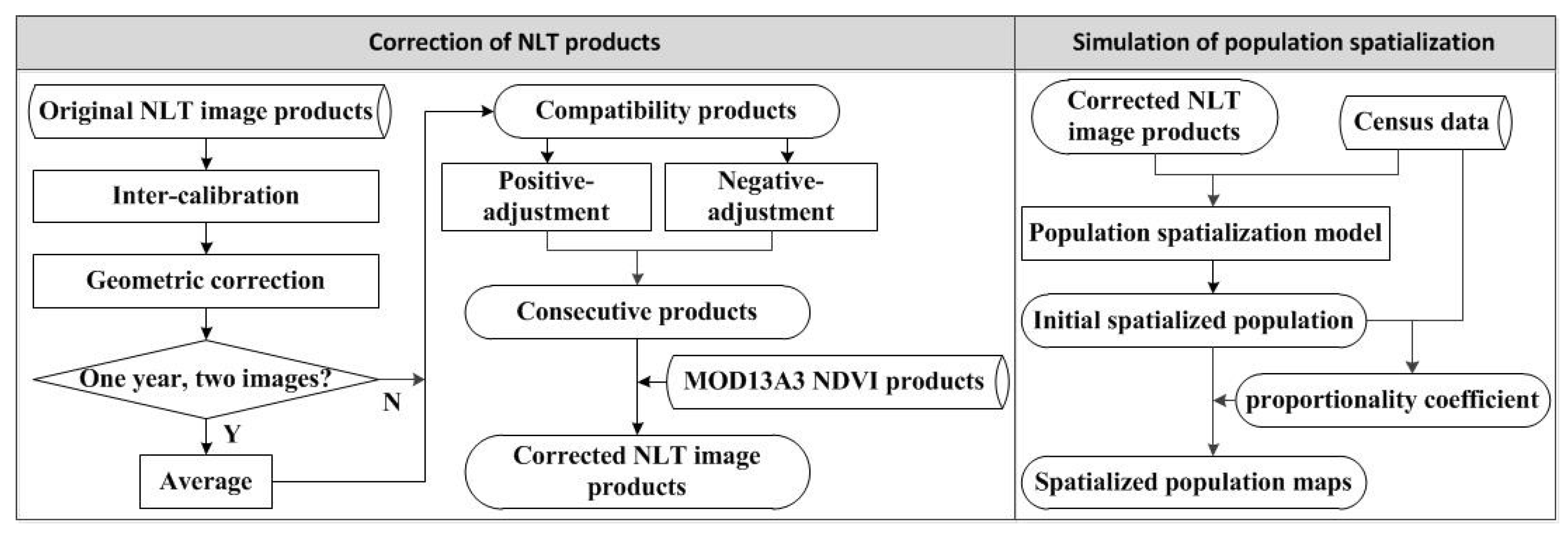
Figure 3.
Geographic deviation directions.

Figure 4.
The sum of Digital Number (DN) values of the (a) original and (b) corrected NLT products in China.
Figure 4.
The sum of Digital Number (DN) values of the (a) original and (b) corrected NLT products in China.
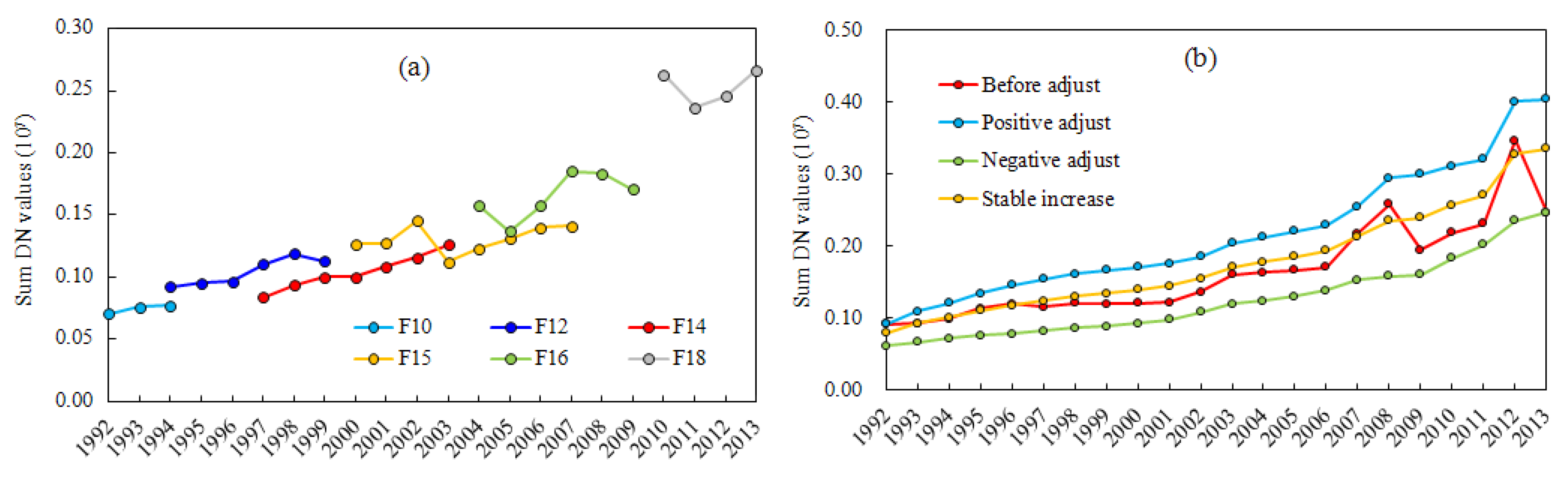
Figure 5.
Normalized NLT products before and after adjustment based on vegetation information for selected cities.
Figure 5.
Normalized NLT products before and after adjustment based on vegetation information for selected cities.
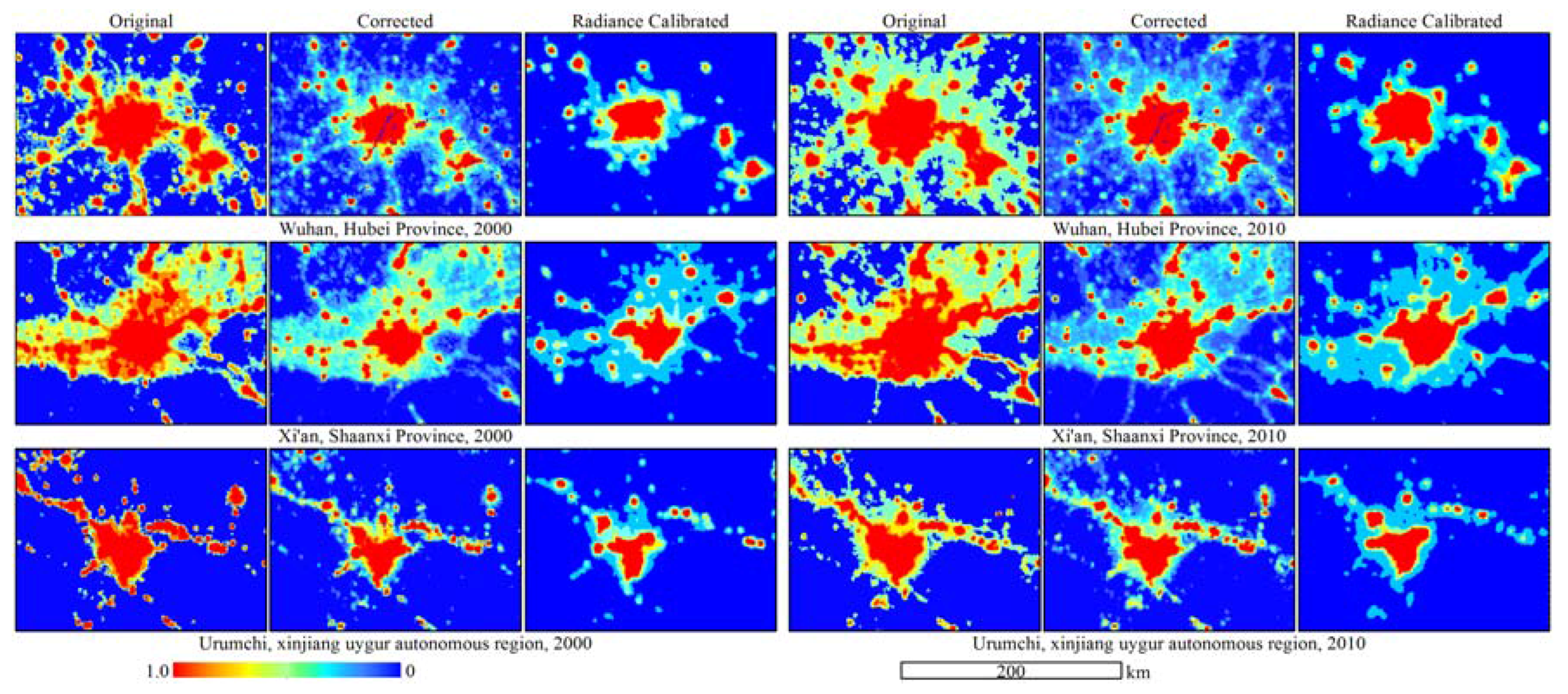
Figure 6.
Simulated population density (per ) spatialized for China in (a) 2000 and (b) 2010.
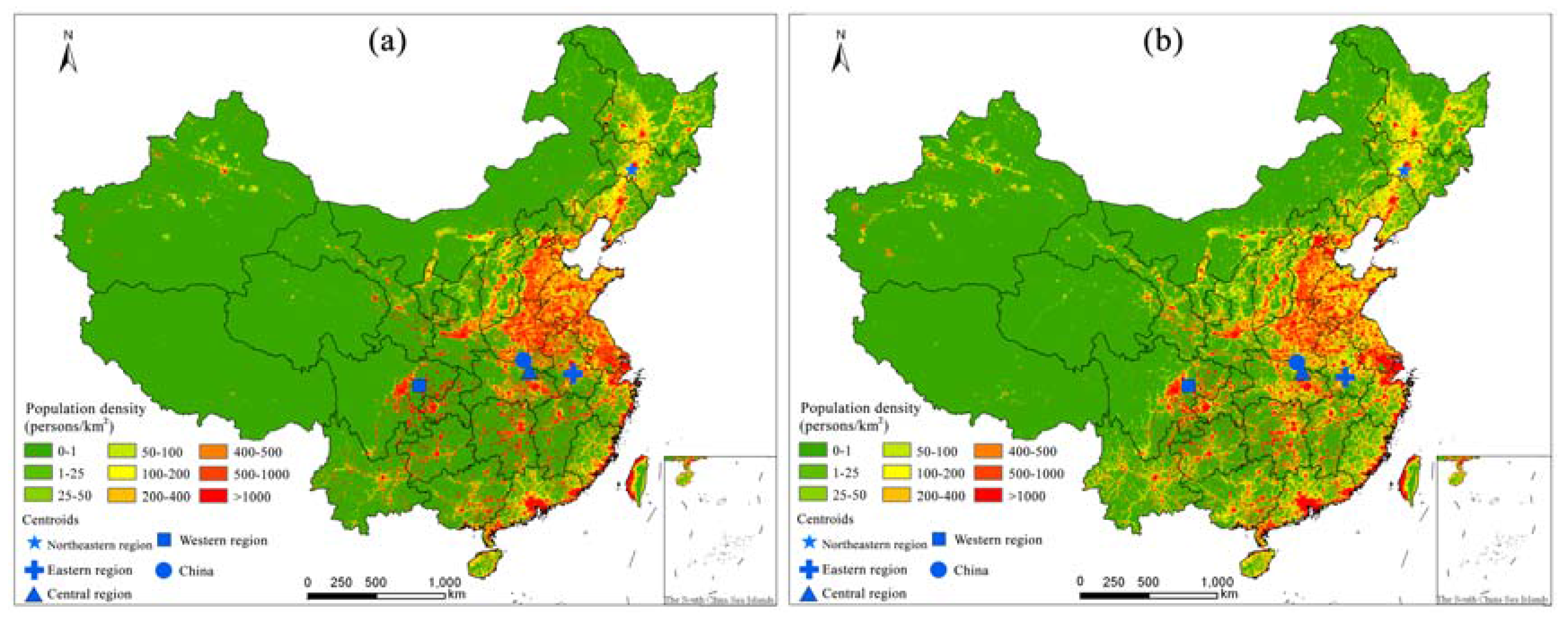
Figure 7.
Relationships between the census data and the spatialized population at the provincial level in (a) 2000 and (b) 2010.
Figure 7.
Relationships between the census data and the spatialized population at the provincial level in (a) 2000 and (b) 2010.
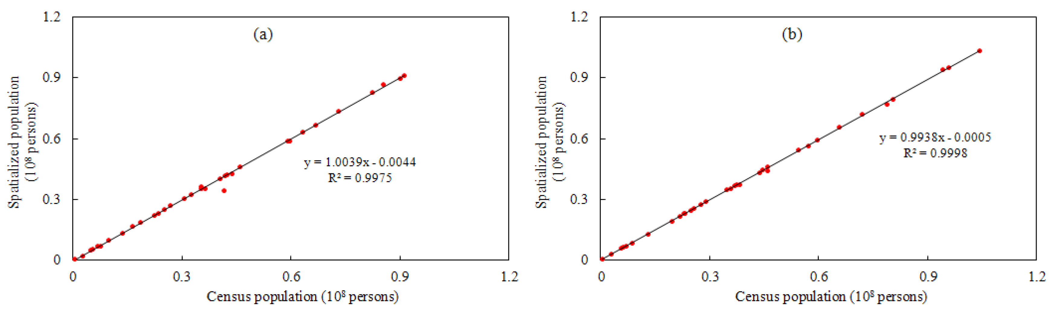
Figure 8.
Population distribution of nine-level types in 2000, including (a) core concentration, (b) high concentration, (c) moderate concentration, (d) low concentration, (e) general transition, (f) relatively sparse, (g) sparse, (h) extremely sparse, and (i) basic no-man types.
Figure 8.
Population distribution of nine-level types in 2000, including (a) core concentration, (b) high concentration, (c) moderate concentration, (d) low concentration, (e) general transition, (f) relatively sparse, (g) sparse, (h) extremely sparse, and (i) basic no-man types.
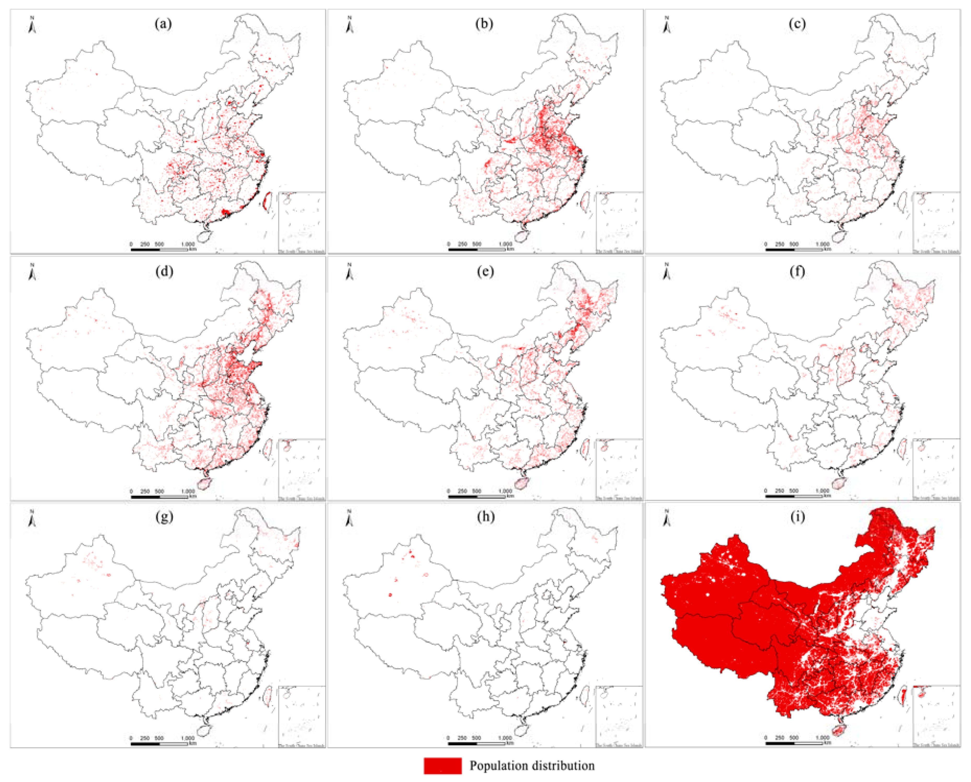
Figure 9.
Population distribution evolution of nine-level types in 2000–2010, including (a) core concentration, (b) high concentration, (c) moderate concentration, (d) low concentration, (e) general transition, (f) relatively sparse, (g) sparse, (h) extremely sparse, and (i) basic no-man types.
Figure 9.
Population distribution evolution of nine-level types in 2000–2010, including (a) core concentration, (b) high concentration, (c) moderate concentration, (d) low concentration, (e) general transition, (f) relatively sparse, (g) sparse, (h) extremely sparse, and (i) basic no-man types.

Table 1.
Regression function for inter-calibration of NLT products.
| Satellite | α0 | α1 | α2 | R2 | MSE |
|---|---|---|---|---|---|
| F101992 | 0.9977 | 0.8210 | 0.0020 | 0.9322 | 4.4541 |
| F101993 | −0.3270 | 1.0045 | −0.0005 | 0.9655 | 3.1623 |
| F101994 | 1.0659 | 0.8465 | 0.0013 | 0.9603 | 3.3984 |
| F121994 | 1.5212 | 0.5684 | 0.0058 | 0.9611 | 3.3650 |
| F121995 | 0.8347 | 0.6920 | 0.0036 | 0.9642 | 3.2285 |
| F121996 | 1.3949 | 0.6709 | 0.0045 | 0.9667 | 3.1131 |
| F121997 | 0.8742 | 0.6295 | 0.0050 | 0.9654 | 3.1744 |
| F121998 | 1.0554 | 0.5449 | 0.0055 | 0.9736 | 2.7661 |
| F121999 | 1.5706 | 0.4731 | 0.0063 | 0.9613 | 3.3543 |
| F141997 | 0.1358 | 1.0701 | −0.0011 | 0.9656 | 3.1639 |
| F141998 | 1.0393 | 0.9663 | −0.0005 | 0.9618 | 3.3234 |
| F141999 | 0.4384 | 0.9250 | 0.0004 | 0.9632 | 3.2734 |
| F142000 | 1.2695 | 0.8043 | 0.0018 | 0.9569 | 3.5542 |
| F142001 | 0.7832 | 0.7858 | 0.0023 | 0.9654 | 3.1642 |
| F142002 | 1.3648 | 0.6628 | 0.0040 | 0.9821 | 2.2809 |
| F142003 | 0.7706 | 0.7699 | 0.0025 | 0.9680 | 3.0499 |
| F152000 | 0.4816 | 0.5850 | 0.0051 | 0.9780 | 2.5347 |
| F152001 | 0.5699 | 0.5790 | 0.0058 | 0.9806 | 2.3729 |
| F152002 | 1.1773 | 0.4723 | 0.0070 | 0.9774 | 2.5632 |
| F152004 | 1.2652 | 0.7661 | 0.0030 | 0.9784 | 2.5022 |
| F152005 | 0.5865 | 0.7904 | 0.0029 | 0.9830 | 2.2167 |
| F152006 | 0.8930 | 0.7697 | 0.0033 | 0.9798 | 2.4200 |
| F152007 | 1.5459 | 0.7567 | 0.0035 | 0.9580 | 3.4947 |
| F162004 | 0.9376 | 0.6658 | 0.0042 | 0.9838 | 2.1760 |
| F162005 | 0.2044 | 0.8927 | 0.0010 | 0.9649 | 3.1913 |
| F162006 | 1.1505 | 0.6044 | 0.0056 | 0.9583 | 3.4863 |
| F162007 | 1.3989 | 0.4562 | 0.0069 | 0.9664 | 3.1223 |
| F162008 | 1.2588 | 0.5202 | 0.0059 | 0.9686 | 3.0233 |
| F162009 | 1.8401 | 0.5536 | 0.0054 | 0.9616 | 3.3361 |
| F182010 | 2.1357 | 0.1869 | 0.0104 | 0.9628 | 3.2883 |
| F182011 | 2.2331 | 0.3531 | 0.0072 | 0.9228 | 4.7330 |
| F182012 | 2.0651 | 0.2699 | 0.0088 | 0.9524 | 3.7276 |
| F182013 | 1.9631 | 0.3237 | 0.0077 | 0.9631 | 3.2806 |
Table 2.
Movement schemata of geometric correction for China.
| Year | Satellite | Movement | Original R2 | Original MSE | New R2 | New MSE |
|---|---|---|---|---|---|---|
| 1992 | F10 | R1 | 0.7568 | 2.4514 | 0.7635 | 2.4148 |
| 1993 | F10 | None | 0.8077 | 2.1866 | 0.8077 | 2.1866 |
| 1994 | F10 | R1 | 0.7949 | 2.2407 | 0.7985 | 2.2192 |
| 1994 | F12 | None | 0.8184 | 2.1175 | 0.8184 | 2.1175 |
| 1995 | F12 | R1 | 0.8287 | 2.0480 | 0.8335 | 2.0163 |
| 1996 | F12 | R1 | 0.8284 | 2.0555 | 0.8299 | 2.0453 |
| 1997 | F12 | R1 | 0.8510 | 1.9129 | 0.8561 | 1.8803 |
| 1998 | F12 | None | 0.8722 | 1.7823 | 0.8722 | 1.7823 |
| 1999 | F12 | None | 0.8798 | 1.7224 | 0.8798 | 1.7224 |
| 1997 | F14 | R1 | 0.8479 | 1.9339 | 0.8516 | 1.9092 |
| 1998 | F14 | D1 | 0.8674 | 1.7968 | 0.8696 | 1.7799 |
| 1999 | F14 | D1 | 0.8785 | 1.7275 | 0.8858 | 1.6727 |
| 2000 | F14 | R1 | 0.8841 | 1.6779 | 0.8953 | 1.5969 |
| 2001 | F14 | D1R1 | 0.9105 | 1.4781 | 0.9190 | 1.4038 |
| 2002 | F14 | None | 0.9449 | 1.1626 | 0.9449 | 1.1626 |
| 2003 | F14 | D1 | 0.9617 | 0.9633 | 0.9638 | 0.9364 |
| 2000 | F15 | None | 0.9161 | 1.4361 | 0.9161 | 1.4361 |
| 2001 | F15 | None | 0.9279 | 1.3306 | 0.9279 | 1.3306 |
| 2002 | F15 | None | 0.9454 | 1.1594 | 0.9454 | 1.1594 |
| 2003 | F15 | None | 1.0000 | 0.0000 | 1.0000 | 0.0000 |
| 2004 | F15 | None | 0.9606 | 0.9834 | 0.9606 | 0.9834 |
| 2005 | F15 | None | 0.9356 | 1.2524 | 0.9356 | 1.2524 |
| 2006 | F15 | None | 0.9272 | 1.3401 | 0.9272 | 1.3401 |
| 2007 | F15 | D1R1 | 0.8958 | 1.6034 | 0.9115 | 1.4758 |
| 2004 | F16 | None | 0.9597 | 0.9975 | 0.9597 | 0.9975 |
| 2005 | F16 | D1 | 0.9296 | 1.3144 | 0.9369 | 1.2481 |
| 2006 | F16 | D1R1 | 0.9109 | 1.4832 | 0.9160 | 1.4411 |
| 2007 | F16 | D1 | 0.9020 | 1.5560 | 0.9068 | 1.5169 |
| 2008 | F16 | D1 | 0.8899 | 1.6497 | 0.8928 | 1.6264 |
| 2009 | F16 | None | 0.8708 | 1.7851 | 0.8708 | 1.7851 |
| 2010 | F18 | R1 | 0.8263 | 2.0705 | 0.8453 | 1.9506 |
| 2011 | F18 | None | 0.8396 | 1.9865 | 0.8396 | 1.9865 |
| 2012 | F18 | D1 | 0.8173 | 2.1267 | 0.8282 | 2.0605 |
| 2013 | F18 | None | 0.7985 | 2.2346 | 0.7985 | 2.2346 |
Table 3.
Regression function for population spatialization.
| Year | A | b | c | R2 | |
|---|---|---|---|---|---|
| 2000 | Total | 0.0011 | −5.3840 | 9871.6 | 0.6272 |
| Part1 | −0.00004 | 0.0831 | 5882.5 | 0.9062 | |
| Part2 | 0.0285 | 28.5860 | 19003.0 | 0.6485 | |
| 2010 | Total | 0.0051 | −6.2326 | 7084.7 | 0.5131 |
| Part1 | 0.0037 | −3.3583 | 5284.0 | 0.7210 | |
| Part2 | −0.0013 | −1.7674 | 15349.0 | 0.8460 |
Table 4.
The distribution and dynamics of Chinese population-weighted centers in 2000–2010.
| Region | 2000 | 2010 | Moving Direction | Moving Distance (km) | ||
|---|---|---|---|---|---|---|
| Longitude | Latitude | Longitude | Latitude | |||
| Eastern | 117°23′06″ | 31°09′26″ | 117°18′56″ | 30°56′16″ | Southwest | 25.52 |
| Central | 114°01′26″ | 31°36′40″ | 114°02′09″ | 31°33′37″ | Southeast | 5.82 |
| Northeastern | 124°58′41″ | 43°36′07″ | 124°56′09″ | 43°31′28″ | Southwest | 9.33 |
| Western | 105°24′21″ | 31°03′47″ | 105°10′02″ | 31°00′48″ | Southwest | 23.17 |
| China | 113°38′49″ | 32°23′04″ | 113°42′13″ | 32°12′42″ | Southeast | 20.15 |
Table 5.
The dynamics of subarea and population-weighted centers in 2000–2010.
| Region | Increase () | Decrease () | Net Increase () | Moving Direction | Moving Distance (km) |
|---|---|---|---|---|---|
| G1 | 87,472.00 | 75,285.00 | 12,187.00 | Northeast | 110.77 |
| G2 | 176,685.00 | 239,424.00 | −62,739.00 | Southwest | 104.43 |
| G3 | 146,477.00 | 146,452.00 | 25.00 | Southwest | 174.42 |
| G4 | 395,533.00 | 270,110.00 | 125,423.00 | Southwest | 239.58 |
| G5 | 421,921.00 | 176,253.00 | 245,668.00 | Southwest | 321.68 |
| G6 | 289,366.00 | 88,829.00 | 200,537.00 | Southwest | 332.03 |
| G7 | 142,121.00 | 23,858.00 | 118,263.00 | Southwest | 203.59 |
| G8 | 54,661.00 | 5337.00 | 49,324.00 | Northeast | 235.97 |
| G9 | 51,698.00 | 740,386.00 | −688,688.00 | —— | —— |
Note: G1, G2, G3, G4, G5, G6, G7, G8, and G9 indicate the core concentration, high concentration, moderate concentration, low concentration, general transition, relatively sparse, sparse, extremely sparse, and basic no-man types, respectively.
© 2018 by the authors. Licensee MDPI, Basel, Switzerland. This article is an open access article distributed under the terms and conditions of the Creative Commons Attribution (CC BY) license (http://creativecommons.org/licenses/by/4.0/).
Share and Cite
MDPI and ACS Style
Yu, S.; Zhang, Z.; Liu, F. Monitoring Population Evolution in China Using Time-Series DMSP/OLS Nightlight Imagery. Remote Sens. 2018, 10, 194. https://doi.org/10.3390/rs10020194
AMA Style
Yu S, Zhang Z, Liu F. Monitoring Population Evolution in China Using Time-Series DMSP/OLS Nightlight Imagery. Remote Sensing. 2018; 10(2):194. https://doi.org/10.3390/rs10020194
Chicago/Turabian StyleYu, Sisi, Zengxiang Zhang, and Fang Liu. 2018. "Monitoring Population Evolution in China Using Time-Series DMSP/OLS Nightlight Imagery" Remote Sensing 10, no. 2: 194. https://doi.org/10.3390/rs10020194
Note that from the first issue of 2016, this journal uses article numbers instead of page numbers. See further details here.