Normalization in Unsupervised Segmentation Parameter Optimization: A Solution Based on Local Regression Trend Analysis

Abstract

In object-based image analysis (OBIA), the appropriate parametrization of segmentation algorithms is crucial for obtaining satisfactory image classification results. One of the ways this can be done is by unsupervised segmentation parameter optimization (USPO). A popular USPO method does this through the optimization of a “global score” (GS), which minimizes intrasegment heterogeneity and maximizes intersegment heterogeneity. However, the calculated GS values are sensitive to the minimum and maximum ranges of the candidate segmentations. Previous research proposed the use of fixed minimum/maximum threshold values for the intrasegment/intersegment heterogeneity measures to deal with the sensitivity of user-defined ranges, but the performance of this approach has not been investigated in detail. In the context of a remote sensing very-high-resolution urban application, we show the limitations of the fixed threshold approach, both in a theoretical and applied manner, and instead propose a novel solution to identify the range of candidate segmentations using local regression trend analysis. We found that the proposed approach showed significant improvements over the use of fixed minimum/maximum values, is less subjective than user-defined threshold values and, thus, can be of merit for a fully automated procedure and big data applications.

1. Introduction

For high spatial resolution Remote Sensing (RS) images, it is often beneficial to perform image processing (e.g., image segmentation or image filtering) prior to image classification. In particular, the quality of the classification results may be affected by the spatial units considered for modeling—e.g., pixels or image segments/image objects [1]. Object-based image analysis (OBIA) has been increasing in popularity in the past years, with many studies reporting advantages over a pixel-based approach for RS data of various scales and resolutions, and a clear-cut benefit for very high-resolution (VHR) imagery [2,3,4,5]. In the OBIA framework, a segmentation layer is created by an object-generating algorithm in which neighboring image pixels are merged according to spectral, contextual and spatial criteria [6]. As the segmentation step is of significant importance with respect to classification accuracy, appropriate parametrization of the segmentation algorithm is required [7,8]. This parametrization is typically done using supervised, semi supervised or unsupervised techniques [9,10,11,12,13,14,15].

In supervised segmentation parameter optimization (SSPO), several segmentation layers are created based on different segmentation parameter combinations, and the selection of the most accurate segmentation is done through visual interpretation of segmentation results and/or through a quantitative comparison with reference data [16,17]. SSPO methods have been criticized for being cost-ineffective since they operate on a trial-and-error manner (for visual interpretation) or require reference segments to be digitized (for quantitative analysis), and also for being susceptible to the subjectivity of the user. To treat this issue, unsupervised segmentation parameter optimization (USPO) methods have been developed and are particularly important in the context of increasing data loads and automation purposes [14,18,19,20,21,22,23,24,25]. To identify optimal segmentation parameters, USPO procedures usually employ a combination of geospatial metrics that describe spectral heterogeneity between and within image segments [9,26,27,28]. Espindola et al. [19] suggested the use of Global Moran’s I Index (MI) to measure inter-segment spectral homogeneity and area-weighted segment variance (WV) to measure intra-segment heterogeneity. Since then, several other variants have been proposed [25,29,30]. In an ideal situation, both MI and WV should be minimized. The normalized combination of these metrics, i.e., the “Global Score” (GS) representing the quality of each segmentation, is calculated for a set of candidate segmentation layers [19]. The minimization (or maximization, depending on the normalization direction) of GS would suggest the most appropriate segmentation and thus, parametrization. The use of GS has been implemented both for single and multi-band applications [7,29].

However, due to the normalization procedure, the values of GS and consequently, its optimum value, are sensitive to the range of candidate segmentations, as pointed out by Böck et al. [31]. When the normalization of MI and WV is computed using the value of the finest and coarsest segmentations as minima and maxima (i.e., 0 and 1), a shift in these scales may also cause a shift in the optimum GS value. Therefore, for adequate results to be produced, the selection of an appropriate range of candidate segmentations might require substantial testing time to be found and moreover, still fall under the curse of subjectivity. In response, Böck et al. [31] proposed to do the normalization using fixed minimum and maximum threshold values of MI and WV. In such manner, the optimal value identified by the GS would be the same regardless of the candidate segmentations considered. Their selected ranges corresponded to the extreme values of the MI/WV metrics, and although Böck et al. [31] demonstrated that this approach resulted in the GS score remaining stable (i.e., always identifying the same segmentation as “optimal”), it is still unknown if the suggested solution provides segmentation results of adequate quality as they did not evaluate their results with segmentation or classification metrics . In this paper, we demonstrate the limitations of the fixed threshold (FT) approach, both in a theoretical and applied manner, and propose an alternative scheme that focuses on selecting appropriate ranges for the segmentation parameters prior to the normalization rather than employing absolute values a priori. Section 2 describes the data, study area, the theoretical framework behind the two approaches as well as the validation scheme. Finally, Section 3 demonstrates the visual results from applying each method and in Section 4 interpretation of the results and further research prospects are discussed.

2. Materials and Methods

2.1. Case Study and Software

Pleiades imagery (VNIR, 0.5 m) of Dakar, Senegal, collected in 7 July 2015, was used for this research as well as a normalized Digital Surface Model (nDSM) derived from the same tri-stereo acquisition. Two regions of interest (ROI) from within the image were selected for the application of the segmentation scheme. As shown in Figure 1, the ROI’s depicted different built up categories and Land-Use/Land-Cover (LULC) arrangements (low-density large size built-up and high-density medium sized built-up, respectively). For segmentation, a region growing algorithm was used, implemented in GRASS GIS [32] and its “i.segment” [33] add-on, which is described in depth in [34]. A minimum segment size of 14 pixels was set beforehand to correspond to minimum meaningful mapping units, (small patches of vegetation and buildings).

2.2. Fixed Range Normalization

As mentioned in the previous section, GS is a function of two metrics, WV and MI. WV measures intra-segment variability and can be considered as an undersegmentation evaluation metric. It is reasonably assumed that as spectral variance within objects decreases, so does undersegmentation. WV is described in Equation (1):

$$WV=\frac{{{\displaystyle \sum }}_i^n{a}_i\ast v_i}{{{\displaystyle \sum }}_i^n{a}_i}$$

(1)

where n is the number of segments, $v_i$ is the variance and $a_i$ the area for each segment, respectively. In a similar fashion, MI is used as an oversegmentation evaluation metric. As MI decreases, neighboring objects are more spectrally discrete from their neighbors and as such, oversegmentation is assumed to also decrease. MI is the most widely used indicator of spatial autocorrelation in modern geography and is typically represented as in Equation (2) [35]:

$$MI=\frac{n{{\displaystyle \sum }}_i^n{{\displaystyle \sum }}_j^n{w}_{ij}{z}_i{z}_j}{M{{\displaystyle \sum }}_i^n{z}_i^2}$$

(2)

where n is the number of data points, z_i = x_i − $\overline{x}$, $\overline{x}$ is the mean value of x, M = ${\displaystyle \sum }_{i=1}^n{\displaystyle \sum }_{j=1}^n{w}_{ij}$ and w_ij is the element of the matrix of spatial proximity M, which depicts the degree of spatial association between the points i and j [36]. In the above description x refers to the value of the variable we are testing for spatial autocorrelation—in this case a spectral band. The matrix of spatial proximity was constructed by using the common borders approach. In detail, w_ij = 1 when j shares a boundary with i and w_ij = 0 elsewhere [37]. The normalization of these two measures (0–1 range) follows the implementation of Espindola et al. [19]:

$$Xn=\frac{X_{max}-X}{X_{max}-X_{min}}$$

(3)

where X_n is the normalized WV (or MI), X_max is the maximum WV (or MI) value of all candidate segmentations, $X_{min}$ is the minimum WV (or MI) value of all candidate segmentations and X is the WV (or MI) value of the current segmentation. The GS is the sum of these normalized values:

GS = WV_n + MI_n

(4)

As the optimal value of GS is critically affected by the range of the considered segmentations, Böck et al. [31] proposed to use a fixed minimum and maximum segmentation range based on the most extreme empirical and theoretical values of WV and MI, respectively. For WV, the finest scale that can be achieved is when each image pixel represents a segment and thus, having a variance value of zero. On the contrary, the end range is defined by the situation were the whole image consists of a segment that can be derived by computing image variance. For MI, the two extreme values of −1 and 1 are chosen in a way that corresponds to situations where maximum negative and positive spatial autocorrelation is achieved.

The main flaw of this approach rests in the fact that it mixes theoretical distributions with empirical data. To further elaborate on this, let us imagine the situation were WV is in the absolute maximum, i.e., image variance. In this case, the computation of MI is not possible as it requires a neighboring network and thus, the equivalent value for MI is unknown. Similarly, when the value of MI is −1, the true value of WV is unknown. Moreover, it may not be plausible that an RS image can have a MI of −1 and more so to arbitrarily assume that it would correspond to a WV value of image variance. On the contrary, with maximum negative autocorrelation, WV values might be particularly low. As such, not only do these values not correspond to each other, but also it is unknown if these values can actually be produced from empirical data.

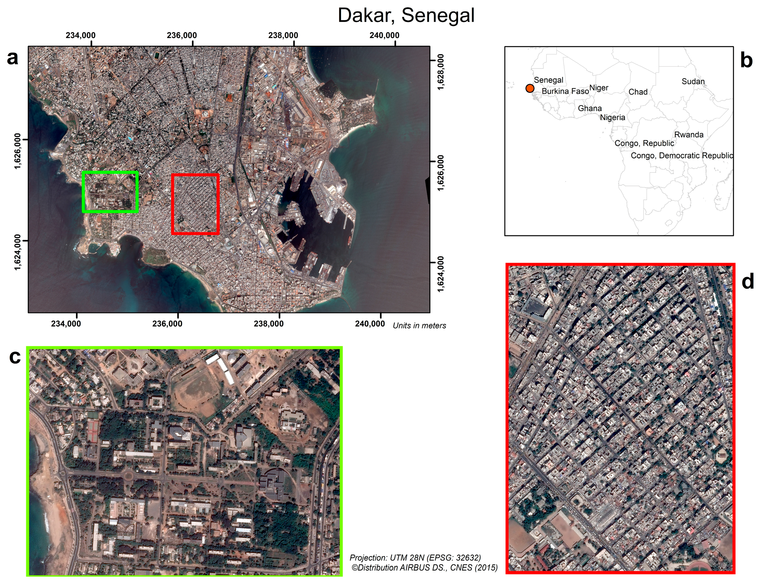
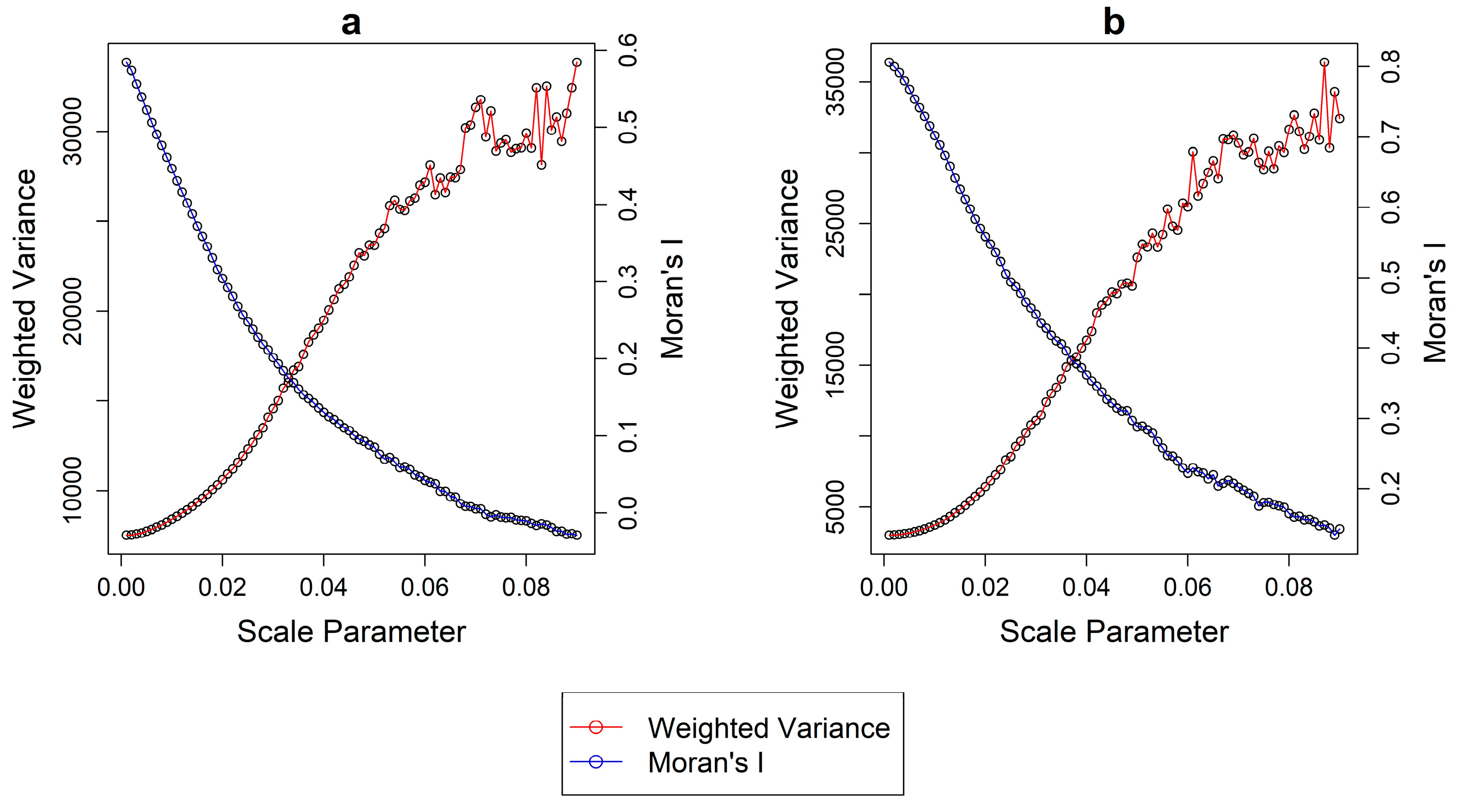
For the traditional implementation of normalization [20] this is not a problem as both WV and MI values are known for each segmentation. To illustrate this, we applied the approach in the two regions of interest (ROI). We computed 90 segmentations with an incrementing scale parameter starting from an extremely fine scale to an extremely coarse one. It should be noted that the scale parameter here is different from the one of eCognition [38]. In the “i.segment” module of GRASS, the decisive merging “threshold” parameter ranges from 0 to 1, with 0 leading to the creation of no segments at all, while 1 represents the merging of all pixels. In the case of the two ROIs in this image, values between 0.001 and 0.09 include all relevant segmentations as suggested by the extreme shift of MI and WV in Figure 2. Finally, a step of 0.001 was used.

Table 1. Absolute maximum and minimum values for the two ROI for the FT method.

Fixed Thresholds	Region 1	Region 2
WVmax	128,314	112,811
WVmin	0	0
MImax	1	1
MImax	−1	−1

shows the absolute values of WV and MI for each case study, respectively. It should be noted that we employed a multiband approach where each of the metrics was computed per single band and then averaged the results [20,34].

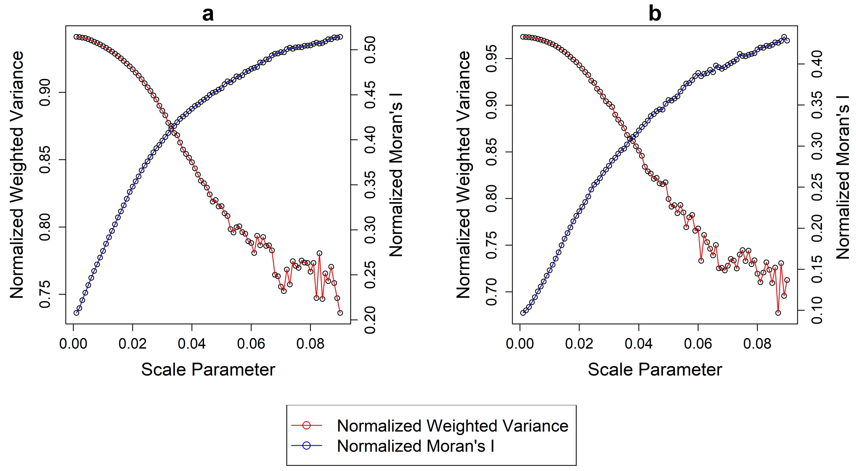
By applying the normalization procedure using these values as the min/max, spurious results were produced. Figure 3 illustrates the Normalized Weighted Variance (WVn) and Normalized Moran’s I (MIn) plotted against each segmentation scale in a similar fashion as before. It is evident that the range of values (i.e., MIn maximum–MIn minimum) of the two metrics is intrinsically different among them and in both regions. The range of WVn for the two regions is 0.20 and 0.29, respectively. On the contrary the same values for MIn are 0.31 and 0.34. In a normalization process, unequal ranges in the values is an indicator of bias towards one or the other metrics. 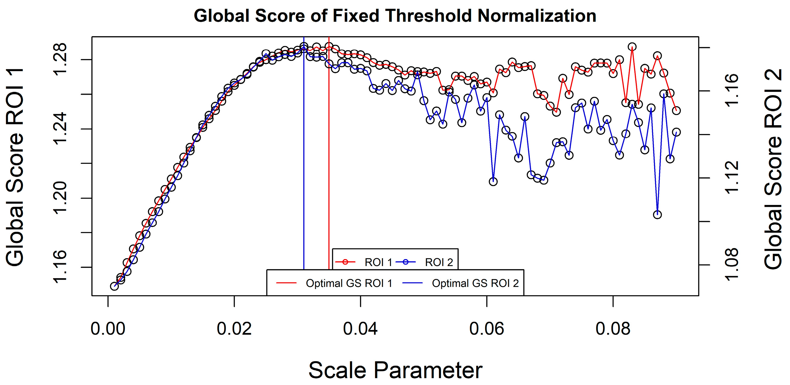This suggests that by using the FT method the GS is biased towards MI (which has a larger range) and as such, segmentations with potentially undersegmented objects might be suggested as optimal. The optimal GS values for ROI 1 was found with a scale parameter of 0.035 while for ROI 2 a scale value of 0.031 was suggested as suitable (Figure 4).

2.3. Selection of Relevant Ranges Based on Local Regression (LOESS) Trend Analysis

Given the methodological concerns that come with the approach described above, an alternative solution is to focus on selecting relevant ranges for the normalization before computing the GS in an objective and meaningful manner. Our proposed solution revolves around detecting variability shifts in the rate of change of WV and MI values. Erratic behavior in these trends can suggest the maximum limit for a reasonable segmentation range to be considered for normalization. The rate of change of variability and autocorrelation metrics such as WV and MI are useful indicators that can detect changes (e.g., shift to oversegmented scales). Drǎguţ et al. [18] used the rate of change in Local Variance to suggest optimal segmentation parameters with the ESP tool. Instead, we are looking for segmentation ranges to apply the traditional GS USPO procedure. 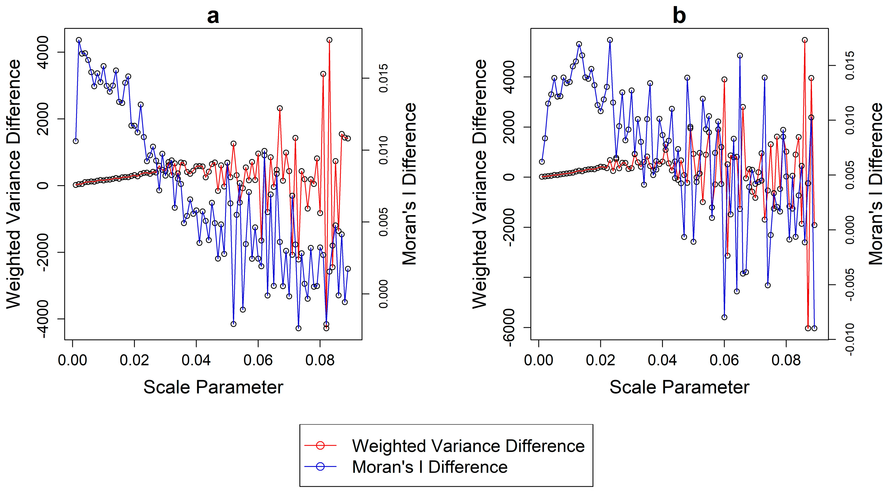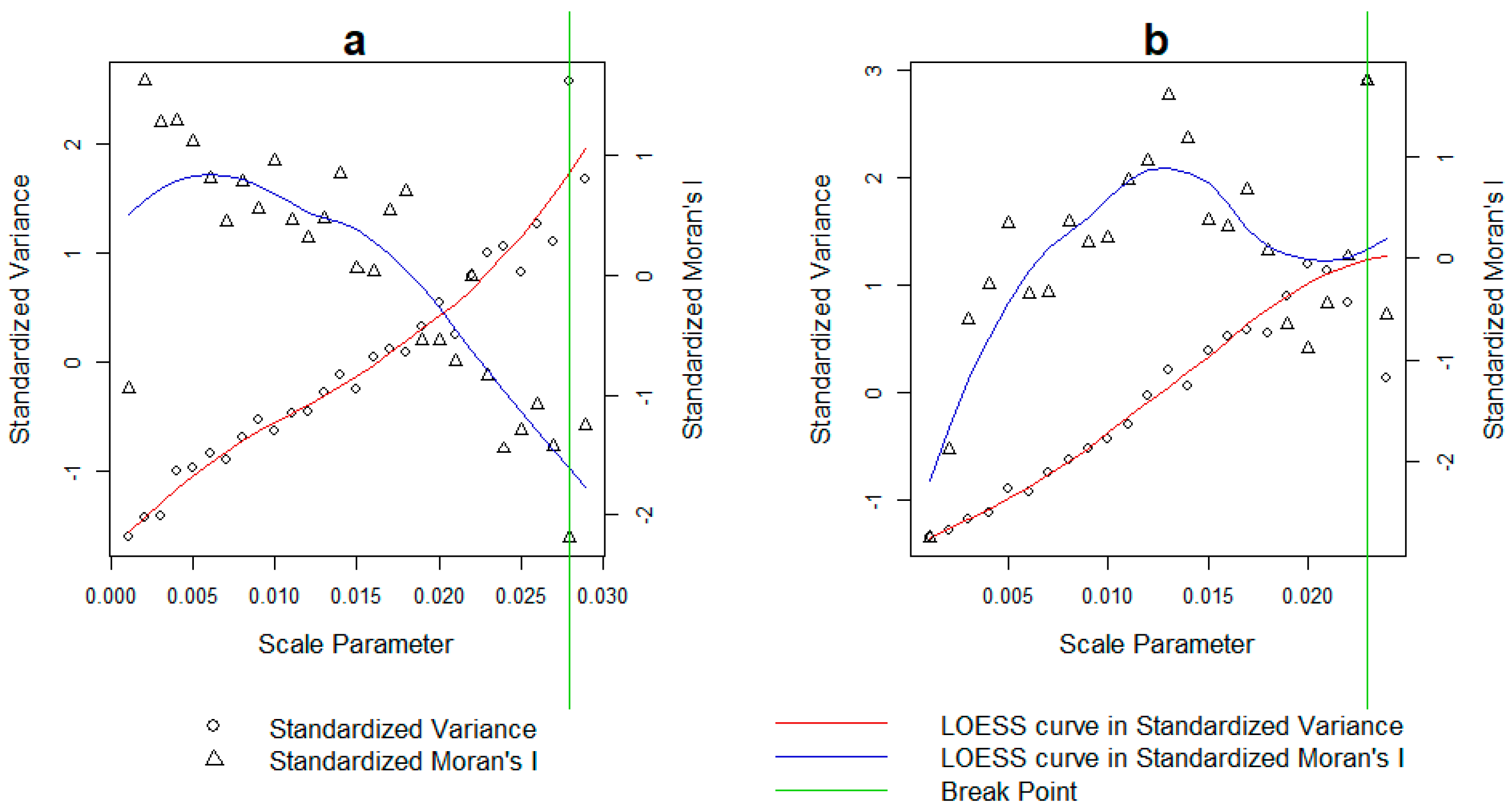Figure 5 shows the difference for each of the two metrics from each segmentation layer and the next and for each ROI, respectively. Notably, erratic behavior and instability is found for both metrics starting at a segmentation scale of 0.020, which becomes apparent visually after a scale value of 0.030 and onwards, in both datasets. Including segmentations beyond this value can add bias to the normalization process as the rates of change for both metrics display an intrinsically unstable behavior. This is due to the large, sudden and irregular changes in the objects size and composition in too heavily undersegmented layers.

Since computing an extremely large amount of segmentations, investigating the trends and visually assessing the point of instability might be a subjective process and time inefficient, we propose an automated solution based on Local Regression (LOESS) curve fitting. LOESS partitions data into subsets and fits a low degree polynomial in each one of them. As a local regression technique, LOESS-based models are suitable methods to detect significant breaks in trends of various data [39]. The salient steps of our solution are described as follows:

• Selection of a segmentation to act as minima (fine scale) and a step value as user-based inputs. A very low scale parameter, which produces very oversegmented results, is appropriate for this task. The results of LOESS are sensitive to the step between each segmentation as the algorithm is more efficient when a lot of data points are given and as such, a very small step parameter is required in order for the trends to manifest. In our case, we used a segmentation produced from a scale parameter of 0.001 as minimum range with the same value as a step. Tests with a step parameter higher than 0.003 failed to provide reasonable results.
• Consider an initial amount of segmentations and compute MI and WV values for each one. For the LOESS curve to produce meaningful results, at least a few segmentations (n~10) should be produced, as it is a local fitting method that operates in subsets of the input data.
• Computing the difference of MI (MI_D) and WV (WV_D) between a segmentation and the next coarser one:

  MI_D = MI_i − MI_i+1

  (5)

  WV_D = WV_i+1 − WV_i

  (6)

  where MI_i is the MI value of the current segmentation and MI_i+1 the value of the next coarser one, and WV_i is the WV value of the current segmentation and WV_i+1 the value of the next coarser one.
• Standardizing the differences of each metric (standard deviation of 1 and mean of 0) as shown in Equation (7):

  $$XDS=(X_D-{\overline{X}}_D)/SD$$

  (7)

  where $X_D$ is the current value for MI_D (or WV_D), ${\overline{X}}_D$ is the mean value of the MI_D (or WV_D) for considered segmentations and SD their standard deviation.
• Fit a LOESS curve to the standardized differences with a second-degree polynomial. The results of the fit are sensitive to the span parameter, which controls the degree of smoothing. The default value (0.75) of the loess package in R statistical software was used.
• Examine the residuals between the LOESS predictions and the raw values. Since the data are standardized, the residuals correspond to standard deviations. Residuals that are sufficiently high for both MI_DS and WV_DS are indicators of a break in the trends. As a rule of thumb, we can assume that a significant shift in the trends manifests when the residuals are higher than 0.4 (larger than 0.4 times a standard deviation) for both MI and WV at the same time while the sum of their absolute residuals is larger than 1. This rule assures both individual and combined evaluation of the trends.
• Selecting the segmentation that satisfies the previous rule as the maximum range. If the criteria are not satisfied, compute an additional coarser segmentation by incrementing the scale parameter, and repeat from step 3.

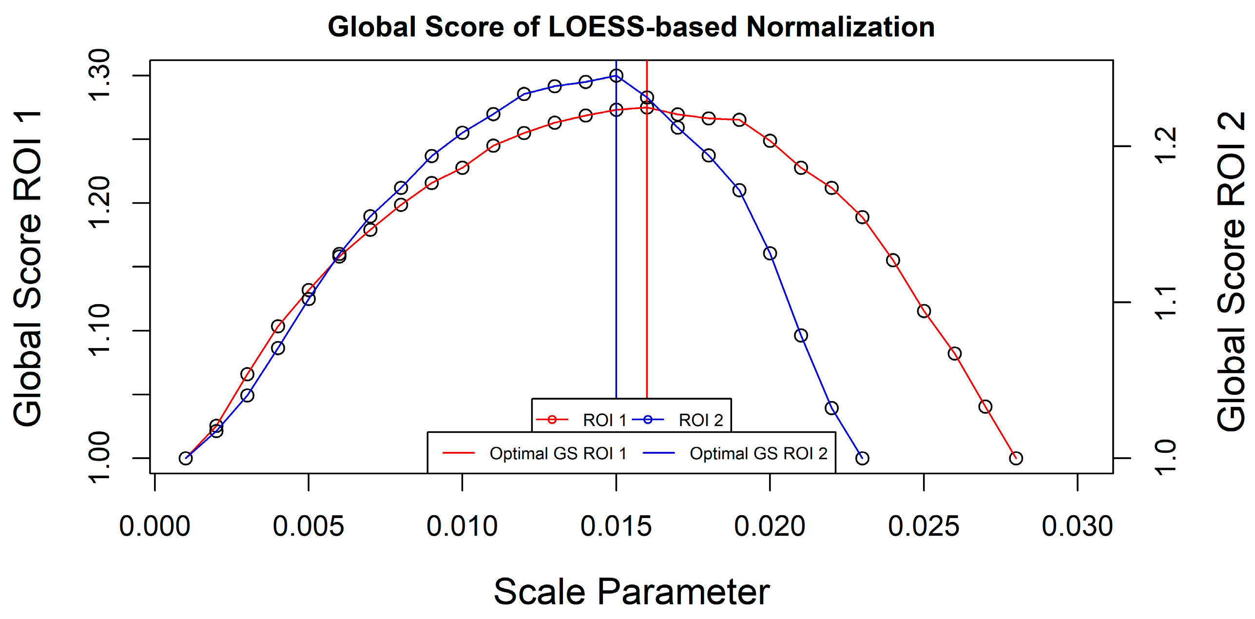
The proposed solution is conservative in nature, as it requires the minimum amount of segmentations to be computed to select an adequate range rather than an arbitrary fixed one. In ROI 1 the criteria were satisfied at a segmentation with a scale parameter of 0.028 (Figure 6). As a reminder, this value represents the maximum value used for the normalization. Applying this value, the optimization of the GS was found at a scale of 0.016 (Figure 7). For the second region, the maximum limit for normalization was 0.023 and the GS was optimized at a segmentation produced with a scale parameter of 0.015.

2.4. Validation Scheme

To investigate the efficiency of the FT approach and the potential improvement of the proposed LOESS technique we employed a two-step validation scheme. First, we computed segmentation goodness metrics (discrepancy measures) to directly measure the quality of each segmentation method. 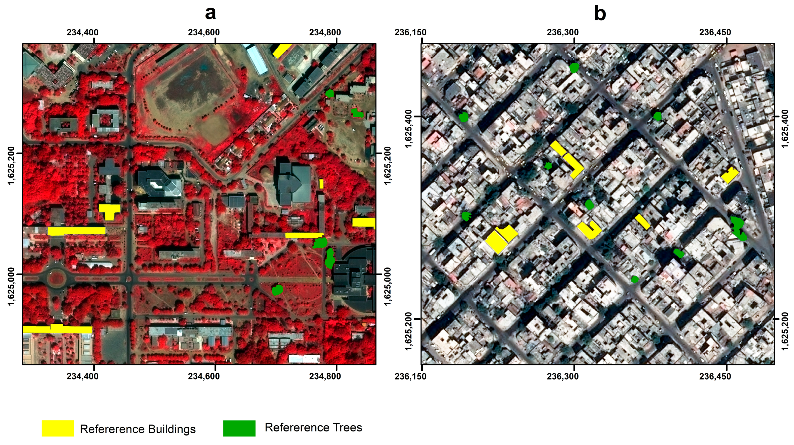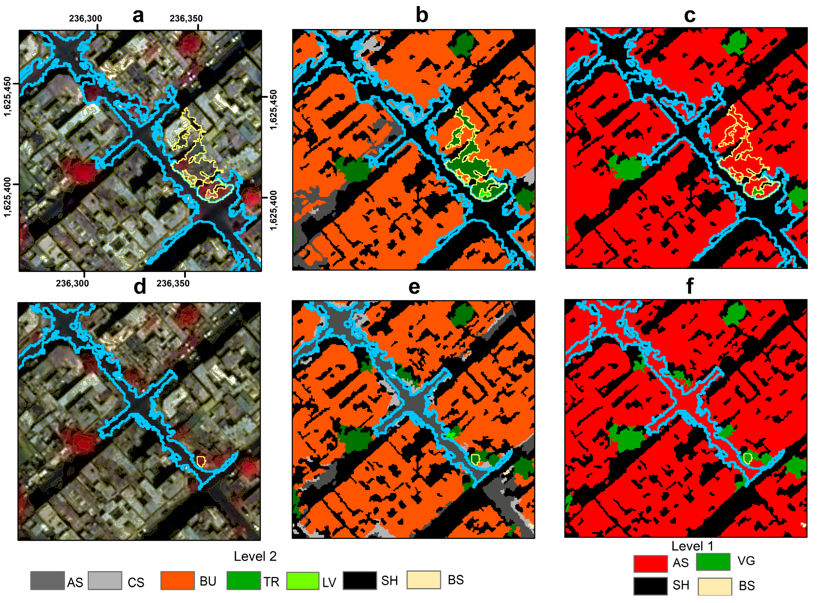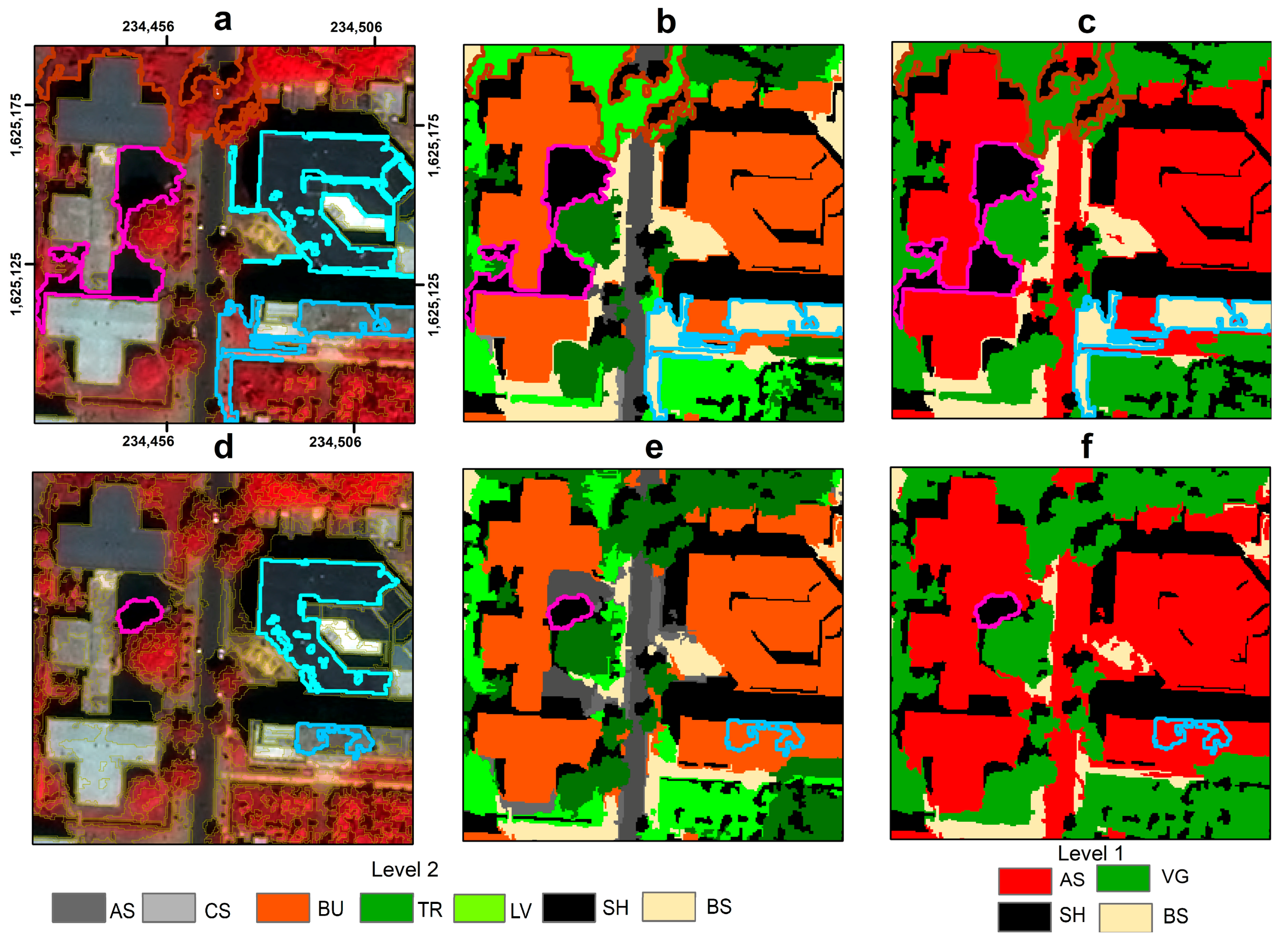These metrics are based on overlaying operations between produced segments and reference objects and are extensively described in several studies [4,16,40,41,42]. We manually digitized 20 objects of interest in each ROI for the buildings and tree categories to serve as reference polygons. The objects were derived from the pool of training data used for LULC classification (Figure 8,

Table 2. Classification scheme and training data for each class.

Level 1	Level 2	Training Samples
Artificial Surface (AS)	Buildings (BU)	91
	Light concrete (CS)	42
	Asphalt (AS)	57
Bare Soil (BS)	Bare Soil (BS)	48
Vegetation (VG)	Trees (TR)	70
	Low Vegetation (LV)	60
Shadow (SH)	Shadow (SH)	71

). Afterwards, we computed the Area Fit Index (AFI) [43], which is an area-based metric and the MergeSum (MS) [16], which is a combined measure that jointly evaluates over/under segmentation. For AFI, values > 0 indicate oversegmentation, values < 0 indicate undersegmentation with the ideal value (perfect fit) being 0. For MS, values closer to 0 indicate a better segmentation performance.

The second measure we used to evaluate the two methods is through the results of a LULC classification of the two ROIs. To do so, we collected 440 points across both ROIs through random sampling and we labeled them according to the specifications of the two-level classification scheme described in Table 2. The objects underlaying the training points received the corresponding class value. Undersegmented objects were discarded, so the training sample size for each method was not exactly the same, as it would depend on the degree of undersegmentation of the image. A Random Forest (RF) classifier was used to perform the classification. Regarding the parameters of the RF models, 500 trees were selected, while the number of features to be examined at each tree node was determined from cross-validation to be 5. We used the complement of the out of the bag error (OOB; ~30% hold out training sample for each tree) as a proxy for the overall accuracy (OA; i.e., OA = 1 − OOB). The OOB has been suggested as a robust metric that can be utilized as an alternative of using an independent test set [44]. For the scope of the study, which is comparative and not aimed on maximizing performance, the OOB was found appropriate as it has been used successfully in recent research [45]. We considered 60 features as input to the classifier and namely descriptive statistics (min, max, median, mean, standard deviation, range, sum, 90th percent, first and third quartiles) for each spectral band, the nDSM and the NDVI, as well as geometrical covariates such as compactness, perimeter and area.

The analysis was performed with an Intel^® Xeon^® CPU E5-2690 (2.90 GHz, 2 processors, 16 cores, 32 processing threads) and 96 GB of RAM. The average time for the “i.segment” module of GRASS to produce a segmentation for a single scale parameter is 34 and 28 s for each ROI, respectively. For performing the USPO procedure as proposed by the authors, roughly 15 (ROI 1) and 11 (ROI 2) minutes are required. This includes the computation of the actual segmentation layer proposed by the USPO as well as descriptive files regarding the MI, WV and GS values for each considered scale parameter. The processing time requirements reported above refer to non-parallelized, single thread versions. If parallelized using the specifications of our hardware, the whole process for both ROIs at the same time would require approximately 4 min.

3. Results

3.1. Segmentation Goodness Metrics

The results of the computed metrics for buildings are depicted in

Table 3. Descriptive statistics for the Area Fit Index (AFI) and MergeSum (MS) metrics for the buildings category based on 20 reference objects.

Descriptive Statistics			Built-Up
	Area Fit Index (AFI)		MergeSum (MS)
	FT	LOESS	FT	LOESS
Mean	−1.64	0.59	1.14	0.96
SD	3.60	0.20	1.24	0.09
1st Quartile	−2.73	0.48	1.24	0.97
3rd Quartile	0.54	0.72	1.00	0.99

. To investigate the distribution of the results in depth, several descriptive statistics are provided. The AFI for the FT approach was mostly negative, indicating that undersegmentation was prevalent, while the large value of the standard deviation (SD) demonstrates the instability in the size of the segments relative to the size of the objects of interest. On the contrary, the LOESS-based technique was consistently positive and with values closer to 0. In a similar fashion, the MS metric values were lower for the proposed method with a smaller SD.

Similar results for the trees as objects of interest are shown in

Table 4. Descriptive statistics for the Area Fit Index (AFI) and MergeSum (MS) metrics for the trees category based on 20 reference objects.

Descriptive Statistics			Trees
	Area Fit Index (AFI)		MergeSum (MS)
	FT	LOESS	FT	LOESS
Mean	−50.81	0.53	24.69	0.91
SD	113.74	0.23	79.97	0.14
1st Quartile	−26.42	0.37	0.82	0.89
3rd Quartile	0.19	0.69	2.05	0.99

. The reason for the extreme negative values of the AFI and MS for the FT approach is the frequent merging of tree objects with very large segments that represent asphalted streets or bare soil in both ROI.

Examples of the two segmentation methods are demonstrated in Figure 9 where scenes of different built-up densities and size are visualized. Figure 9a,b represents a built-up area of medium size, high density belonging to the first ROI. It is evident that the FT normalization produced extremely undersegmented objects, mixing multiple LULC classes such as vegetation with artificial surfaces. To ease interpretability, for FT, we highlight particularly large objects, which combine different types of vegetation, bare soil, built-up areas, shadows and asphalt. On the contrary, the segmentation derived from LOESS did not appear undersegmented, and clear separation between different LULC categories was observed (highlighted objects). In a similar fashion, in the examples from the second ROI (Figure 9c,d), segmentations coming from the fixed approach were severely undersegmented while the proposed solution produced distinct objects with a particular benefit for buildings, as they were not combined with ground level concrete surfaces. In general, it can be pointed out that due to the very large scale parameter that FT identified as optimum, unless there was a clear spectral separation between neighboring objects, segments consisting of several LULC classes were created.

3.2. Classification Results

As an indirect evaluation of the two methods, the OA calculations for the two-level LULC classifications produced using each method are presented in

Table 5. Overall accuracies (OA) for two levels using different segmentations as input.

Classification Scheme	Level 1		Level 2
Optimization Method	FT	LOESS	FT	LOESS
Overall Accuracy (%)	88.08	94.34	77.24	88.68
Kappa Index	0.83	0.92	0.72	0.87

. In line with the previous results (Section 3.1), the LOESS technique produced significantly higher OAs for both classification levels. At Level 1 LOESS exhibited roughly a 6% increase in OA in comparison to the FT method. Notably, at Level 2 the improvement was even higher (~10%), probably because accurate context information (e.g., segment area and shape) was particularly important for distinguishing buildings and trees. Finally, the F-score as a measure of per class accuracy is presented for each segmentation method and classification level (

Table 6. F-score for each class for each classification level and segmentation method.

Class	Level 1		Class	Level 2
	FT	LOESS		FT	LOESS
Artificial Surface	0.91	0.95	Asphalt	0.69	0.84
Vegetation	0.92	0.97	Buildings	0.85	0.90
Bare Soil	0.71	0.86	Light concrete	0.43	0.70
Shadow	0.90	0.96	Bare Soil	0.75	0.82
			Trees	0.83	0.90
			Low Vegetation	0.75	0.88
			Shadow	0.91	0.96

). The degree of improvement of the LOESS method degree varied as a function of class and classification scheme but in all cases, there were large and significant improvements.

Examples of the LULC classification produced from each method are shown in Figure 10 and Figure 11. It is evident that the extreme undersegmentation of the FT method has a strong negative effect in the classification. Figure 10 highlights misclassifications of unclassified land due to shadows with asphalted surfaces and vegetation with built-up areas. LOESS mitigates these problems as the LULC maps are more accurate regardless of the classification scheme used. Regardless of the classification scheme employed, the classifications are evidently better and more consistent. On the contrary, the instability of the FT approach can be seen as objects were classified differently according to each level (e.g., highlighted segments in bright yellow in Figure 10b,c. The results were similar in ROI 2 (Figure 11). The highlighted objects with FT emphasize situations of asphalt/shadows confusion, bare soil/built-up as well as confusion between different types of vegetation.

4. Discussion

As this experiment of the study demonstrated, there are important limitations arising using fixed threshold values for the normalization process in VHR urban scenes. The most important disadvantage is that by doing so, both metrics are unequally weighted, with MI typically having greater weighting, due to the fact that the absolute value ranges of each metric are quite different as MI has a smaller range of possible values than WV. This has explicit effects on the normalization procedure, especially when unrealistic ranges are imposed. Indeed, the results on an empirical application were quite clear—segmentations identified as “optimal” from this procedure were actually highly undersegmented. Moreover, this also renders the implementation of other intrasegment/intersegment heterogeneity combination approaches, e.g., those based on the F-measure [20], inapplicable, as the already unequal normalized metric values would be inflated further. The results could arguably be improved if better fixed values were selected, rather than simply selecting the extreme values for each metric. Nonetheless, this would make the problem sensitive to the search range, the same issue it is supposed to solve.

Previous studies showed that results from subjectively selecting ranges were adequate [29,34,46]. Indeed, selecting ranges based on user experience, together with a clear aim linked to the purpose of the expected outcome of the analysis (e.g., minimum mapping units, classification scheme), can lead to high quality of the results. Nonetheless, this process is still subjective and requires sufficient experimentation to define the appropriate ranges, something that goes against the rationale of using USPO methods in the first place, especially with the aim of automation in mind. Moreover, it can be time inefficient, particularly for large datasets. Therefore, we propose a solution that focuses on selecting a relevant range of values for normalizations by detecting trend instability in the rates of change of MI and WV. The proposed solution through LOESS curve fitting appears to provide adequate results for VHR data of different types of urban LULC.

In order for the proposed method to identify optimal segmentations at different scales several options could be investigated. A multiscale analysis by adjusting the weight parameter of the F-measure formula can be undertaken in a similar fashion as demonstrated by Johnson et al. [20]. An alternative way would be to run the LOESS with the proposed specifications, detect the scale parameter of the break point and re-run the procedure using it as the starting segmentation scale until it identifies a second breakpoint. Finally, adjusting the minimum size of the produced segments by the region-growing algorithm of the “i.segment” tool of GRASS according to the minimum mapping units of different LULC classification schemes could potentially address the issue of detecting image units at different semantic levels.

An important advantage of the proposed method is its potential for automation with particular merit for large, heterogeneous areas. As Grippa et al. [47] and Georganos et al. [48] pointed out, in heterogeneous urban scenes a single set of segmentation parameters is inadequate and less efficient than spatially partitioning the study area into several subsets and optimizing each separately. Similar studies for semi-rural and agricultural environments have demonstrated the efficacy of local optimization through the use of F-measure and ESP methods [25,27]. In these cases, undertaking supervised methods would be largely untenable and inefficient while traditional USPO methods would rely on setting defined segmentation ranges a priory. On the other hand, the proposed method can provide a fully automated procedure for selecting relevant ranges for each subset (providing parameters such as the starting segmentation scale have been defined according to the application specifications). This works in a synergistic fashion with GRASS GIS, which is suited for large-scale computing, is highly automated and parallelized in most of its functions and more importantly, performs all the segmentation operations in a raster format without involving vector data unless requested, which dramatically boosts its computational efficiency. Nonetheless, further research is needed with different types of algorithm parametrization, imagery, classification schemes and objectives to validate the efficacy of LOESS as an adequate method for addressing normalization issues in the computation of the GS and similar measures. Finally, comparisons with other highly automated USPO methods such as the ESP tool of eCognition [18] should be investigated.

5. Conclusions

Unsupervised segmentation parameter optimization (USPO) is typically done by identifying the segmentation (out of a set of candidate segmentations) with the highest combined intersegment heterogeneity and intrasegment homogeneity (i.e., the “optimal” segmentation). Global Moran’s I (MI) (an intersegment heterogeneity metric) and area-weighted variance (WV) (an intrasegment heterogeneity measure) values are often combined for this purpose, and an “optimal” segmentation is identified based on the combined result; i.e., the “Global Score” (GS) values of the candidate segmentations. Recent research demonstrated in detail that the values of GS are dependent on the range of candidate segmentations because the MI and WV values are normalized prior to being combined. As a remedy a normalization of the MI and WV values based on fixed minimum/maximum values was proposed (FT).

In this study, we investigated the efficiency of the (FT) both theoretically and empirically and alternatively proposed performing the normalization through Local Regression Trend Analysis (LOESS) methods. From our analysis, it was demonstrated that the FT is susceptible to unequal weighting of the metrics that are used for normalization (i.e., Moran’s I and Weighted Variance). We empirically validated the results through segmentation goodness metrics such as the Area Fit Index (AFI) and MergeSum, which indicated heavy undersegmentation while LOESS showed no such signs. We additionally demonstrated these issues in a two-level Land-Use/Land-Cover classification scheme where GS optimized through LOESS largely overperformed in terms of Overall Accuracy (~6% for level 1 and ~10% at level 2). Finally, we emphasize the objectivity and benefits of semi- or fully automated USPO methods that do not rely heavily on user interference to define the segmentation ranges, further supporting the rationale of using USPO methods, especially for large heterogeneous areas.

References

1. Walter, V. Object-based classification of remote sensing data for change detection. ISPRS J. Photogramm. Remote Sens. 2004, 58, 225–238. [Google Scholar] [CrossRef]
2. Blaschke, T.; Hay, G.J.; Kelly, M.; Lang, S.; Hofmann, P.; Addink, E.; Queiroz Feitosa, R.; van der Meer, F.; van der Werff, H.; van Coillie, F.; et al. Geographic Object-Based Image Analysis-Towards a new paradigm. ISPRS J. Photogramm. Remote Sens. 2014, 87, 180–191. [Google Scholar] [CrossRef] [PubMed]
3. Carleer, A.P.; Wolff, E. Urban land cover multi-level region-based classification of VHR data by selecting relevant features. Int. J. Remote Sens. 2006, 27, 1035–1051. [Google Scholar] [CrossRef]
4. Whiteside, T.G.; Boggs, G.S.; Maier, S.W. Comparing object-based and pixel-based classifications for mapping savannas. Int. J. Appl. Earth Obs. Geoinf. 2011, 13, 884–893. [Google Scholar] [CrossRef]
5. Meneguzzo, D.M.; Liknes, G.C.; Nelson, M.D. Mapping trees outside forests using high-resolution aerial imagery: A comparison of pixel- and object-based classification approaches. Environ. Monit. Assess. 2013, 185, 6261–6275. [Google Scholar] [CrossRef] [PubMed]
6. Blaschke, T. Object based image analysis for remote sensing. ISPRS J. Photogramm. Remote Sens. 2010, 65, 2–16. [Google Scholar] [CrossRef]
7. Gao, Y.A.N.; Mas, J.F.; Kerle, N.; Navarrete Pacheco, J.A. Optimal region growing segmentation and its effect on classification accuracy. Int. J. Remote Sens. 2011, 32, 3747–3763. [Google Scholar] [CrossRef]
8. Baumgartner, J.; Gimenez, J.; Scavuzzo, M.; Pucheta, J. A New Approach to Segmentation of Multispectral Remote Sensing Images Based on MRF. IEEE Geosci. Remote Sens. Lett. 2015, 12, 1720–1724. [Google Scholar] [CrossRef]
9. Belgiu, M.; Drǎguţ, L. Comparing supervised and unsupervised multiresolution segmentation approaches for extracting buildings from very high resolution imagery. ISPRS J. Photogramm. Remote Sens. 2014, 96, 67–75. [Google Scholar] [CrossRef] [PubMed]
10. Kohli, D.; Crommelinck, S.; Bennett, R.; Koeva, M.; Lemmen, C. Object-based image analysis for cadastral mapping using satellite images. In Proceedings of the International Society for Optics and Photonics, Image Signal Processing Remote Sensing XXIII, Warsaw, Poland, 4 October 2017; Volume 10427, p. 104270V. [Google Scholar]
11. Li, F.; Wong, A.; Clausi, D.A. Comparison of unsupervised segmentation methods for surficial materials mapping in Nunavut, Canada using RADARSAT-2 polarimetric, Landsat-7, and DEM data. In Proceedings of the 2014 IEEE International Geoscience and Remote Sensing Symposium (IGARSS), Quebec City, QC, Canada, 13–18 July 2014; pp. 2727–2730. [Google Scholar]
12. Troya-Galvis, A.; Gancarski, P.; Passat, N.; Berti-Équille, L. Unsupervised quantification of under-and over-segmentation for object-based remote sensing image analysis. IEEE J. Sel. Top. Appl. Earth Obs. Remote Sens. 2015, 8, 1936–1945. [Google Scholar] [CrossRef]
13. Wang, M.; Dong, Z.; Cheng, Y.; Li, D. Optimal Segmentation of High-Resolution Remote Sensing Image by Combining Superpixels With the Minimum Spanning Tree. IEEE Trans. Geosci. Remote Sens. 2017, 56, 228–238. [Google Scholar] [CrossRef]
14. Jozdani, S.E.; Momeni, M.; Johnson, B.A.; Sattari, M. A regression modelling approach for optimizing segmentation scale parameters to extract buildings of different sizes. Int. J. Remote Sens. 2018, 39, 684–703. [Google Scholar] [CrossRef]
15. Aguilar, M.A.; Novelli, A.; Nemamoui, A.; Aguilar, F.J.; Lorca, A.G.; González-Yebra, Ó. Optimizing Multiresolution Segmentation for Extracting Plastic Greenhouses from WorldView-3 Imagery. In Proceedings of the International Conference on Intelligent Interactive Multimedia Systems and Services, Vilamoura, Portugal, 21–23 June 2017; pp. 31–40. [Google Scholar]
16. Clinton, N.; Holt, A.; Scarborough, J.; Yan, L.; Gong, P. Accuracy assessment measures for object-based image segmentation goodness. Photogramm. Eng. Remote Sens. 2010, 76, 289–299. [Google Scholar] [CrossRef]
17. Rasanen, A.; Rusanen, A.; Kuitunen, M.; Lensu, A. What makes segmentation good? A case study in boreal forest habitat mapping. Int. J. Remote Sens. 2013, 34, 8603–8627. [Google Scholar] [CrossRef]
18. Drǎguţ, L.; Tiede, D.; Levick, S.R. ESP: A tool to estimate scale parameter for multiresolution image segmentation of remotely sensed data. Int. J. Geogr. Inf. Sci. 2010, 24, 859–871. [Google Scholar] [CrossRef]
19. Espindola, G.M.; Camara, G.; Reis, I.A.; Bins, L.S.; Monteiro, A.M. Parameter selection for region-growing image segmentation algorithms using spatial autocorrelation. Int. J. Remote Sens. 2006, 27, 3035–3040. [Google Scholar] [CrossRef]
20. Johnson, B.; Bragais, M.; Endo, I.; Magcale-Macandog, D.; Macandog, P. Image Segmentation Parameter Optimization Considering Within- and Between-Segment Heterogeneity at Multiple Scale Levels: Test Case for Mapping Residential Areas Using Landsat Imagery. ISPRS Int. J. Geo-Inf. 2015, 4, 2292–2305. [Google Scholar] [CrossRef]
21. Chabrier, S.; Emile, B.; Rosenberger, C.; Laurent, H. Unsupervised performance evaluation of image segmentation. EURASIP J. Appl. Signal Process. 2006, 2006, 217. [Google Scholar] [CrossRef]
22. Sublime, J.; Troya-Galvis, A.; Puissant, A. Multi-scale analysis of very high resolution satellite images using unsupervised techniques. Remote Sens. 2017, 9, 495. [Google Scholar] [CrossRef]
23. Gao, H.; Tang, Y.; Jing, L.; Li, H.; Ding, H. A Novel Unsupervised Segmentation Quality Evaluation Method for Remote Sensing Images. Sensors 2017, 17, 2427. [Google Scholar] [CrossRef] [PubMed]
24. Georganos, S.; Grippa, T.; Vanhuysse, S.; Lennert, M.; Shimoni, M.; Kalogirou, S.; Wolff, E. Less is more: optimizing classification performance through feature selection in a very-high-resolution remote sensing object-based urban application. GISci. Remote Sens. 2017. [Google Scholar] [CrossRef]
25. Kavzoglu, T.; Erdemir, M.Y.; Tonbul, H. Classification of semiurban landscapes from very high-resolution satellite images using a regionalized multiscale segmentation approach. J. Appl. Remote Sens. 2017, 11, 35016. [Google Scholar] [CrossRef]
26. Grippa, T.; Lennert, M.; Beaumont, B.; Vanhuysse, S.; Stephenne, N.; Wolff, E. An open-source semi-automated processing chain for uban OBIA classification. In Proceedings of the GEOBIA 2016 Conference Mach-2 Machine Learning & Automation II, Enschede, The Netherlands, 14–16 September 2016; pp. 1–6. [Google Scholar]
27. Cánovas-García, F.; Alonso-Sarría, F. A local approach to optimize the scale parameter in multiresolution segmentation for multispectral imagery. Geocarto Int. 2015, 30, 937–961. [Google Scholar] [CrossRef]
28. Vamsee, A.M.; Kamala, P.; Martha, T.R.; Kumar, K.V.; Amminedu, E. A Tool Assessing Optimal Multi-Scale Image Segmentation. J. Indian Soc. Remote Sens. 2017, 46, 31–41. [Google Scholar] [CrossRef]
29. Johnson, B.; Xie, Z. Unsupervised image segmentation evaluation and refinement using a multi-scale approach. ISPRS J. Photogramm. Remote Sens. 2011, 66, 473–483. [Google Scholar] [CrossRef]
30. Wang, C.; Xu, W.; Pei, X.; Zhou, X. An unsupervised multi-scale segmentation method based on automated parameterization. Arab. J. Geosci. 2016, 9, 651. [Google Scholar] [CrossRef]
31. Böck, S.; Immitzer, M.; Atzberger, C. On the Objectivity of the Objective Function—Problems with Unsupervised Segmentation Evaluation Based on Global Score and a Possible Remedy. Remote Sens. 2017, 9, 769. [Google Scholar] [CrossRef]
32. Neteler, M.; Bowman, M.H.; Landa, M.; Metz, M. GRASS GIS: A multi-purpose open source GIS. Environ. Model. Softw. 2012, 31, 124–130. [Google Scholar] [CrossRef]
33. Momsen, E.; Metz, M.; GRASS Development TEAM. Module i.segment 2015. Available online: https://grass.osgeo.org/grass75/manuals/i.segment.html (accessed on 16 August 2017).
34. Grippa, T.; Lennert, M.; Beaumont, B.; Vanhuysse, S.; Stephenne, N.; Wolff, E. An Open-Source Semi-Automated Processing Chain for Urban Object-Based Classification. Remote Sens. 2017, 9, 358. [Google Scholar] [CrossRef]
35. Cliff, A.; Ord, K. Testing for spatial autocorrelation among regression residuals. Geogr. Anal. 1972, 4, 267–284. [Google Scholar] [CrossRef]
36. Kalogirou, S.; Hatzichristos, T. A spatial modelling framework for income estimation. Spat. Econ. Anal. 2007, 2, 297–316. [Google Scholar] [CrossRef]
37. Anselin, L. GeoDaTM 0.9 user’s guide. Urbana 2003, 51, 61801. [Google Scholar]
38. Baatz, M.; Schape, A. Multiresolution Segmentation: An Optimization Approach for High Quality Multi-Scale Image Segmentation. 2000. Available online: https://www.semanticscholar.org/paper/Multiresolution-Segmentation-an-optimization-appro-Baatz-Sch%C3%A4pe/364cc1ff514a2e11d21a101dc072575e5487d17e (accessed on 20 December 2017).
39. Verbesselt, J.; Hyndman, R.; Newnham, G.; Culvenor, D. Detecting trend and seasonal changes in satellite image time series. Remote Sens. Environ. 2010, 114, 106–115. [Google Scholar] [CrossRef]
40. Persello, C.; Bruzzone, L. A novel protocol for accuracy assessment in classification of very high resolution images. IEEE Trans. Geosci. Remote Sens. 2010, 48, 1232–1244. [Google Scholar] [CrossRef]
41. Möller, M.; Birger, J.; Gidudu, A.; Gläßer, C. A framework for the geometric accuracy assessment of classified objects. Int. J. Remote Sens. 2013, 34, 8685–8698. [Google Scholar] [CrossRef]
42. Costa, H.; Foody, G.M.; Boyd, D.S. Remote Sensing of Environment Supervised methods of image segmentation accuracy assessment in land cover mapping. Remote Sens. Environ. 2018, 205, 338–351. [Google Scholar] [CrossRef]
43. Lucieer, A.; Stein, A. Existential uncertainty of spatial objects segmented from satellite sensor imagery. IEEE Trans. Geosci. Remote Sens. 2002, 40, 2518–2521. [Google Scholar] [CrossRef]
44. Breiman, L. Random forests. Mach. Learn. 2001, 45, 5–32. [Google Scholar] [CrossRef]
45. Schultz, B.; Immitzer, M.; Formaggio, A.R.; Sanches, I.D.A.; Luiz, A.J.B.; Atzberger, C. Self-guided segmentation and classification of multi-temporal Landsat 8 images for crop type mapping in Southeastern Brazil. Remote Sens. 2015, 7, 14482–14508. [Google Scholar] [CrossRef]
46. Grybas, H.; Melendy, L.; Congalton, R.G. A comparison of unsupervised segmentation parameter optimization approaches using moderate- and high-resolution imagery. GISci. Remote Sens. 2017, 54. [Google Scholar] [CrossRef]
47. Grippa, T.; Georganos, S.; Lennert, M.; Vanhuysse, S.; Wolff, E. A local segmentation parameter optimization approach for mapping heterogeneous urban environments using VHR imagery. In Proceedings of the SPIE Remote Sensing Technologies and Applications in Urban Environments II, Warsaw, Poland, 4 October 2017. [Google Scholar] [CrossRef]
48. Georganos, S.; Grippa, T.; Lennert, M.; Vanhuysse, S.G.; Wolff, E. SPUSPO: Spatially Partitioned Unsupervised Segmentation Parameter Optimization for Efficiently Segmenting Large Heteregeneous Areas. In Proceedings of the 2017 Conference on Big Data from Space (BiDS’17), Toulouse, France, 28–30 November 2017; p. 4. [Google Scholar]
Figure 1. (a) Pleiades image of Dakar (RGB composite), (b) location map of Dakar within the African continent, (c) ROI 1 (1.05 km2), representing a low-density large size built-up zone and (d) ROI 2 (0.82 km2), representing a high-density medium sized built-up zone.
Remotesensing 10 00222 g001
Figure 2. MI and WV values for each computed segmentation for (a) ROI 1 and (b) ROI 2.
Remotesensing 10 00222 g002
Figure 3. Normalized MI and WV values for each computed segmentation for (a) ROI 1 and (b) ROI 2 using the FT approach.
Remotesensing 10 00222 g003
Figure 4. GS for each computed segmentation and ROI using the FT approach.
Remotesensing 10 00222 g004
Figure 5. Differences in MI and WV between each computed segmentation and the next for (a) ROI 1 and (b) ROI 2.
Remotesensing 10 00222 g005
Figure 6. LOESS curve results for the two ROIs. The breakpoint signifies the point where the absolute residuals are larger than 0.4 standard deviations for both Variance and Moran’s I and their sum greater than 1. In ROI 1 (a) the breakpoint was found with a scale parameter of 0.028 while in ROI 2 (b) a parameter of 0.023 was identified as suitable.
Remotesensing 10 00222 g006
Figure 7. GS for each computed segmentation and ROI using the LOESS approach.
Remotesensing 10 00222 g007
Figure 8. Examples of digitized buildings and trees for the computation of segmentation goodness metrics in (a) ROI 1 and (b) ROI 2.
Remotesensing 10 00222 g008
Figure 9. Example of segmentation results for the two ROI. (a,c) FT approach, (b,d) LOESS approach. Highlighted objects in color other than yellow display undersegmented areas where several LULC classes are mixed for the FT approach, while colored objects in the LOESS case showcase some of the clear improvements as the objects now represent discrete LULC classes (e.g., asphalt, vegetation, building).
Remotesensing 10 00222 g009
Figure 10. Classification results for the two approaches at two levels from ROI 1. (a) Segmentation and highlighted objects from the FT method, (b) classification results for Classification Level 2 and (c) Classification Level 1 for FT, (d) Segmentation and highlighted objects from the LOESS method, (e) classification results for Classification Level 2 and (f) Classification level 1 for LOESS.
Remotesensing 10 00222 g010
Figure 11. Classification results for the two approaches at two levels from ROI 1. (a) Segmentation and highlighted objects from the FT method, (b) classification results for Classification Level 2 and (c) Classification Level 1 for FT, (d) Segmentation and highlighted objects from the LOESS method, (e) classification results for Classification Level 2 and (f) Classification level 1 for LOESS.
Remotesensing 10 00222 g011