Validation of Carbon Monoxide Total Column Retrievals from SCIAMACHY Observations with NDACC/TCCON Ground-Based Measurements


Abstract
:
1. Introduction
1.1. The Environmental Satellite (ENVISAT) and Scanning Imaging Absorption Spectrometer for Atmospheric Chartography (SCIAMACHY) Instrument
1.2. Carbon Monoxide (CO) from Channel 8 of SCIAMACHY
1.3. Retrieval Codes
1.4. The Network for the Detection of Atmospheric Composition Change (NDACC) and Total Carbon Column Observing Network (TCCON) Ground Truthing Networks
1.5. Validation
1.5.1. General Aspects
1.5.2. The SCIAMACHY CO Product
1.6. Goals and Structure of this Study
2. Methodology
2.1. Ground-Based Product Definition
2.1.1. NDACC
2.1.2. The TCCON
2.2. The BIRRA
2.2.1. Algorithm
2.2.2. Product Definition
2.3. Weighted Averages
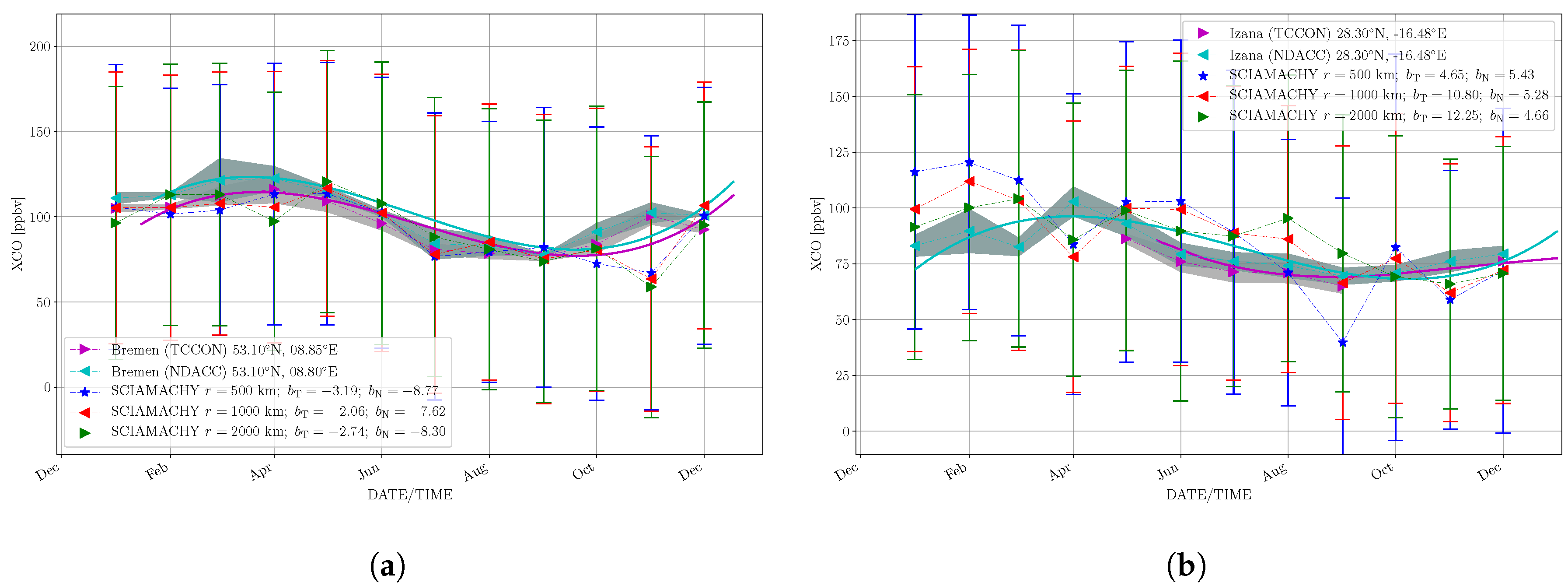
2.3.1. Space
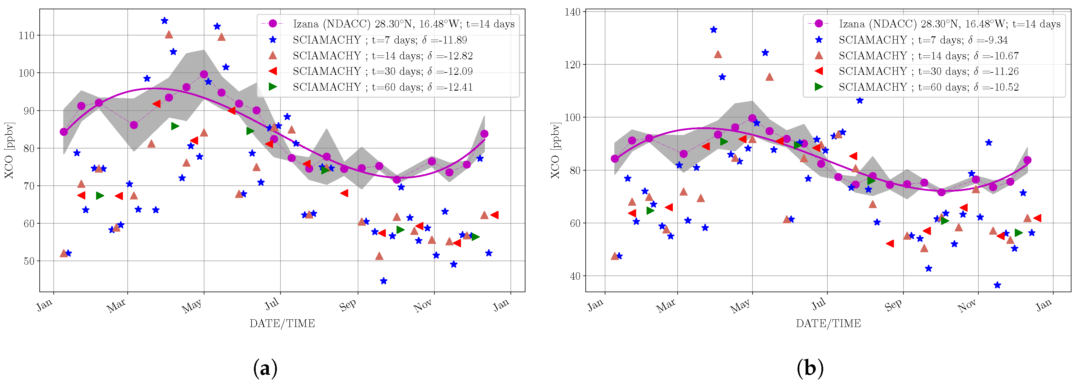
2.3.2. Time
2.4. Bias
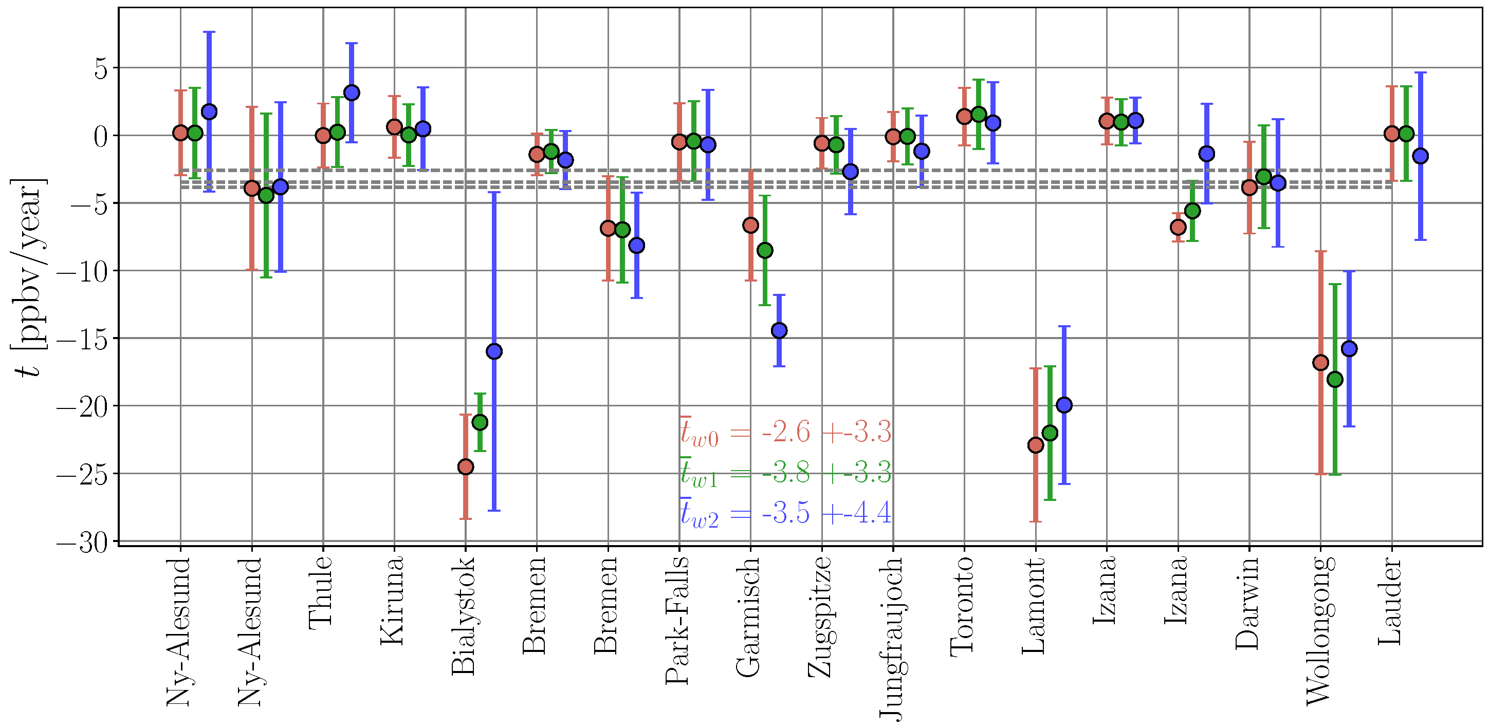
2.5. Averaging Multiple Years of CO
3. Results
3.1. Averaging of Measurements
3.2. Bias and Weighting
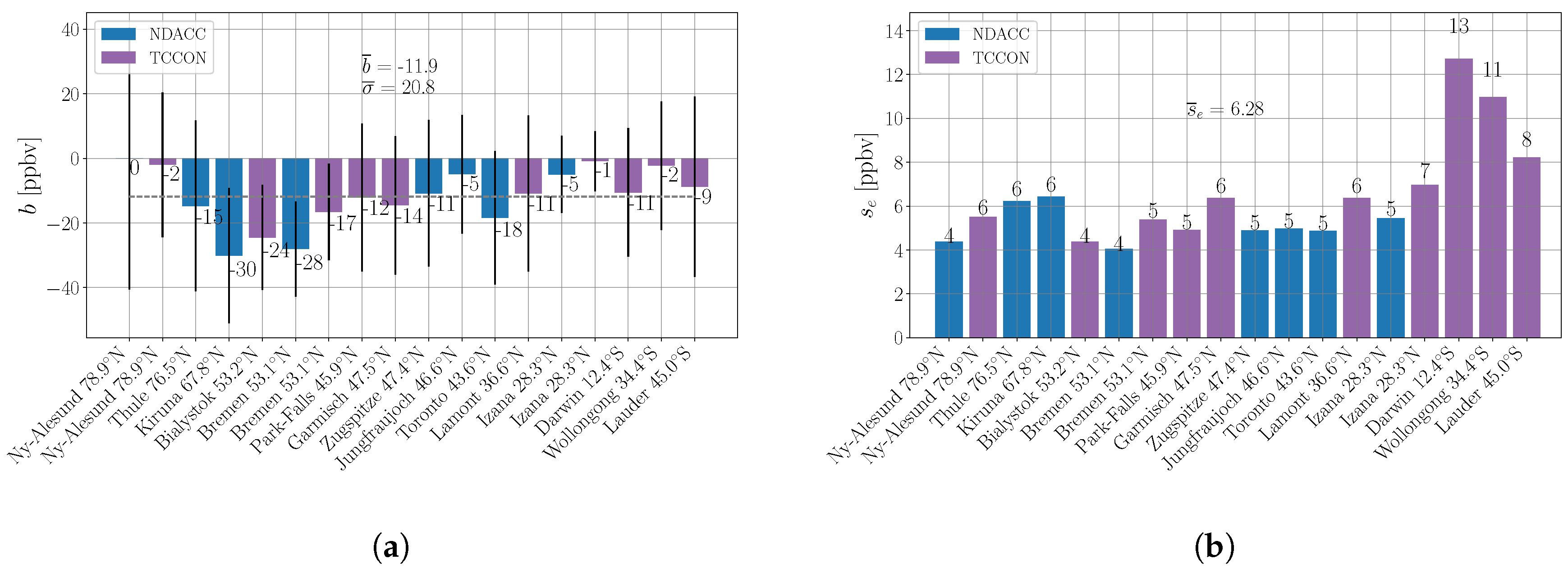
3.2.1. Unweighted Bias
3.2.2. Distance Weighted Bias
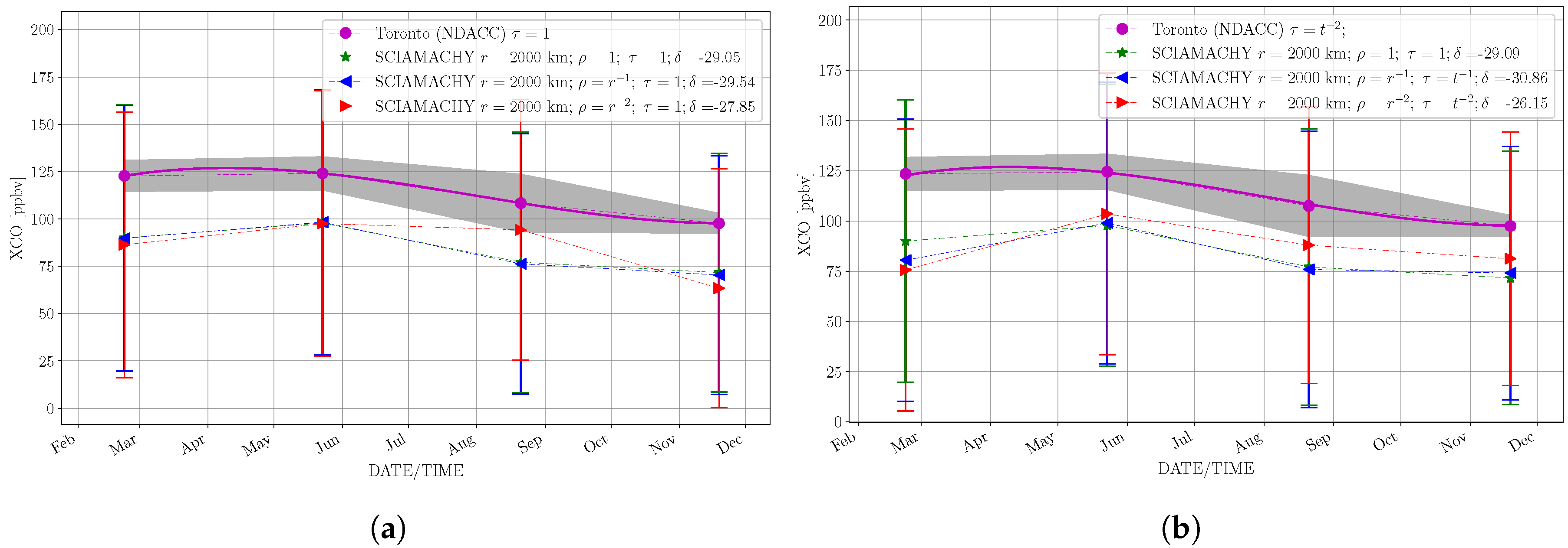
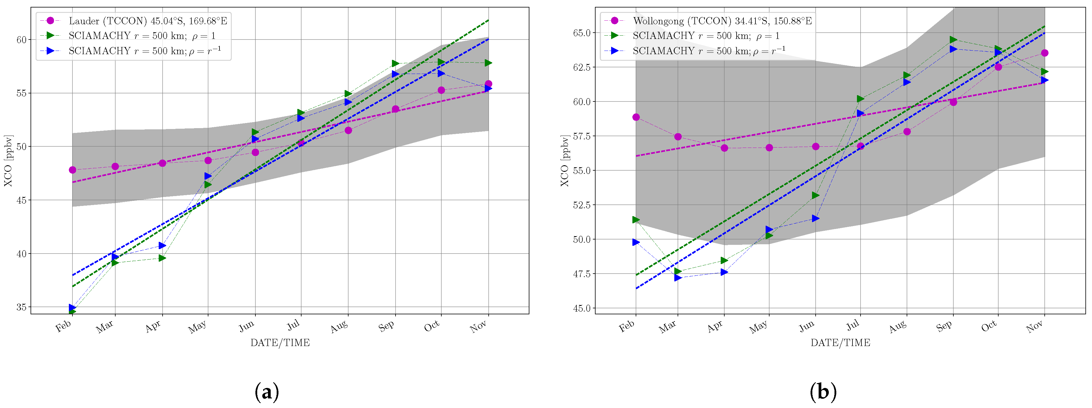
3.2.3. Spatio-Temporal Weighting
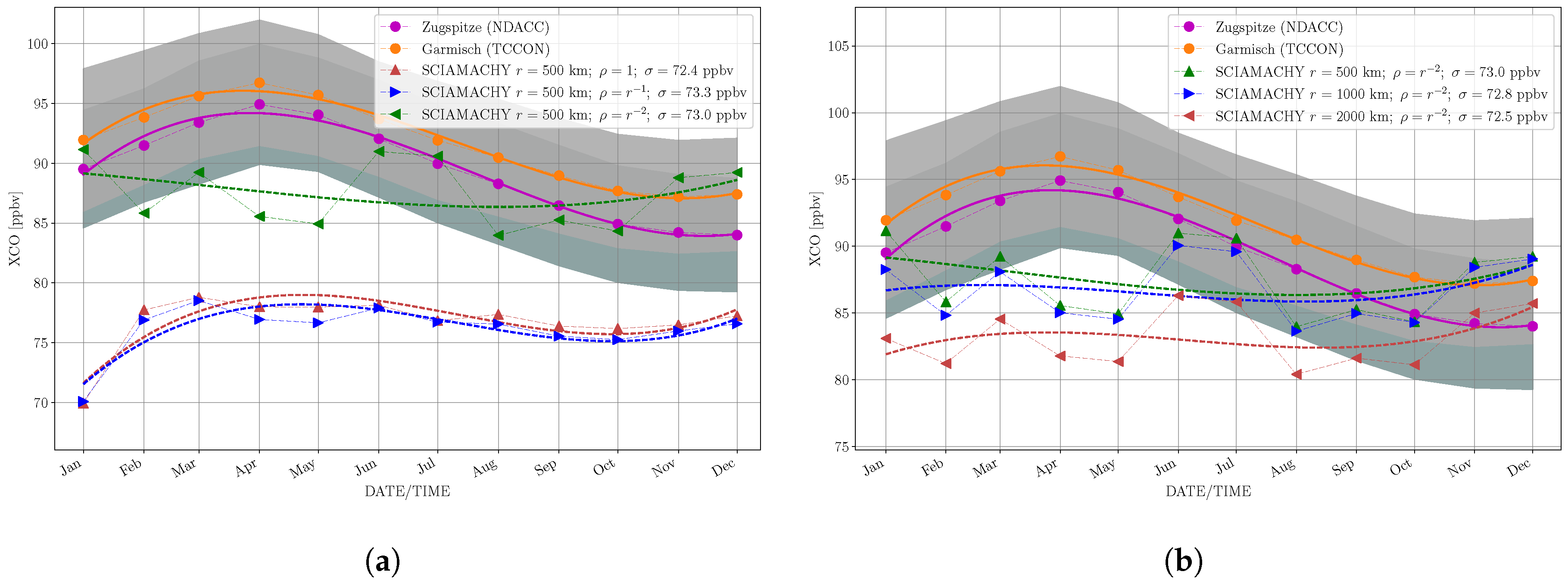
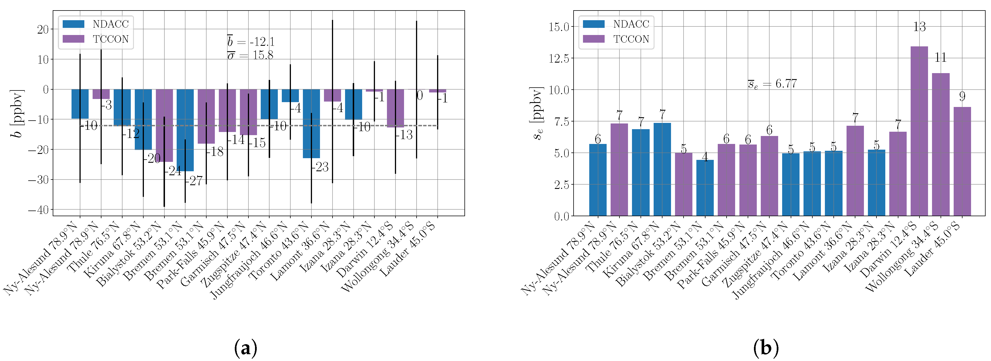
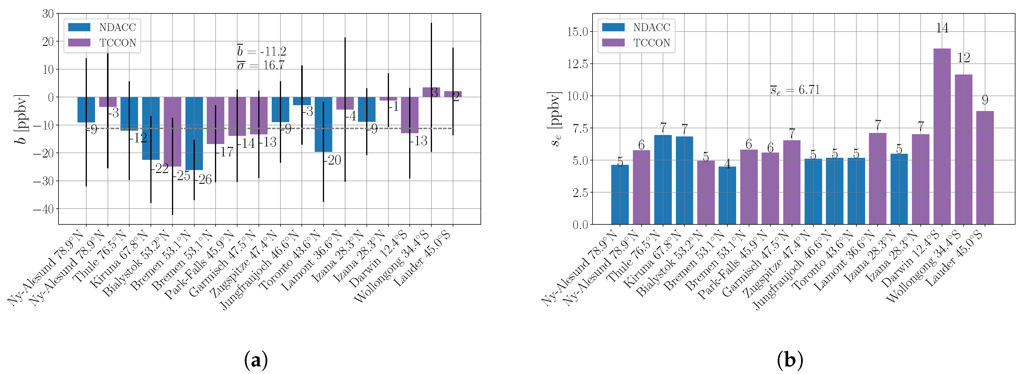
3.2.4. Multiannual Averages
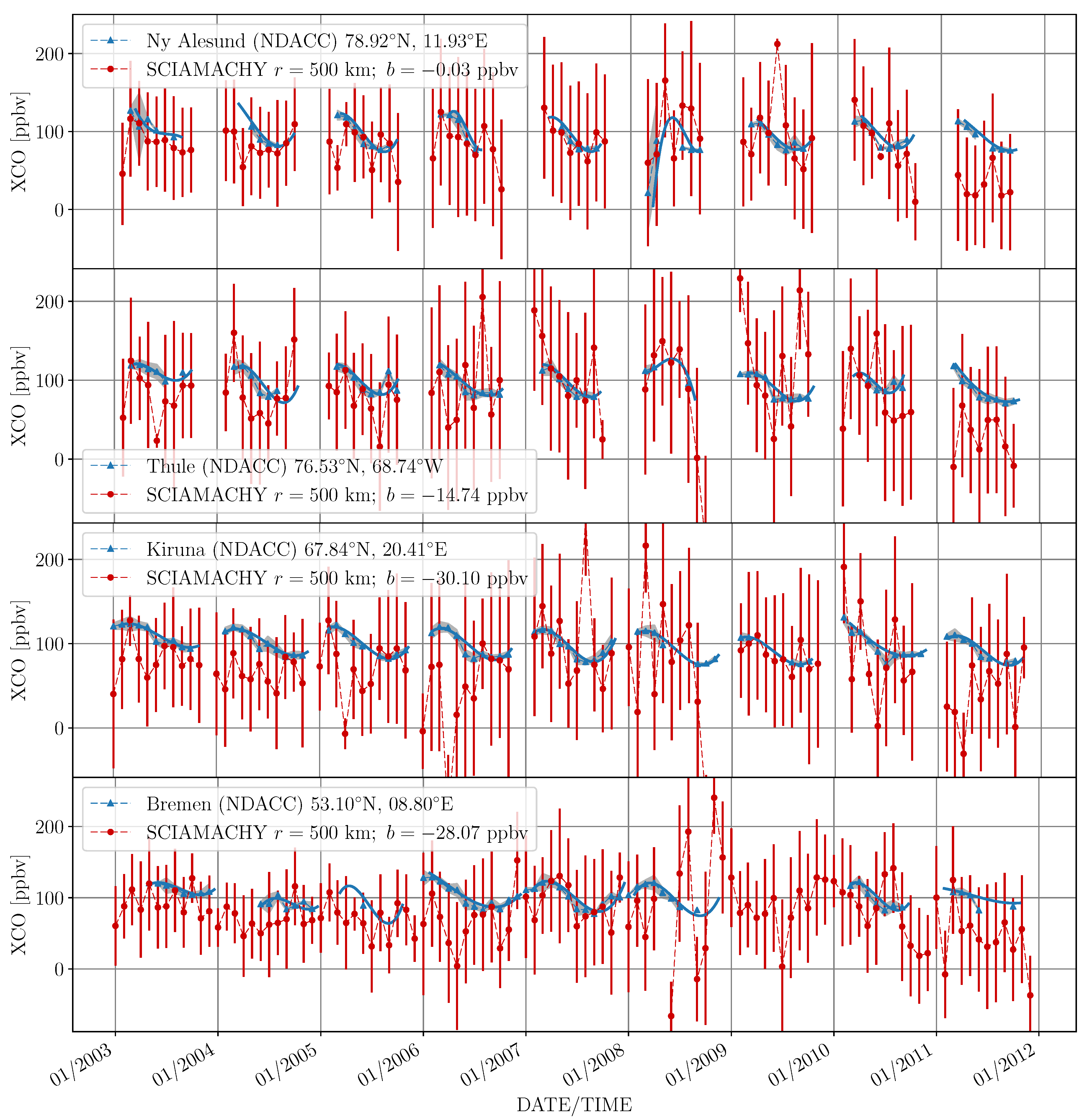
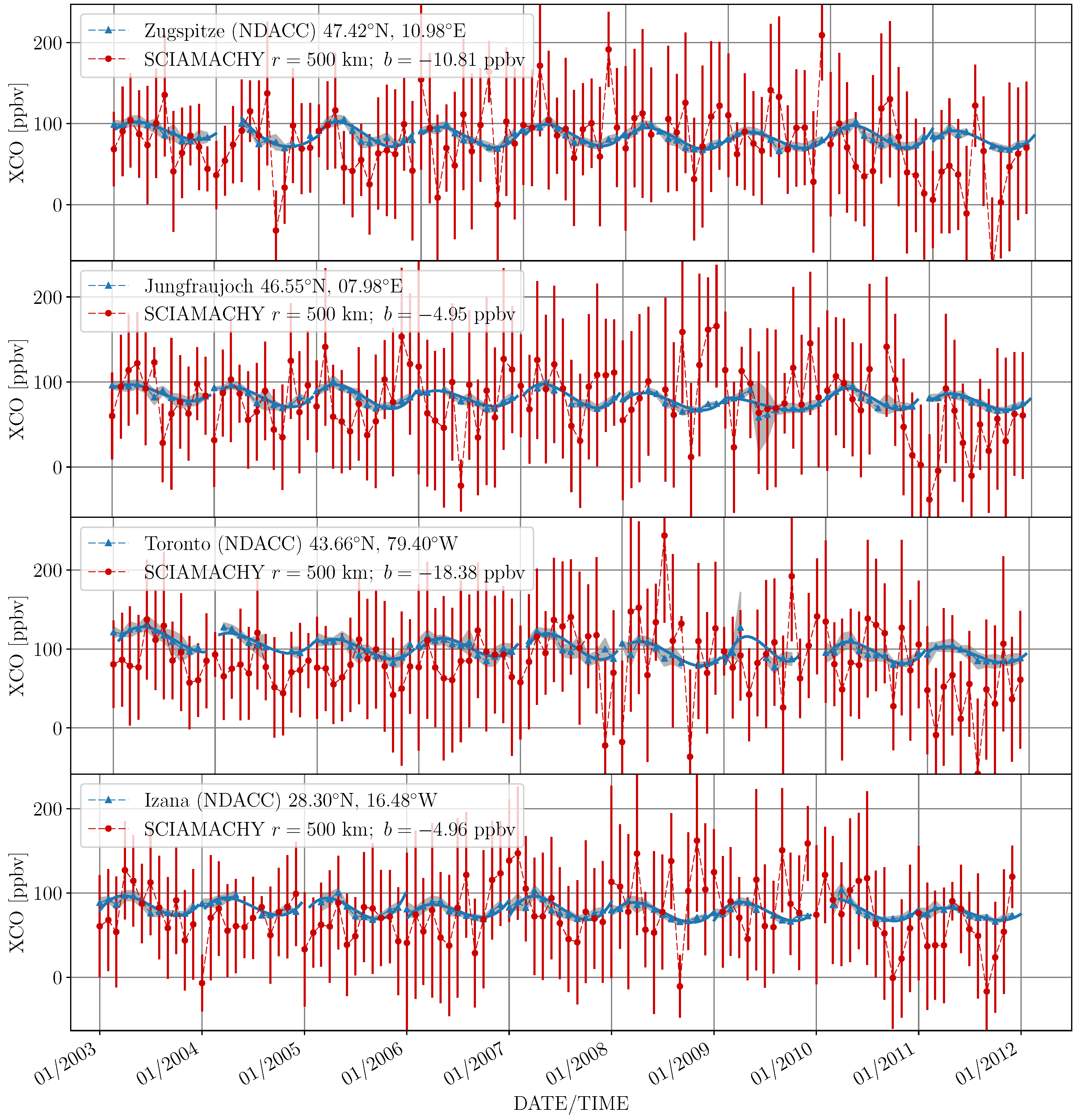
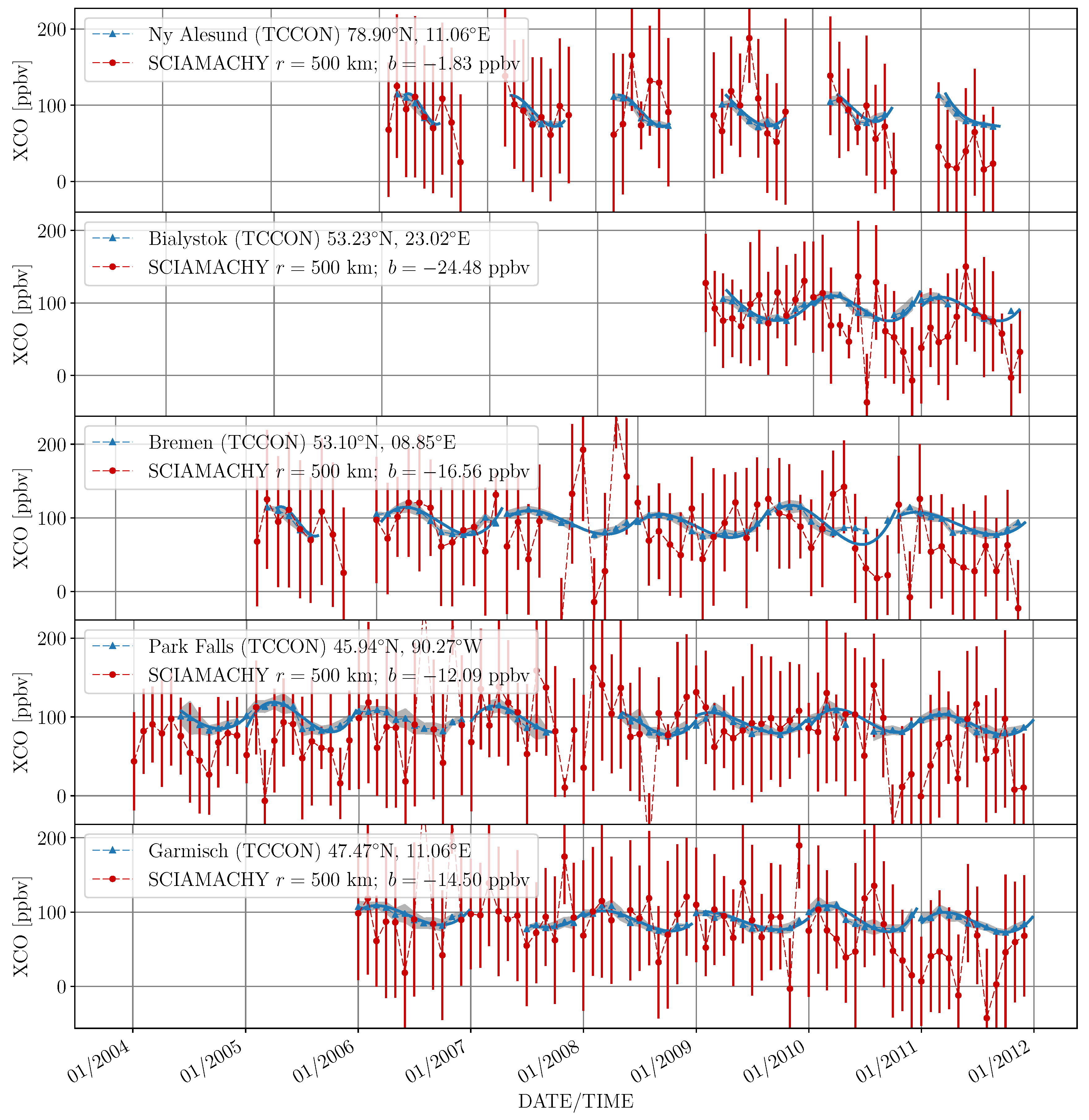
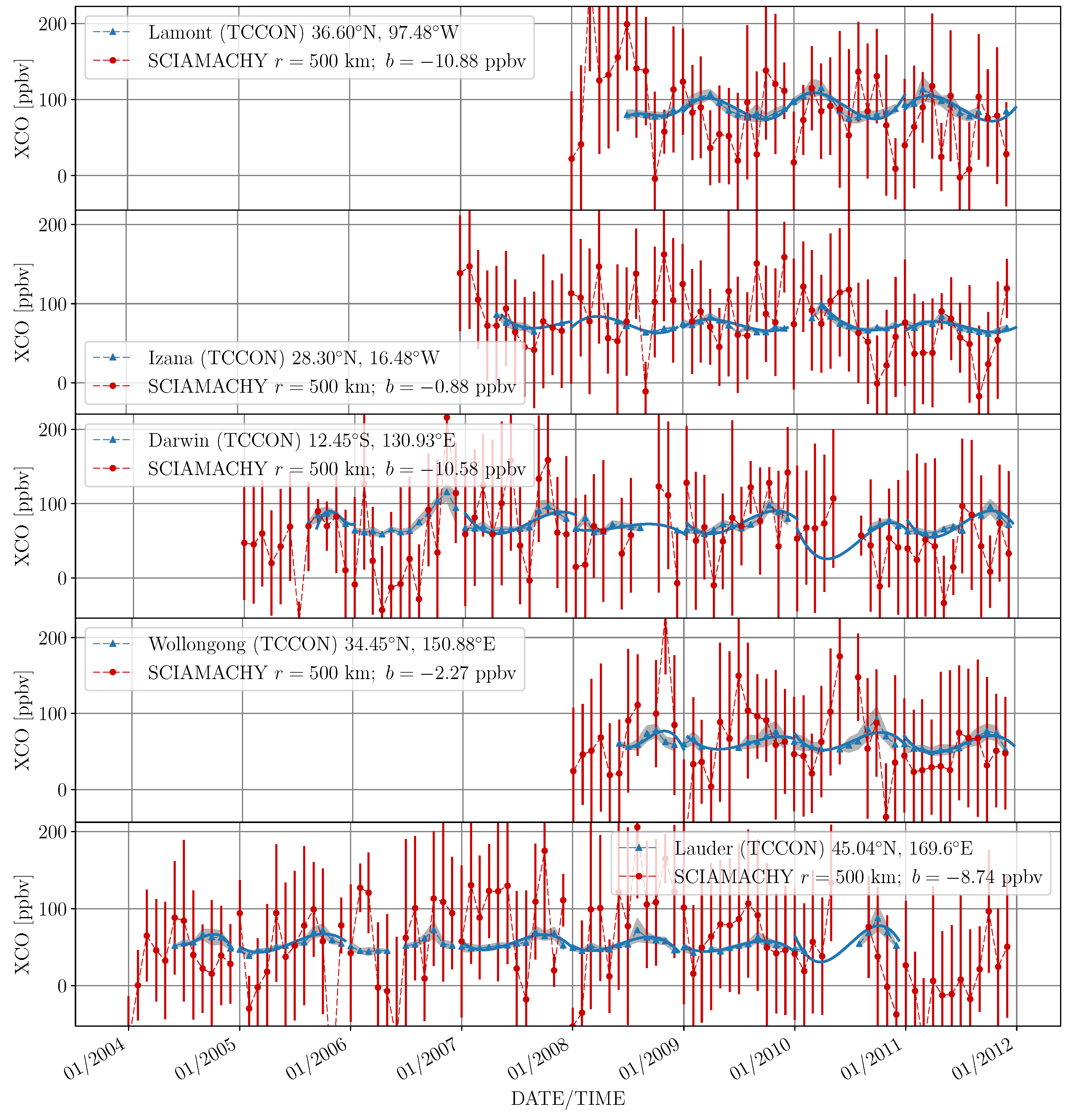
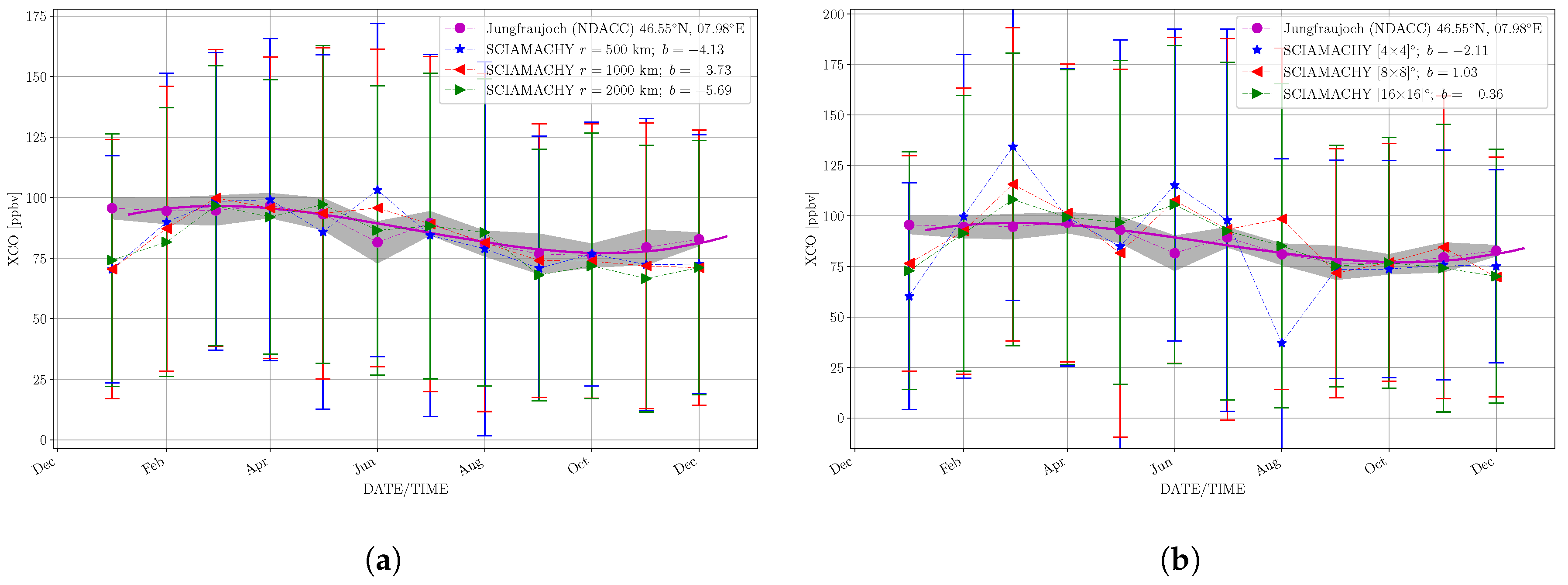
3.2.5. Time Series
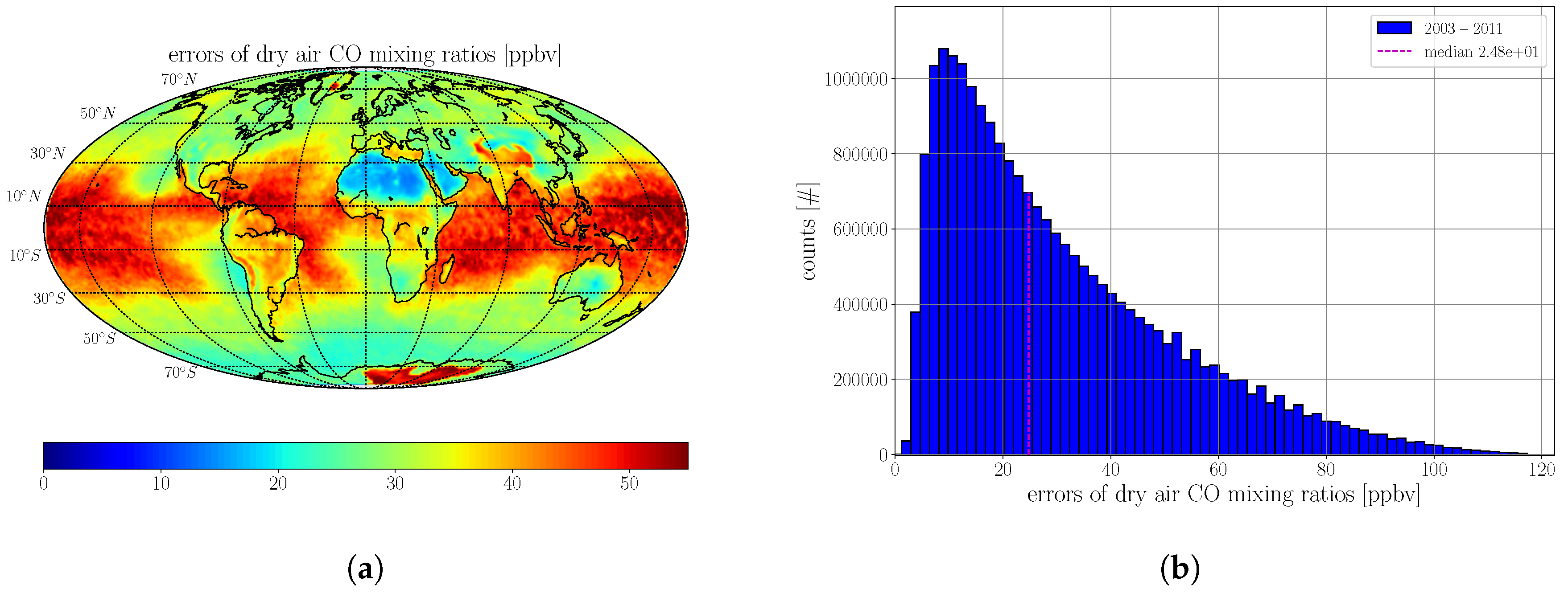
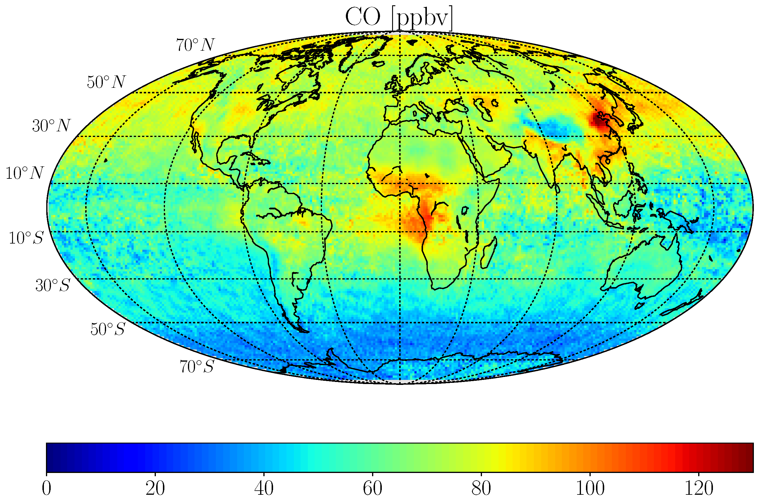
3.3. Mission Averaged Global CO
4. Discussion
4.1. Weighted Averages
4.2. Temporal Averages
4.3. Multiannual Averages
4.4. Spatio-Temporal Averages:
4.5. CO from TIR vs SWIR Observations
5. Conclusions
Supplementary Materials
Acknowledgments
Author Contributions
Conflicts of Interest
Abbreviations
| AIRS | Atmospheric Infrared Sounder |
| BIRRA | Beer InfraRed Retrieval Algorithm |
| CH4 | Methane |
| CMR | Column mixing ratio |
| CO | Carbon monoxide |
| CrIS | Cross-track Infrared Sounder |
| DOAS | Differential Optical Absorption Spectroscopy |
| ENVISAT | Environmental Satellite |
| FTIR | Fourier transform infrared |
| FTS | Fourier transform spectroscopy |
| G-B | Ground-based |
| GOMOS | Global Ozone Monitoring by Occultation of Stars |
| IASI | Infrared Atmospheric Sounding Interferometer |
| IMAP | Iterative Maximum A Posteriori |
| MIPAS | Michelson Interferometer for Passive Atmospheric Sounding |
| MOPITT | Measurement of Pollution in the Troposphere |
| NDACC | Network for the Detection of Atmospheric Composition Change |
| O2 | Oxygen |
| PPBV | Parts per billion in volume |
| S-B | Satellite-based |
| S5P | Sentinel-5 Precursor |
| SCIAMACHY | Scanning Imaging Absorption Spectrometer for Atmospheric Chartography |
| SICOR | Shortwave infrared CO retrieval |
| SWIR | Short-wave infrared |
| TCCON | Total Carbon Column Observing Network |
| TES | Tropospheric emission spectrometer |
| TIR | Thermal infrared |
| TROPOMI | Tropospheric Monitoring Instrument |
| VMR | Volume mixing ratio |
| WFM | Weighting function modified |
| XCO | Dry-air average column mixing ratio |
Appendix A. NDACC Data Providers

| NDACC Site | Coorperating Institutions |
|---|---|
| Bremen | Institute of Environmental Physics, University of Bremen, Germany |
| Garmisch | Institute for Meteorology and Climate Research, Karlsruhe Institute of Technology, Gemany |
| Izana | Izana Atmospheric Research Center, AEMET- Meteorological State Agency, Spain |
| Jungfraujoch | Universtiy of Liége, Belgium |
| Kiruna | Institute of Space Physics, Sweden |
| Ny-Alesund | Institute of Environmental Physics, University of Bremen, Germany |
| Alfred Wegener Institute for Polar and Marine Research, Germany | |
| Thule | Danish Climate Center, Danish Meteorological Institute Copenhagen, Denmark |
| Toronto | Department of Physics, University of Toronto, Canada |
Appendix B. TCCON Data Providers
| TCCON Site | Reference |
|---|---|
| Bialystok | Deutscher et al. [56] |
| Bremen | Notholt et al. [57] |
| Darwin | Griffith et al. [58] |
| Garmisch | Sussmann and Rettinger [59] |
| Izana | Blumenstock et al. [60] |
| Lamont | Wennberg et al. [61] |
| Lauder | Sherlock et al. [62] |
| Ny-Alesund | Notholt et al. [63] |
| Park-Falls | Wennberg et al. [64] |
| Wollongong | Griffith et al. [65] |
References
- ESA. ESA Declares End of Mission for ENVISAT. 2012. Available online: https://earth.esa.int/web/guest/missions/esa-operational-eo-missions/envisat (accessed on 15 January 2018).
- Gottwald, M.; Bovensmann, H. (Eds.) SCIAMACHY—Exploring the Changing Earth’s Atmosphere; Springer: Dordrecht, The Netherlands, 2011. [Google Scholar]
- Gloudemans, A.; Schrijver, H.; Kleipool, Q.; van den Broek, M.; Straume, A.; Lichtenberg, G.; van Hees, R.; Aben, I.; Meirink, J. The impact of SCIAMACHY near-infrared instrument calibration on CH4 and CO total columns. Atmos. Chem. Phys. 2005, 5, 2369–2383. [Google Scholar] [CrossRef] [Green Version]
- Lichtenberg, G.; Gimeno Garcia, S.; Schreier, F.; Slijkhuis, S.; Snel, R.; Bovensmann, H. Impact of Level 1 Quality on SCIAMACHY Level 2 Retrieval. In Proceedings of the 38th COSPAR Scientific Assembly, Bremen, Germany, 18–25 July 2010. [Google Scholar]
- Buchwitz, M.; de Beek, R.; Bramstedt, K.; Noël, S.; Bovensmann, H.; Burrows, J.P. Global carbon monoxide as retrieved from SCIAMACHY by WFM-DOAS. Atmos. Chem. Phys. 2004, 4, 1945–1960. [Google Scholar] [CrossRef]
- Buchwitz, M.; de Beek, R.; Noël, S.; Burrows, J.P.; Bovensmann, H.; Bremer, H.; Bergamaschi, P.; Körner, S.; Heimann, M. Carbon monoxide, methane and carbon dioxide columns retrieved from SCIAMACHY by WFM-DOAS: year 2003 initial data set. Atmos. Chem. Phys. 2005, 5, 3313–3329. [Google Scholar] [CrossRef]
- Frankenberg, C.; Platt, U.; Wagner, T. Retrieval of CO from SCIAMACHY onboard ENVISAT: Detection of strongly polluted areas and seasonal patterns in global CO abundances. Atmos. Chem. Phys. 2005, 5, 1639–1644. [Google Scholar] [CrossRef]
- Gimeno García, S.; Schreier, F.; Lichtenberg, G.; Slijkhuis, S. Near infrared nadir retrieval of vertical column densities: methodology and application to SCIAMACHY. Atmos. Meas. Tech. 2011, 4, 2633–2657. [Google Scholar] [CrossRef] [Green Version]
- Borsdorff, T.; Tol, P.; Williams, J.E.; de Laat, J.; aan de Brugh, J.; Nédélec, P.; Aben, I.; Landgraf, J. Carbon monoxide total columns from SCIAMACHY 2.3 μm atmospheric reflectance measurements: Towards a full-mission data product (2003–2012). Atmos. Meas. Tech. 2016, 9, 227–248. [Google Scholar] [CrossRef]
- Borsdorff, T.; aan de Brugh, J.; Hu, H.; Nédélec, P.; Aben, I.; Landgraf, J. Carbon monoxide column retrieval for clear-sky and cloudy atmospheres: a full-mission data set from SCIAMACHY 2.3 μm reflectance measurements. Atmos. Meas. Tech. 2017, 10, 1769–1782. [Google Scholar] [CrossRef]
- Clerbaux, C.; Boynard, A.; Clarisse, L.; George, M.; Hadji-Lazaro, J.; Herbin, H.; Hurtmans, D.; Pommier, M.; Razavi, A.; Turquety, S.; et al. Monitoring of atmospheric composition using the thermal infrared IASI/MetOp sounder. Atmos. Chem. Phys. 2009, 9, 6041–6054. [Google Scholar] [CrossRef] [Green Version]
- Fischer, H.; Birk, M.; Blom, C.; Carli, B.; Carlotti, M.; von Clarmann, T.; Delbouille, L.; Dudhia, A.; Ehhalt, D.; Endemann, M.; et al. MIPAS: an instrument for atmospheric and climate research. Atmos. Chem. Phys. 2008, 8, 2151–2188. [Google Scholar] [CrossRef]
- Bernath, P.; McElroy, C.T.; Abrams, M.C.; Boone, C.D.; Butler, M.; Camy-Peyret, C.; Carleer, M.; Clerbaux, C.; Coheur, P.F.; Colin, R.; et al. Atmospheric Chemistry Experiment (ACE): Mission overview. Geophys. Res. Lett. 2005, 32, L15S01. [Google Scholar] [CrossRef]
- Kuze, A.; Suto, H.; Nakajima, M.; Hamazaki, T. Thermal and near infrared sensor for carbon observation Fourier-transform spectrometer on the Greenhouse Gases Observing Satellite for greenhouse gases monitoring. Appl. Opt. 2009, 48, 6716–6733. [Google Scholar] [CrossRef] [PubMed]
- Wunch, D.; Toon, G.C.; Blavier, J.F.L.; Washenfelder, R.A.; Notholt, J.; Connor, B.J.; Griffith, D.W.T.; Sherlock, V.; Wennberg, P.O. The Total Carbon Column Observing Network. Philos. Trans. R. Soc. A 2011, 369, 2087–2112. [Google Scholar] [CrossRef] [PubMed]
- Feist, D. Global FTS-Network. 2015. Available online: https://oc.bgc-jena.mpg.de (accessed on 20 June 2016).
- Warnek, T.; Notholt, J.; Chen, H. Validation and Calibration of Greenhouse-Gas Satellite Observations by Ground-Based Remote Sensing Measurements; University of Bremen: Bibliothekstraße, Bremen, 2015. [Google Scholar]
- TCCON. Total Carbon Column Observing Network—Wiki. 2018. Available online: https://tccon-wiki.caltech.edu/Network_Policy/Data_Use_Policy/Data_Description#Measurement_precision_(repeatability) (accessed on 11 January 2018).
- Einarsson, B. (Ed.) Accuracy and Reliability in Scientific Computing; SIAM: Philadelphia, PA, USA, 2005. [Google Scholar]
- Verhoelst, T.; Granville, J.; Hendrick, F.; Köhler, U.; Lerot, C.; Pommereau, J.P.; Redondas, A.; Van Roozendael, M.; Lambert, J.C. Metrology of ground-based satellite validation: co-location mismatch and smoothing issues of total ozone comparisons. Atmos. Meas. Tech. 2015, 8, 5039–5062. [Google Scholar] [CrossRef] [Green Version]
- De Laat, A.T.J.; Gloudemans, A.M.S.; Schrijver, H.; Aben, I.; Nagahama, Y.; Suzuki, K.; Mahieu, E.; Jones, N.B.; Paton-Walsh, C.; Deutscher, N.M.; et al. Validation of five years (2003–2007) of SCIAMACHY CO total column measurements using ground-based spectrometer observations. Atmos. Meas. Tech. 2010, 3, 1457–1471. [Google Scholar] [CrossRef] [Green Version]
- De Laat, A.; Gloudemans, A.; Schrijver, H.; van den Broek, M.; Meirink, J.; Aben, I.; Krol, M. Quantitative analysis of SCIAMACHY carbon monoxide total column measurements. Geophys. Res. Lett. 2006, 33, L07807. [Google Scholar] [CrossRef]
- Sussmann, R.; Buchwitz, M. Initial validation of ENVISAT/SCIAMACHY columnar CO by FTIR profile retrievals at the Ground-Truthing Station Zugspitze. Atmos. Chem. Phys. 2005, 5, 1497–1503. [Google Scholar] [CrossRef]
- Sussmann, R.; Stremme, W.; Buchwitz, M.; de Beek, R. Validation of ENVISAT/SCIAMACHY columnar methane by solar FTIR spectrometry at the Ground-Truthing Station Zugspitze. Atmos. Chem. Phys. 2005, 5, 2419–2429. [Google Scholar] [CrossRef]
- Dils, B.; De Maziere, M.; Muller, J.; Blumenstock, T.; Buchwitz, M.; de Beek, R.; Demoulin, P.; Duchatelet, P.; Fast, H.; Frankenberg, C.; et al. Comparisons between SCIAMACHY and ground-based FTIR data for total columns of CO, CH4, CO2 and N2O. Atmos. Chem. Phys. 2006, 6, 1953–1976. [Google Scholar] [CrossRef]
- Schneising, O.; Bergamaschi, P.; Bovensmann, H.; Buchwitz, M.; Burrows, J.P.; Deutscher, N.M.; Griffith, D.W.T.; Heymann, J.; Macatangay, R.; Messerschmidt, J.; et al. Atmospheric greenhouse gases retrieved from SCIAMACHY: Comparison to ground-based FTS measurements and model results. Atmos. Chem. Phys. 2012, 12, 1527–1540. [Google Scholar] [CrossRef] [Green Version]
- Meier, A. Spectroscopic Atlas of Atmospheric Microwindows in the Middle Infrared; IRF Technical Report; IRF Institute för Rymdfysik: Kiruna, Sweden, 2004. [Google Scholar]
- Kiel, M.; Wunch, D.; Wennberg, P.O.; Toon, G.C.; Hase, F.; Blumenstock, T. Improved retrieval of gas abundances from near-infrared solar FTIR spectra measured at the Karlsruhe TCCON station. Atmos. Meas. Tech. 2016, 9, 669–682. [Google Scholar] [CrossRef]
- Wunch, D.; Toon, G.C.; Sherlock, V.; Deutscher, N.M.; Liu, C.; Feist, D.G.; Wennberg, P.O. The Total Carbon Column Observing Network’s GGG2014 Data Version; Technical Report; Carbon Dioxide Information Analysis Center, Oak Ridge National Laboratory: Oak Ridge, TN, USA, 2015.
- Schreier, F.; Gimeno García, S.; Hedelt, P.; Hess, M.; Mendrok, J.; Vasquez, M.; Xu, J. GARLIC—A General Purpose Atmospheric Radiative Transfer Line-by-Line Infrared-Microwave Code: Implementation and Evaluation. J. Quant. Spectrosc. Radiat. Transf. 2014, 137, 29–50. [Google Scholar] [CrossRef]
- Schreier, F.; Gimeno García, S.; Vasquez, M.; Xu, J. Algorithmic vs. finite difference Jacobians for infrared atmospheric radiative transfer. J. Quant. Spectrosc. Radiat. Transf. 2015, 164, 147–160. [Google Scholar] [CrossRef]
- Dennis, J., Jr.; Gay, D.; Welsch, R. Algorithm 573: NL2SOL—An Adaptive Nonlinear Least–Squares Algorithm. ACM Trans. Math. Softw. 1981, 7, 369–383. [Google Scholar] [CrossRef]
- Golub, G.; Pereyra, V. Separable nonlinear least squares: the variable projection method and its applications. Inverse Probl. 2003, 19, R1–R26. [Google Scholar] [CrossRef]
- Anderson, G.; Clough, S.; Kneizys, F.; Chetwynd, J.; Shettle, E. AFGL Atmospheric Constituent Profiles (0–120 km); Technical Report TR-86-0110; AFGL: Hanscom AFB, MA, USA, 1986. [Google Scholar]
- Gloudemans, A.; de Laat, A.; Schrijver, H.; Aben, I.; Meirink, J.; van der Werf, G. SCIAMACHY CO over land and oceans: 2003–2007 interannual variability. Atmos. Chem. Phys. 2009, 9, 3799–3813. [Google Scholar] [CrossRef]
- Buschmann, M.; Deutscher, N.M.; Sherlock, V.; Palm, M.; Warneke, T.; Notholt, J. Retrieval of xCO2 from ground-based mid-infrared (NDACC) solar absorption spectra and comparison to TCCON. Atmos. Meas. Tech. 2016, 9, 577–585. [Google Scholar] [CrossRef]
- Ostler, A.; Sussmann, R.; Rettinger, M.; Deutscher, N.M.; Dohe, S.; Hase, F.; Jones, N.; Palm, M.; Sinnhuber, B.M. Multistation intercomparison of column-averaged methane from NDACC and TCCON: Impact of dynamical variability. Atmos. Meas. Tech. 2014, 7, 4081–4101. [Google Scholar] [CrossRef]
- Filipiak, M.; Harwood, R.; Jiang, J.; Li, Q.; Livesey, N.; Manney, G.; Read, W.; Schwartz, M.; Waters, J.; Wu, D. Carbon Monoxide Measured by the EOS Microwave Limb Sounder on Aura: First Results. Geophys. Res. Lett. 2005, 32, L14825. [Google Scholar] [CrossRef]
- Pumphrey, H.; Filipiak, M.; Livesey, N.; Schwartz, M.; Boone, C.; Walker, K.; Bernath, P.; Ricaud, P.; Barret, B.; Clerbaux, C.; et al. Validation of middle-atmosphere carbon monoxide retrievals from the Microwave Limb Sounder on Aura. J. Geophys. Res. 2007, 112, D24S38. [Google Scholar] [CrossRef]
- Dupuy, E.; Urban, J.; Ricaud, P.; Le Flochmoën, E.; Lautié, N.; Murtagh, D.; De La Noë, J.; El Amraoui, L.; Eriksson, P.; Forkman, P.; et al. Strato-mesospheric measurements of carbon monoxide with the Odin Sub-Millimetre Radiometer: Retrieval and first results. Geophys. Res. Lett. 2004, 31, L20101. [Google Scholar] [CrossRef]
- McMillan, W.W.; Barnet, C.; Strow, L.; Chahine, M.T.; McCourt, M.L.; Warner, J.X.; Novelli, P.C.; Korontzi, S.; Maddy, E.S.; Datta, S. Daily global maps of carbon monoxide from NASA’s Atmospheric Infrared Sounder. Geophys. Res. Lett. 2005, 32, L11801. [Google Scholar] [CrossRef]
- Gambacorta, A.; Barnet, C.; Wolf, W.; King, T.; Maddy, E.; Strow, L.; Xiong, X.; Nalli, N.; Goldberg, M. An Experiment Using High Spectral Resolution CrIS Measurements for Atmospheric Trace Gases: Carbon Monoxide Retrieval Impact Study. IEEE Geosci. Remote Sens. Lett. 2014, 11, 1639–1643. [Google Scholar] [CrossRef]
- Fu, D.; Bowman, K.W.; Worden, H.M.; Natraj, V.; Worden, J.R.; Yu, S.; Veefkind, P.; Aben, I.; Landgraf, J.; Strow, L.; et al. High-resolution tropospheric carbon monoxide profiles retrieved from CrIS and TROPOMI. Atmos. Meas. Tech. 2016, 9, 2567–2579. [Google Scholar] [CrossRef]
- George, M.; Clerbaux, C.; Hurtmans, D.; Turquety, S.; Coheur, P.F.; Pommier, M.; Hadji-Lazaro, J.; Edwards, D.P.; Worden, H.; Luo, M.; et al. Carbon monoxide distributions from the IASI/METOP mission: evaluation with other space-borne remote sensors. Atmos. Chem. Phys. 2009, 9, 8317–8330. [Google Scholar] [CrossRef] [Green Version]
- Fortems-Cheiney, A.; Chevallier, F.; Pison, I.; Bousquet, P.; Carouge, C.; Clerbaux, C.; Coheur, P.F.; George, M.; Hurtmans, D.; Szopa, S. On the capability of IASI measurements to inform about CO surface emissions. Atmos. Chem. Phys. 2009, 9, 8735–8743. [Google Scholar] [CrossRef] [Green Version]
- Illingworth, S.; Remedios, J.; Boesch, H.; Moore, D.; Sembhi, H.; Dudhia, A.; Walker, J. ULIRS, an optimal estimation retrieval scheme for carbon monoxide using IASI spectral radiances: sensitivity analysis, error budget and simulations. Atmos. Meas. Tech. 2011, 4, 269–288. [Google Scholar] [CrossRef] [Green Version]
- Deeter, M.N.; Emmons, L.K.; Francis, G.L.; Edwards, D.P.; Gille, J.C.; Warner, J.X.; Khattatov, B.; Ziskin, D.; Lamarque, J.F.; Ho, S.P.; et al. Operational carbon monoxide retrieval algorithm and selected results for the MOPITT instrument. J. Geophys. Res. 2003, 108. [Google Scholar] [CrossRef]
- Rinsland, C.; Luo, M.; Logan, J.; Beer, R.; Worden, H.; Worden, J.; Bowman, K.; Kulawik, S.; Rider, D.; Osterman, G.; et al. Nadir Measurements of Carbon Monoxide Distributions by the Tropospheric Emission Spectrometer onboard the Aura Spacecraft: Overview of Analysis Approach and Examples of Initial Results. Geophys. Res. Lett. 2006, 33, L22806. [Google Scholar] [CrossRef]
- Worden, H.; Deeter, M.; Edwards, D.; Gille, J.; Drummond, J.; Nédélec, P. Observations of near-surface carbon monoxide from space using MOPITT multispectral retrievals. J. Geophys. Res. 2010, 115, D16314. [Google Scholar] [CrossRef]
- Emmons, L.; Pfister, G.; Edwards, D.; Gille, J.; Sachse, G.; Blake, D.; Wofsy, S.; Gerbig, C.; Matross, D.; Nedelec, P. Measurements of Pollution in the Troposphere (MOPITT) validation exercises during summer 2004 field campaigns over North America. J. Geophys. Res. 2007, 112, D12S02. [Google Scholar] [CrossRef]
- De Laat, A.; Gloudemans, A.; Aben, I.; Krol, M.; Meirink, J.; van der Werf, G.; Schrijver, H. Scanning Imaging Absorption Spectrometer for Atmospheric Chartography carbon monoxide total columns: Statistical evaluation and comparison with chemistry transport model results. J. Geophys. Res. 2007, 112, D12310. [Google Scholar] [CrossRef]
- Kopacz, M.; Jacob, D.J.; Fisher, J.A.; Logan, J.A.; Zhang, L.; Megretskaia, I.A.; Yantosca, R.M.; Singh, K.; Henze, D.K.; Burrows, J.P.; et al. Global estimates of CO sources with high resolution by adjoint inversion of multiple satellite datasets (MOPITT, AIRS, SCIAMACHY, TES). Atmos. Chem. Phys. 2010, 10, 855–876. [Google Scholar] [CrossRef]
- Tangborn, A.; Stajner, I.; Buchwitz, M.; Khlystova, I.; Pawson, S.; Burrows, J.; Hudman, R.; Nedelec, P. Assimilation of SCIAMACHY total column CO observations: Global and regional analysis of data impact. J. Geophys. Res. 2009, 114, D07307. [Google Scholar] [CrossRef]
- Schreier, F.; Gimeno García, S.; Lichtenberg, G.; Hoffmann, P. Intercomparison of Carbon Monoxide Retrievals from SCIAMACHY and AIRS Nadir Observations. In Proceedings of the Atmospheric Science Conference, Barcelona, Spain, 7–11 September 2009; Volume SP-676. [Google Scholar]
- Landgraf, J.; aan de Brugh, J.; Scheepmaker, R.; Borsdorff, T.; Hu, H.; Houweling, S.; Butz, A.; Aben, I.; Hasekamp, O. Carbon monoxide total column retrievals from TROPOMI shortwave infrared measurements. Atmos. Meas. Tech. 2016, 9, 4955–4975. [Google Scholar] [CrossRef]
- Deutscher, N.M.; Notholt, J.; Messerschmidt, J.; Weinzierl, C.; Warneke, T.; Petri, C.; Grupe, P.; Katrynski, K. TCCON Data from Bialystok (PL), Release GGG2014.R1; TCCON Data Archive; CaltechDATA, California Institute of Technology: Pasadena, CA, USA, 2015. [Google Scholar] [CrossRef]
- Notholt, J.; Petri, C.; Warneke, T.; Deutscher, N.M.; Buschmann, M.; Weinzierl, C.; Macatangay, R.C.; Grupe, P. TCCON Data from Bremen (DE), Release GGG2014.R0; TCCON Data Archive; CaltechDATA, California Institute of Technology: Pasadena, CA, USA, 2014. [Google Scholar] [CrossRef]
- Griffith, D.W.T.; Deutscher, N.M.; Velazco, V.A.; Wennberg, P.O.; Yavin, Y.; Keppel-Aleks, G.; Washenfelder, R.; Toon, G.C.; Blavier, J.F.; Paton-Walsh, C.; et al. TCCON Data from Darwin (AU), Release GGG2014.R0; TCCON Data Archive; CaltechDATA, California Institute of Technology: Pasadena, CA, USA, 2014. [Google Scholar] [CrossRef]
- Sussmann, R.; Rettinger, M. TCCON Data from Garmisch (DE), Release GGG2014.R0; TCCON Data Archive; CaltechDATA, California Institute of Technology: Pasadena, CA, USA, 2014. [Google Scholar] [CrossRef]
- Blumenstock, T.; Hase, F.; Schneider, M.; Garcia, O.E.; Sepulveda, E. TCCON Data from Izana (ES), Release GGG2014.R0; TCCON Data Archive; CaltechDATA, California Institute of Technology: Pasadena, CA, USA, 2014. [Google Scholar] [CrossRef]
- Wennberg, P.O.; Wunch, D.; Roehl, C.; Blavier, J.F.; Toon, G.C.; Allen, N. TCCON Data from Lamont (US), Release GGG2014.R1; TCCON Data Archive; CaltechDATA, California Institute of Technology: Pasadena, CA, USA, 2016. [Google Scholar] [CrossRef]
- Sherlock, V.; Connor, B.; Robinson, J.; Shiona, H.; Smale, D.; Pollard, D. TCCON Data from Lauder (NZ), 120HR, Release GGG2014.R0; TCCON Data Archive; CaltechDATA, California Institute of Technology: Pasadena, CA, USA, 2014. [Google Scholar] [CrossRef]
- Notholt, J.; Warneke, T.; Petri, C.; Deutscher, N.M.; Weinzierl, C.; Palm, M.; Buschmann, M. TCCON Data from Ny Ålesund, Spitsbergen (NO), Release GGG2014.R0; TCCON Data Archive; CaltechDATA, California Institute of Technology: Pasadena, CA, USA, 2017. [Google Scholar] [CrossRef]
- Wennberg, P.O.; Roehl, C.; Wunch, D.; Toon, G.C.; Blavier, J.F.; Washenfelder, R.; Keppel-Aleks, G.; Allen, N.; Ayers, J. TCCON Data from Park Falls (US), Release GGG2014.R0; TCCON Data Archive; CaltechDATA, California Institute of Technology: Pasadena, CA, USA, 2014. [Google Scholar] [CrossRef]
- Griffith, D.W.T.; Velazco, V.A.; Deutscher, N.M.; Paton-Walsh, C.; Jones, N.B.; Wilson, S.R.; Macatangay, R.C.; Kettlewell, G.C.; Buchholz, R.R.; Riggenbach, M. TCCON Data from Wollongong (AU), Release GGG2014.R0; TCCON Data Archive; CaltechDATA, California Institute of Technology: Pasadena, CA, USA, 2014. [Google Scholar] [CrossRef]


| Stations | Lat N [] | Lon E [] | Altitude [m] | NDACC (years) | TCCON (years) |
|---|---|---|---|---|---|
| Bialystock | 53.23 | 23.03 | 160 | - | 2009–2011 |
| Bremen | 53.10 | 8.85 | 30 | 2003–2011 | 2005–2011 |
| Darwin | −12.42 | 130.89 | 30 | - | 2005–2011 |
| Garmisch | 47.48 | 11.06 | 743 | - | 2007–2011 |
| Izana | 28.30 | −16.48 | 2367 | 2003–2011 | 2007–2011 |
| Jungfraujoch | 46.55 | 7.98 | 3580 | 2003–2011 | - |
| Kiruna | 67.84 | 20.40 | 420 | 2003–2011 | - |
| Lamont | 36.60 | −97.49 | 320 | - | 2008–2011 |
| Lauder | −45.04 | 169.68 | 370 | - | 2004–2010 |
| Ny Alesund | 78.92 | 11.93 | 15 | 2003–2011 | 2005–2011 |
| Parkfalls | 45.95 | −90.27 | 442 | - | 2004–2011 |
| Thule | 76.52 | −68.77 | 220 | 2003–2011 | - |
| Toronto | 43.66 | −79.40 | 174 | 2003–2011 | - |
| Wollongong | −34.41 | 150.88 | 30 | - | 2008–2011 |
| Zugspitze | 47.42 | 10.98 | 2964 | 2003–2011 | - |
| Algorithm | Wavenumber [cm] | Interfering Species |
|---|---|---|
| SFIT | 2057.8575 | NO, COF ... |
| (NDACC) | 2069.6559 | NO, COF ... |
| 2111.5430 | OCS, N ... | |
| 2158.2997 | OCS, N ... | |
| GFIT | 4208.70–4257.30 | HO, CH |
| (TCCON) | 4262.00–4318.80 | HO, CH |
| BIRRA | 4280.00–4305.00 | HO, CH |
| (SCIAMACHY) |
| ppbv | 1 | r | r | |||
|---|---|---|---|---|---|---|
| NDACC | −14.3 | 5.5 | −13.8 | 5.4 | −14.4 | 5.1 |
| TCCON | −8.1 | 7.7 | −7.4 | 7.9 | −9.1 | 7.1 |
© 2018 by the authors. Licensee MDPI, Basel, Switzerland. This article is an open access article distributed under the terms and conditions of the Creative Commons Attribution (CC BY) license (http://creativecommons.org/licenses/by/4.0/).
Share and Cite
Hochstaffl, P.; Schreier, F.; Lichtenberg, G.; Gimeno García, S. Validation of Carbon Monoxide Total Column Retrievals from SCIAMACHY Observations with NDACC/TCCON Ground-Based Measurements. Remote Sens. 2018, 10, 223. https://doi.org/10.3390/rs10020223
Hochstaffl P, Schreier F, Lichtenberg G, Gimeno García S. Validation of Carbon Monoxide Total Column Retrievals from SCIAMACHY Observations with NDACC/TCCON Ground-Based Measurements. Remote Sensing. 2018; 10(2):223. https://doi.org/10.3390/rs10020223
Chicago/Turabian StyleHochstaffl, Philipp, Franz Schreier, Günter Lichtenberg, and Sebastian Gimeno García. 2018. "Validation of Carbon Monoxide Total Column Retrievals from SCIAMACHY Observations with NDACC/TCCON Ground-Based Measurements" Remote Sensing 10, no. 2: 223. https://doi.org/10.3390/rs10020223