Evaluating the Performance of the SCOPE Model in Simulating Canopy Solar-Induced Chlorophyll Fluorescence


1
Key Laboratory of Digital Earth Science, Institute of Remote Sensing and Digital Earth, Chinese Academy of Sciences, Beijing 100094, China
2
College of Resources and Environment, University of Chinese Academy of Sciences, Beijing 100049, China
*
Author to whom correspondence should be addressed.
Remote Sens. 2018, 10(2), 250; https://doi.org/10.3390/rs10020250
Submission received: 15 December 2017
/
Revised: 2 February 2018
/
Accepted: 4 February 2018
/
Published: 6 February 2018
(This article belongs to the Special Issue Advances in Quantitative Remote Sensing in China – In Memory of Prof. Xiaowen Li)
Abstract
:The SCOPE (soil canopy observation of photochemistry and energy fluxes) model has been widely used to interpret solar-induced chlorophyll fluorescence (SIF) and investigate the SIF-photosynthesis links at different temporal and spatial scales in recent years. In the SCOPE model, the fluorescence quantum efficiency in dark-adapted conditions (FQE) for Photosystem II (fqe2) and Photosystem I (fqe1) were two key parameters of SIF emission, which have always been parameterized as fixed values derived from laboratory measurements. To date, only a few studies have focused on evaluating the SCOPE model for SIF interpretation, and the variation of FQE values in the field remains controversial. In this study, the accuracy of the SCOPE model to simulate the canopy SIF was investigated using diurnal experiments on winter wheat. First, ten diurnal experiments were conducted on winter wheat, and the canopy SIF emissions and the SCOPE model’s input parameters were directly measured or indirectly retrieved from the spectral radiances, gross primary productivity (GPP) data, and meteorological records. Second, the SCOPE-simulated SIF emissions with fixed FQE values were evaluated using the observed canopy SIF data. The results show that the SCOPE model can reliably interpret the diurnal cycles of SIF variation and provide acceptable results of SIF simulations at the O2-B (SIFB) and O2-A (SIFA) bands with RRMSEs of 24.35% and 23.67%, respectively. However, the SCOPE-simulated SIFB and SIFA still contained large systematical deviations at some growth stages of wheat, and the seasonal cycles of the ratio between SIFB and SIFA (SIFA/SIFB) cannot be credibly reproduced. Finally, the SCOPE-simulated SIF emissions with variable FQE values were evaluated using the observed canopy SIF data. The simulating accuracy of SIFB and SIFA can be improved greatly using variable FQE values, and the SCOPE simulations track well with the seasonal SIFA/SIFB values with an RRMSE of 20.63%. The results indicated a clear seasonal pattern of FQE values for unbiased SIF simulation: from the erecting to the flowering stage of wheat, the ratio of fqe1 to fqe2 (fqe1/fqe2) gradually increased from 0.05–0.1 to 0.3–0.5, while the fqe2 value decreased from 0.013 to 0.007. Our quantitative results of the model assessment and the FQE adjustment support the use of the SCOPE model as a powerful tool for interpreting the SIF emissions and can serve as a significant reference for future applications of the SCOPE model.
1. Introduction
Solar-induced chlorophyll fluorescence (SIF) refers to the emission of red and far-red light from chlorophyll during the absorption of photosynthetically active radiation under natural sunlight. The SIF spectrum is a continuous broadband spectrum that covers the approximately spectral range of 650–850 nm. Its spectral shape is characterized by one peak at around 685 nm and another at around 740 nm [1,2]. The emitted SIF is the sum of the chlorophyll fluorescence of photosystem I (PSI) and photosystem II (PSII). PSII contributes to the SIF emission in both the red and far-red spectral regions, whereas PSI contributes to the SIF emission only in the far-red region [3]. As a result, the intensity and shape of the SIF spectrum can reflect the amount of energy absorbed by PSII and PSI [4,5]. In addition, several studies have determined the physics-physiology mechanism connecting function of the photosynthetic apparatus with chlorophyll fluorescence from active florescence induction measurement and demonstrated that the fluorescence signal can be a reliable and observable indicator of the plant’s photosynthetic status [4,5,6]. To date, extensive SIF-photosynthesis research has focused on investigating the empirical correlations between SIF and GPP, and demonstrated that SIF measurements can offer a promising approach for detecting the terrestrial vegetation’s actual photosynthetic activity [7,8,9,10,11]. Since Plascyk introduced the Fraunhofer Line Discrimination (FLD) method [12] to extract SIF signals from the observed vegetation-reflected radiance, various studies have demonstrated the possibility of measuring SIF at Fraunhofer lines or atmospheric absorption bands (e.g., an O2-B band at approximately 687 nm and an O2-A band at approximately 760 nm) on the ground, from airborne platforms, and from satellites (for review, see [13]). Recently, global SIF maps derived from hyperspectral satellite data have become available [14,15,16,17,18]. Meanwhile, SIF’s application for global monitoring of plant photosynthesis has become a hot research area [9,14,19].
The soil canopy observation, photochemistry, and energy fluxes (SCOPE) model [20] has become a virtual laboratory for interpreting SIF and investigating SIF-photosynthesis links on diurnal or seasonal scales. With a full physiological representation of photosynthesis and fluorescence, SCOPE has been regarded as a robust deterministic model for interpreting SIF and photosynthesis in various studies. For example, it has been used to provide training and test data sets for new SIF retrieval methods [21,22]; to derive empirical relationships between the seasonal maximum carboxylation rate (Vcmax) and SIF, which are used to retrieve the global photosynthetic capacity of crops [19,23]; to evaluate the predictive power of SIF to estimate gross primary productivity (GPP); to investigate the sensitivities of both GPP and SIF and their relationship to the biochemical parameters, as well as to the environmental conditions at different spatial-temporal scales [24,25,26,27]; and to assess the influence of confounding factors such as physiological and structural interferences or temporal scaling effects on SIF-GPP relationships [8].
Despite the SCOPE model-integrated existing theories of radiative transfer, energy balance, micrometeorology, and plant physiology, the model is analytical. Thus, it inevitably contains assumptions due to model abstractions for SIF representations and uncertainties in driving variables [28]. To date, only a few studies have involved the experimental validation of the SCOPE model for SIF interpretation. Verrelst et al. provided insight into the key variables that drive the reflectance and SIF emission simulations, based on a global sensitivity analysis (GSA) of the SCOPE model [29]. The results showed that leaf composition, leaf area index, leaf inclination, irradiance, and Vcmax are the most important factors affecting the SIF simulation and need to be accurately parameterized to produce unbiased SIF interpretations. By comparing the simulated SIF with corresponding field observations, Van der Tol et al. assessed the impacts of leaf pigment concentrations and canopy structures on simulated SIF, as well as the impacts of PQ and NPQ [28]. However, they focused on revealing information about the biochemical regulation of the energy pathways contained in the SIF signal, without offering the quantitative accuracy of SIF simulation, and only the simulations of far-red SIF at O2-A band (SIFA) have been investigated. Several studies have reported that the red SIF at the O2-B band (SIFB) is more closely connected to plant photosynthesis, possibly because SIFB is located near the fluorescence peak emitted by PSII [3,30,31]. Additionally, the ratio of SIFA to SIFB can express SIF’s spectral shape, which can provide important information regarding physiological and biochemical activities in vegetation [5,6,32]. Therefore, both the intensity and shape of the SCOPE-simulated SIF spectra must be evaluated quantitatively.
On the other hand, the fluorescence quantum efficiency in dark-adapted conditions (defined as F0-level fluorescence yield) for PSII (fqe2) and PSI (fqe1) was always set as fixed values derived from laboratory measurements, which may be unsuitable for the accurate simulation of SIF. According to Van der Tol et al. [28], the suggested values of fqe2 and the ratio of fqe1 to fqe2 (fqe1/fqe2) for SCOPE were 0.01 and 0.2, respectively. While, for early versions of the SCOPE model (before version 1.53), the fqe2 value was suggested to be 0.01 by the model developer. This priori value can be obtained from the work by Genty et al., [33], but it is unknown whether the value is universal [20]. The measured fluorescence yields values at F0-level have been reported as around 0.02 [34,35,36]. In the study by Trissl et al. [37], three different levels (0.01, 0.021, and 0.018) of the fluorescence yields at F0-level were considered, and the contribution from PSI to the total fluorescence signal is reported as around 20%. As reported by Björkman and Barbara [38], the FQE values have been observed to change with different vegetation species, chlorophyll contents, and exposures of leave surfaces to the sun. Besides, all the laboratory-measured fqe2 values derived from active fluorescence measurements may have some uncertainties due to the contamination of PSI fluorescence and the PSII closure caused by measuring flashes during the measurements of PSII fluorescence at F0 level under dark-adapted conditions [35,36,37,39]. Therefore, there are still a lot of uncertainties in the estimation of FQE and its variation remains controversial. In this context, two issues arise: (i) the accuracy of SCOPE-simulated SIF emissions with fixed FQE values needs to be evaluated using the observed SIF data and (ii) suitable FQE values should be determined using field experiment observations, if SIF simulated with fixed FQE was not sufficiently accurate.
Therefore, in this paper, we focused on two objectives: (i) quantitatively evaluating SCOPE’s performance for modeling both SIF intensities at O2-B and O2-A bands, and the ratio between them (SIFA/SIFB); and (ii) determining the FQE values using observations of ten field experiments on winter wheat. After the input parameters of the SCOPE model were directly measured or indirectly retrieved with high accuracy, the model was implemented to simulate diurnal SIF emissions compared with the observations across wheat’s growing season in 2015 and 2016. This paper is outlined as follows. Section 2 describes the experimental data sets, the parameter inversion methods, and the SIF simulation process. Section 3 shows the results of parameter retrieving and model evaluation with fixed and variable FQE values. Section 4 discusses the uncertainties and prospects of this study. Finally, the most important conclusions are given in Section 5.
2. Materials and Methods
2.1. SCOPE (Soil Canopy Observation of Photochemistry and Energy Fluxes)
2.1.1. SCOPE Model Description
SCOPE is a vertical (1-D), integrated, radiative transfer and energy balance model [19]. This model combines radiative transfer of solar radiation and radiation emitted by the vegetation (thermal and SIF) with the energy balance in which a biochemical module handles the fluorescence emission efficiency depending on the two de-excitation pathways: photochemical quenching of excitation energy via electron transport (PQ) and non-photochemical quenching of excitation energy via thermal energy dissipation (NPQ) [40]. It calculates directional top-of-canopy reflected radiation, emitted thermal radiation, and SIF signals together with energy, water, and CO2 flux. In this work, we employed version 1.61 to interpret SIF and GPP. The model consists of several modules combined to simulate SIF and photosynthesis. The model’s main features related to the SIF and GPP simulations are briefly described here (for more details, see [20]).
At the leaf level, two modules are used to simulate the SIF emission. One is the leaf radiative transfer module called Fluspect that handles the radiative transfer of incident light and SIF emission in the leaf. The other is the biochemical module that handles the emission efficiencies of photosystems depending on the PQ and NPQ at photosystem level. At the canopy level, the optical radiative transfer module (RTMo) governs the incident light on the individual leaves and the propagation of SIF throughout the canopy based on the scattering of arbitrarily inclined leaves (SAIL) model [41]. It calculates radiation transfer in a multilayer canopy to obtain reflectance and fluorescence in the observation direction as a function of solar zenith angel and leaf inclination distribution. The spectral resolution of the modeled spectra is 1 nm in the range of 400–2500 nm for reflectance and 640–850 nm for fluorescence.
Fluspect is an extension of the PROSPECT model [42] that adds SIF radiative transfer within the leaf. Fluspect calculates the probability that excitation at a specific wavelength (400–750 nm) results in fluorescence at a longer wavelength (640–850 nm) at the illuminated and the shaded sides of the leaf. Furthermore, when implementing Fluspect, two photosystems (PSI and PSII) are responsible for fluorescence. As a result, Fluspect’s output consists of leaf reflectance and transmittance, as well as four fluorescence excitation-emission probability matrices: one for each photosystem at the illuminated and shaded sides of the leaf [20,24,28]. Fluspect’s input parameters consist of all the leaf composition parameters as described with the PROSPECT parameters and the fqe1 and fqe2.
The biochemical module is employed to scale the SIF emission efficiencies of PSII (i.e., PQ and NPQ) as a function of micrometeorological conditions (e.g., irradiance, temperature, relative humidity, and wind speed) and photosynthesis parameters (e.g., the Vcmax and the Ball-Berry stomatal conductance parameter m) relative to the efficiency in dark or pre-dawn conditions. For representation of photosynthesis (i.e., PQ), either the models proposed by Farquhar et al. (for C3 species) [43] and Von Caemmerer (for C4 species) [44] or the model presented by Collatz et al. [45,46] are/is adopted. In these photosynthesis models, Vcmax is an important biochemical variable for carbon assimilation, which describes the maximum carboxylation rate of RuBisCO. It is assumed to decrease exponentially with the depth in the canopy and is calibrated by the temperature correction parameters. When implementing the biochemical module adopted in [25], the response of SIF emission efficiency is empirically calibrated to a number of datasets collected in field and laboratory experiments of unstressed and drought-stressed vegetation, referred to hereafter as TB12 and TB12-D, respectively. The MD12 module [47] has a more explicit parameterization of fluorescence quenching mechanisms. Instead of the empirical calibration in the TB12 and TB12-D, this module can reproduce intermediate conditions using two additional variables: the rate constant of sustained thermal dissipation (kNPQs) and the fraction of functional reaction centers (qLs) [48].
The SCOPE model also simulates a diversity of fluxes, one of which is net photosynthesis of canopy (NPC). NPC represents the total gross photosynthesis less the flux of CO2 associated with foliage respiration. Since photosynthesis is the exchange CO2 flux between leaf and atmosphere, it is calculated by simply gathering the photosynthesis over the leaf region of the canopy in the SCOPE model [24]. Therefore, NPC from the SCOPE model can be used to compute GPP for approximate comparisons with the GPP observations over canopies by setting the respiration parameter to zero.
2.1.2. SCOPE Model Inputs
To simulate photosynthesis and fluorescence, the SCOPE model requires inputs related to meteorology, leaf optical properties and canopy structure, leaf biochemistry, and illumination/observation geometry (see Table 1 for details). These input parameters were derived from three sources: the field measurements, the related literatures, and the model inversion.
Most of the main input parameters needed in the SCOPE model were considered either known as their literature values or directly measured from the field experiments with sufficient confidence. A majority of leaf optical and canopy structural parameters—including Cab, Cw, Cdm, and LAI—were accurately measured from our field experiments. In addition, the meteorological variables were derived from our high-accuracy meteorological observations using the automatic weather station (AWS). These diurnal meteorological variables were imported into the model input files and loaded for the time series simulations with SCOPE. Meanwhile, the diurnal solar zenith angles were automatically calculated during the simulation using the inputs Julian day, time, and field site longitude and latitude. Thus, the SCOPE’s parameterization can keep pace with the observed canopy’s vegetation growth and environmental variation at both diurnal and seasonal time scales. On the other hand, some parameters’ values were determined based on the related literatures. Following [49], the Ball-berry stomatal conductance parameter (m) should be set around 9 for well-watered C3 species, and the dark respiration parameter (Rdparam) value was set to zero regarding the output NPC as GPP. The LIDFa and LIDFb were two canopy structural parameters that determine the leaf inclination distribution function defined in [50]. LIDFa controls the average leaf scope, and LIDFb controls the distribution’s bimodality. According to [29], LIDFa can largely affect both the simulated reflectance and fluorescence, and LIDFb has only a marginal impact on the simulated reflectance and fluorescence. Therefore, we consider only the variations in LIDFa in this study, and LIDFb was set to its default value of −0.15.
The Vcmax at 25 °C (denoted as ‘Vcmo’ in the SCOPE model) and LIDFa were two key variables driving the SIF simulation and were accurately retrieved from the in situ observations. According to the global sensitivity analysis of the SCOPE model in [29], for the TB12 module used in this work, the canopy-leaving SIF variability was determined mainly by four driving vegetation variables: Cab, LIDFa, LAI, and Vcmo. These key inputs need to be reliably confirmed to accurately interpret canopy SIF and photosynthesis. Cab and LAI were easily measured, while field measurements of leaf angle distribution and Vcmo consume lots of time and effort. Therefore, LIDFa and Vcmo were estimated using the model inversion method with measured reflectance spectra and GPP data.
The fqe2 and fqe1 were two key parameters that determined the simulated SIF intensity. They were two multiplicative factors added to the probability matrices of PSII and PSI fluorescence. Thus, in the SCOPE model, the fqe2 and fqe1 values proportionally impacted the intensity of the PSII and PSI fluorescence spectra. The literature suggested fqe2 and fqe1/fqe2 values are approximately 0.01 and 0.2, respectively, which were determined from the active fluorescence measurements with PAM in the laboratory [25]. However, whether the fixed FQE values are suitable for vegetation in the field at different growth stages has not yet been sufficiently validated. In this study, we inspected the accuracy of SCOPE-simulated SIF with both literature-fixed FQE values and with variable FQE values. The variable FQE values were obtained by fitting the SIF simulations to the observed SIF data (as described in Section 2.4). Other parameters required by the SCOPE model were set to their default values (Table 1).
2.2. In Situ Measurements
To evaluate the SCOPE model performance at both diurnal and seasonal time scales, ten diurnal in situ experiments were conducted on winter wheat (Triticum aestivum L.) during the 2015~2016 vegetation growing season to measure the vegetation parameters, the diurnal flux and meteorological variables, and the canopy spectra (details listed in Table 2). Our selected field site was located in an open and flat area at the National Precision Agriculture Demonstration Base in the town of Xiaotangshan, Beijing, China (40.17°N, 116.39°E). Conventional fertilizer and irrigation management were used on the winter wheat in the sample plot, which had a uniform growth status.
2.2.1. Measurements of Vegetation Parameters
A destructive sampling method was used to measure the leaf optical and canopy structural parameters, including Cab, Cw, Cdm, and LAI. Near the spot of spectral and flux measurements, twenty tillers above the ground within a 1 m × 1 m sample area were cut and immediately sent to the laboratory. Meanwhile, the density of tillers in the sample area was investigated. The leaves of ten tillers were weighted and scanned with a Li-Cor 3100 area meter to calculate the LAI [51]. Several leaves of the other ten tillers were cut into pieces and uniformly mixed, and approximately 0.2 g of them was randomly picked to measure Cab using spectrophotometry [52]. All of these two-part leaves were over-dried at 60 °C until a constant weight was reached. The Cw and Cdm were then calculated using the measured fresh weight, dry weight, and leaf area.
The measured results for ten fieldwork days are listed in Table 2, along with the corresponding growth stages. The vegetation samples cover different growth stages, with various optical and structural parameters, which are suitable data sets for model validation. The measured LAI values aligned with their realistic patterns across the growing season, which to some degree verifies the measuring accuracy. With the growing of wheat, the LAI continually increased from the erecting to the booting stage. Meanwhile, there was an obvious decrease with the arrival of flowering.
2.2.2. Diurnal Flux and Meteorological Observations
The flux and meteorological variables were observed using an eddy covariance (EC) system and the AWS. The AWS was fixed on a stand at the center of our selected field site to collect the meteorological variables, including photosynthetically active radiation (PAR, μmol m−2 s−1), air humidity (rH, %), vapor pressure deficit (VPD, hpa), soil temperature (Tsoil, °C), and other input parameters of SCOPE (including Rin, Ta, p, ea, and u, as listed in Table 2) every 10 s. The AWS output was recorded at 10 min intervals using a CR1000 unit (Campbell Scientific Inc., Logan, UT, USA). Near the AWS, an EC system was installed on a stand to measure the exchange of energy, water vapor, and CO2 across the canopy-atmosphere interface. The EC system included a 3D sonic anemometer (CSAT3, Campbell Scientific Inc., Logan, UT, USA) for measuring three-dimensional velocity and temperature and an open-path infrared gas analyzer (Li-7500, Li-Cor, Lincoln, NE, USA) that measured CO2 and H2O density. The sensors were installed at a height of 2.5 m above the ground. The main output parameters include the net ecosystem exchange of CO2 flux (NEE, mg/m2/s), latent heat flux (LE, W/m2), sensible heat flux (H, W/m2), friction velocity (u*, m/s), and the atmospheric CO2 concentration for model input (i.e., Ca in Table 2). The data were stored in a CR3000 data logger (Campbell Scientific Inc., Logan, UT, USA) and processed with an average time of 30 min at a sampling frequency of 10 Hz.
With the obtained half-hour NEE data and the corresponding meteorological variables (including Rin, Ta, rH, LE, H, u*, and Tsoil) as inputs, half-hour GPP data could be calculated using the online tool available at the Max Planck Institute for Biogeochemistry (MPI-BGC) website (http://www.bgc-jena.mpg.de/~MDIwork/eddyproc/). First, u* filtering was conducted to calculate the u* threshold for identifying conditions with insufficient turbulence and marking those conditions as data gaps to avoid biases in fluxes measured using eddy covariance. Subsequently, gap filling was carried out to fill the gaps in half-hourly eddy covariance data. The gap filling of the eddy covariance and meteorological data were performed with methods similar to [53] while also considering flux co-variation with meteorological variables and flux temporal auto-correlation [54]. Finally, flux partitioning was implemented for partitioning NEE into ecosystem respiration and GPP. Based on the night-time partitioning algorithm [54], respiration is estimated from the night-time and extrapolated to the daytime.
Figure 1 exhibits the measured date sets about half-hour Ta, VPD, and PAR observations from ten experiments in 2015 and 2016. It indicates that the weather was sunny and stable during ten of the experiments, except for observations at approximately 11:30 and 14:30 on 25 April 2015, at approximately 13:00 and 14:00 on April 18, and at approximately 15:00 on 4 May 2016, when it was cloudy. These GPP observations and corresponding spectral measurements were reserved for later statistical analysis, since they can validate the model’s performance in different weather conditions.
2.2.3. Diurnal Spectral Measurements
The diurnal measurements of the top-of-canopy spectra were taken using a customized Ocean Optics QE Pro spectrometer (Ocean Optics, Dunedin, FL, USA). This instrument recorded the solar irradiance and the canopy-reflected radiance spectra in the 645–805 nm spectral range with a spectral resolution of 0.31 nm, a sampling interval of 0.155 nm, and a signal-to-noise ratio (SNR) higher than 1000.
In this study, an automatic observation system was employed for continual spectral measurements. All spectral observations were acquired at nadir using the spectrometer’s fiber optic (FOV: 25°), which was fixed on an erect turntable at a height of 2.8 m. A calibrated BaSO4 panel (of size 0.4 m × 0.4 m) was used as a reference to measure the solar irradiance spectrum. The measured canopy target was located in the south, and the reference panel was placed in the north. With the horizontal rotation of the observation stand, the solar irradiance spectrum could be automatically measured before and after each canopy spectrum measurement with a time lag of less than 30 s. Moreover, each measurement’s field of view could remain the same. During each measurement, 5 single spectra were recorded, and each spectrum was produced by averaging 10 scans made at an optimized integration time with the application of dark current correction.
Measurements of all the canopy and panel radiance spectra were designed to be made every 0.5 h from 8:00 to 17:30, but several measurements failed due to instrumental problems. Thus, a total of 4, 7, 20, 3, 17, 8, 10, 14, 11, and 16 spectral measurements were made on 3, 13 & 14, and 24 & 25 April 2015, and on 8 & 9, 18 April and 3 & 4 May 2016, respectively. Besides, at 12:00 on 14 April 2015 and at 12:30 on 9 April and 3 & 4 May 2016, the shadow of a fiber optic probe on the reference panel disturbed the spectral measurements. Therefore, these spectral measurements were excluded in the later statistical analysis. As a result, a total of 4, 7, 20, 3, 17, 8, 9, 14, 10, and 15 (totally 106) valid spectral measurements were collected for our model validation on 3, 13 & 14, 24 & 25 April 2015 and on 8 & 9, 18 April and 3 & 4 May 2016, respectively.
2.2.4. SIF Retrievals from the Spectral Measurements
The Fraunhofer Line Discrimination (FLD) principle makes it possible to extract the weak SIF signal from the vegetation-reflected radiance at the Fraunhofer lines or the atmospheric absorption bands [12,55]. According to the accuracy assessment of the FLD-based SIF retrieval methods in [56,57], the 3FLD method [58] is most robust and can retrieve SIF with sufficient accuracy using spectral measurements by the QE pro spectrometer. Therefore, the 3FLD method was used for canopy SIF retrieval in this study. In the 3FLD method, the irradiance and radiance of a single reference channel used in the standard FLD method are replaced with the weighted averages for two channels at the left (for the shorter wavelength) and right (for the longer wavelength) shoulders of the absorption feature [58]. The weights of the two reference channels are defined as
in which is the wavelengths of the channels; and the subscripts ‘in’, ‘left’, and ‘right’ refer to the channels inside, at the left, and at the right shoulders of the absorption band, respectively. The SIF inside the absorption band can be calculated as Equation (2), in which I is the downwelling irradiance arriving at the top-of-canopy, and L is the total upwelling radiance at the TOC.
To sum up, from ten field experiments, we can synchronously derive the vegetation parameters, meteorological variables, and GPP at half-hour intervals, as well as diurnal reflectance and SIF datasets. These high-accuracy experimental datasets are sufficiently reliable as the SCOPE model inputs or for the validation of SIF simulations.
2.3. Inversion of LIDFa and Vcmo from In Situ Measurements
2.3.1. LIDFa Inversion from the Diurnal Canopy Reflectance Spectra
LIDFa is a leaf inclination distribution factor that will vary with the growth of wheat. In this study, the LIDFa values across the growing season were retrieved from the measured reflectance spectra by inverting the RTMo module with the look-up table (LUT) method. According to the GSA of the SCOPE model for reflectance simulation in [29], the LIDFa has a significant influence on the reflectance spectra in the region at around 500–1300 nm. Moreover, other key driving variables that govern the simulated reflectance spectra from 650 nm to 750 nm (including LAI, Cab, and Cdm) are all accurately measured from in situ experiments. Therefore, the LIDFa can be retrieved from our measured reflectance spectra from 645 nm to 805 nm. However, at different measurement times during the day, different LIDFa values will be retrieved due to the bi-directional reflectance characteristics of canopy and random measurement errors. So, the only and optimal LIDFa value must be determined for one day (hereafter denoted as the daily LIDFa). In addition, the adjacent two days were regarded as one day for LIDFa retrieval. The schematic overview of the LIDFa inversion is shown in Figure 2.
First, the LIDFa at each measuring time was retrieved using the least root mean squared error (RMSE) method. Using the measured diurnal meteorological variables and other required inputs, the RTMo module was run with an LUT of different LIDFa values at half-hour time intervals for each fieldwork day. According to the six common kinds of leaf inclination distribution defined in [50], the LIDFa range was set to −1~1 with an interval of 0.05. Thus, for every half-hour, 41 canopy reflectance spectra under different LIDFa conditions could be collected from the SCOPE model outputs. Next, for the i-th LIDFa value of the n-th spectra measurement, we calculated the RMSE of simulated reflectance spectra to the measured reflectance spectra , as shown in Equation (3)
in which represents the spectral wavelength and is the number of the spectral bands of the QE pro; ranges from 1 to , and is the total number of the spectra measurements during one fieldwork day; and ranges from 1 to 41. To avoid the influence of SIF emission, the apparent reflectance spectra around the absorption bands were smoothed by spline interpolation. The LIDFa, which produces the least RMSE, was selected as the retrieved LIDFa at the -th spectra measurement (). Thus, a vector can be calculated to represent the various LIDFa estimations at all the measuring times during one fieldwork day.
Secondly, the daily LIDFa was final determined by a majority voting method, as follows:
in which and were calculated as minus and plus the LIDFa step in the LUT (0.05), respectively, and the mod is an operator that calculates a matrix’s mode. Some strategies were applied to decrease the uncertainties. First, we adopted the mode instead of the mean value to represent the daily LIDFa to avoid the influence of the abnormal LIDFa values retrieved from incorrect measurements. Second, two vectors calculated as the originally retrieved vector minus and plus the LIDFa step in the LUT (0.05), respectively, were added into the matrix to avoid the ‘pseudo mode’ problem, which is likely to occur if we use only the mode on the originally retrieved vector. Take the vector [−0.5, −0.55, −0.55, −0.6, −1, −1] as an example. This vector has two modes, −0.55 and −1, and −1 is a ‘pseudo mode’, because it is far away from the majority elements. If the elements of this vector plus and minus 0.05 are added into the matrix, the mode will be −0.55. Therefore, the majority voting approach can find the optimal daily LIDFa that is closest to the true LIDFa value.
2.3.2. Vcmo Inversion from Diurnal GPP Observations
The Vcmo values across the growing season were retrieved from the diurnal observations by inverting the SCOPE model with the LUT method. Vcmo is a crucial leaf biochemical parameter for calculating photosynthesis and fluorescence emission in the SCOPE model. It changes with different vegetation types [59,60], plant functional types [61], and different days of the year [62]. According to [25], Vcmo influences carbon assimilation of photosynthesis (i.e., PQ) and thus fluorescence emission efficiency. Therefore, Vcmo may be estimated from varying net CO2 fluxes. Wolf et al. have successfully estimated the Vcmo by fitting a commonly used model to measured net CO2 fluxes [63]. In our study, the simulated GPP can represent the net CO2 fluxes, because the respiration rate is set to zero. Thus, the Vcmo values were retrieved by comparing simulated against observed GPP. The inversion of Vcmo intends to find the optimal Vcmo value for each fieldwork day (hereafter denoted as the daily Vcmo). The schematic overview of Vcmo inversion is shown in Figure 3.
The daily Vcmo was retrieved using the least RMSE method, which intends to find the diurnal GPP values that are most consistent with the measured ones. With the inverted daily LIDFa as inputs, SCOPE was run with an LUT with different Vcmo values at half-hour time intervals for each fieldwork day in the 2015~2016 period. Based on the literature [59,61], the range of Vcmo should be set to 10–200 μmol m−2 s−1 for C3 crops like wheat with a step 10 μmol m−2 s−1. Thus, for every fieldwork day, 20 sets of half-hour GPP data under 20 Vcmo conditions could be collected from the SCOPE model outputs. Next, for the j-th Vcmo value, we calculated the RMSEs between the simulated half-hour GPP values with the measured ones , as shown in Equation (5)
in which m indicates the m-th measurement of GPP during one fieldwork day, and M is the total measurement times. Similar to the LIDFa inversion, the Vcmo that produces the least RMSE was selected as the inverted daily Vcmo for model input.
2.4. Settings of FQE Values
Two different FQE settings were adopted for the SIF simulations, as follows:
- (1)
- Fixed FQE, simulations with fixed FQE values as the literature suggested values: 0.01 for fqe2 and 0.2 for fqe1/fqe2.
- (2)
- Variable FQE, simulations with variable FQE values, which were estimated by fitting the SIF simulations to the observed SIF data and minimizing the systematic deviations in SIFA and SIFB simulations with the LUT of changing values of FQE.
As mentioned previously, the fqe2 and fqe1 are directly proportional to PSII and PSI fluorescence, respectively, and the PSII fluorescence spectra cover both the red and far-red bands, while the PSI fluorescence spectra cover only the far-red band. Thus, the fqe2 and fqe1/fqe2 are directly proportional to the simulated SIFB and SIFA/SIFB, respectively. In other words, if the simulated SIFB and SIFA/SIFB values have systematic deviation, it is likely to be caused by the unsuitable FQE values. Adjusting FQE should find the optimal (fqe2, fqe1/fqe2) setting that makes the systematic deviation of diurnal SIFA and SIFB simulations minimum for each fieldwork day (hereafter denoted as the daily FQE values). According to the literature [28], the measured SIF normalized by PAR has a weak diurnal cycle for unstressed crops in a steady state. Therefore, the FQE values during one day are regarded as invariable in this study.
First, the SCOPE model was run with an LUT of different fqe2 and fqe1/fqe2 values at half-hour time steps corresponding to each diurnal experiment. The fqe2 was set from 0.005 to 0.02 with a step of 0.001, and the fqe1/fqe2 was set to 0.05~0.5 with a step of 0.05. Then, for every fieldwork day, 120 sets of half-hour SIFA and SIFB data under 120 different (fqe2, fqe1/fqe2) conditions were collected from the SCOPE model outputs. For each (fqe2, fqe1/fqe2) condition, the bias in daily averages of diurnal SIFA and SIFB simulations was adopted to describe the systematic deviation of diurnal SIFA and SIFB simulations, as defined in Equation (6)
in which represents the daily average of diurnal SIF during one fieldwork day, the subscripts ‘B’ and ‘A’, respectively, represent the O2-B and O2-A bands, and the subscripts ‘sim’ and ‘mea’, respectively, represent the simulated and measured data. The computation of the daily average of diurnal SIF is necessary, because the diurnal variations in SIF are dominated by the diurnal cycles of irradiance, making it more difficult to reflect FQE effects. The absolute value of and can simultaneously reach their minimum value by adjusting the two FQE values, because fqe2 and fqe1/fqe2 separately governs the simulated SIFB and SIFA/SIFB. Finally, the two FQE values that provide a minimum sum of the absolute value of and () were selected as the daily FQE values for each fieldwork day.
2.5. Experimental Process
Figure 4 displays schematically the process of SIF simulations and model evaluation. Using the inverted daily LIDFa and Vcmo (described in Section 2.3), the accurately measured vegetation parameters (described in Section 2.2.1), and meteorological variables (described in Section 2.2.2) as inputs, the SCOPE model first run with fixed FQE values at half-hour intervals for each fieldwork day. Other parameters required by the SCOPE model were set to their default or literature values described in Section 2.1.1. The SCOPE version 1.61 and biochemical module TB12 were adopted. Meanwhile, the daily FQE values were adjusted according to the systematic deviations of the SIFA and SIFB simulations. Overall, for each FQE setting (fixed and variable FQE), ten time series simulations were run along with ten diurnal experiments, and, eventually, from the SCOPE model outputs, ten simulated half-hour SIF spectra were collected and compared with the observed diurnal SIF data (described in Section 2.2.4). Finally, the accuracy of SIFA, SIFB, and SIFB/SIFA simulations with the two FQE settings was quantitatively evaluated.
3. Results
3.1. LIDFa and Vcmo Retrieved from In Situ Measurements
Using the inversion procedure as shown in Figure 2 and Figure 3, daily LIDFa and Vcmo were retrieved on ten fieldwork days, as listed in Table 3. The seasonal changing patterns of our LIDFa retrievals were in accord with those realistic patterns across the growing season. As wheat grew from the erecting to the booting stage, the retrieved LIDFa continued to increase, which indicated that the leaves become flatter over time. In 2016, there was an obvious decrease following the increase due to the arrival of the flowering period. Note that the seasonal change pattern of LIDFa for two years is completely consistent with the seasonal variation of LAI listed in Table 1. This result verifies the reliability of the LIDFa inversion, because LAI and LIDFa are both canopy structural parameters and they should have similar change patterns across the growth season of wheat. The retrieved Vcmo varied from 45 to 110 μmol m−2 s−1, which was in good accord with its well-known values for C3 crops like wheat or soybean. The ranges and seasonal change patterns of retrieved Vcmo values in 2015 and 2016 were consistent: the Vcmo values increased constantly from wheat’s erecting to its flowering stage. In addition, the Vcmo values between two adjacent fieldwork days are almost unchanged. All of this evidence indicates that our retrieved Vcmo values are reliable.
3.2. Results of Reflectance and GPP Simulations
The simulated canopy reflectance and GPP separately contain information on two aspects: one is the leaf and canopy characteristic represented by RTMo module, and the other one is the plant physiological and photosynthesis state represented by the biochemical module. Both aspects impact the simulating accuracy of SIF. Therefore, the results of reflectance and GPP simulations should be inspected before the evaluation of SIF simulations.
Figure 5 displays the results of the simulated and measured reflectance spectra and their residuals at 10:00 for every fieldwork day. In general, the simulated reflectance spectra fit the measured ones well: the residual absolute values are less than 0.03 in the full region of 650 nm to 800 nm for all ten fieldwork days. Specifically, the simulated and measured reflectance spectra are approximately the same in the NIR from 750 nm to 800 nm (the residual absolute values in this region are less than 0.012), except for 25 April 2015. However, in the red and red edge region from 650 nm to 750 nm, the residuals between the two reflectance spectra are slightly higher. Figure 6 shows the RMSE statistics between the simulated and measured reflectance spectra for 106 spectral measurements in 2015 and 2016. As illustrated, the model reproduces the reflectance well: the RMSE values for 106 spectral measurements are between 0.0041 and 0.0437, and most of (67%) the RMSE values are lower than 0.02. According to [29], the leaf and canopy parameters—including LIDFa, LAI, Cab, and Cdm—together govern the variation in the reflectance spectra from 650 nm to 800 nm. So, reflectance simulation accuracy depends on the joint accuracy of these parameters. All these results indicate that using the measured and retrieved vegetation parameters as inputs, the SCOPE model can accurately model the leaf and canopy characteristic and reproduce the reflectance spectra.
Figure 7 shows the diurnal cycles of the simulated and measured GPP on ten fieldwork days in 2015 and 2016. On one hand, the absolute intensities of the two GPP data sets (simulated and measured diurnal GPP) agree well: the RMSEs of two GPP data sets range from 1.514 μmol m−2 s−1 to 5.627 μmol m−2 s−1, and the corresponding relative root mean square error (RRMSE) values range from 10.31% to 29.65% on the ten fieldwork days. On the other hand, the diurnal patterns of simulated GPP agree well with measured GPP on most fieldwork days, except for 18 April 2016, when the GPP observations were likely inaccurate and inconsistent with the PAR changes (see Figure 1b). This result indicates that the simulated diurnal GPP matches the PAR changes better than the measured GPP. This is because SCOPE’s biochemical module can track the weather fluctuations via the meteorological inputs and thus accurately simulate the GPP, while the NEE observations are likely to be disturbed by changing air parameters like wind speed and direction. For further illustration, Figure 8 displays the correlation and RRMSE values between simulated and measured GPP for all half-hour flux observations in 2015 and 2016. The simulated GPP values are highly consistent with the measured ones: the scatters are close to the 1:1 line with a determination coefficient (R2) of approximately 0.83 and an RRMSE of 20.69%. All these results of GPP simulations indicate that by using the directly measured or indirectly retrieved inputs from in situ observation, the SCOPE model can accurately represent the plant physiological state and interpret the vegetation photosynthesis.
3.3. Evaluation of SIF Simulations
3.3.1. Evaluation of SIF Simulations with Fixed FQE
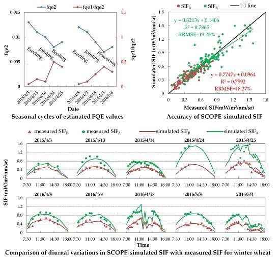
First, we evaluated the simulating accuracy of SIFB and SIFA related to both their diurnal cycles and intensities. Figure 9 displays the diurnal cycles of the half-hourly simulated SIF with fixed FQE, compared to the measured SIF on ten fieldwork days in 2015 and 2016. As illustrated, the SCOPE model can well reproduce the diurnal cycles of the SIF variation for each fieldwork day. Many studies have proven that SIF is positively correlated with PAR and GPP at the canopy scale [7,8,57,64]. Similarly, here, the simulated SIF values increase until noon and then decrease over time (with the changing of SZA), which obviously agrees with the diurnal patterns of PAR and GPP observation. Like the diurnal PAR and GPP observations shown in Figure 1 and Figure 7, the diurnal curves of SIF exhibit the same fluctuations due to unstable weather on 25 April 2015, and on 18 April and 4 May 2016. All these phenomena indicate that in the SCOPE model, the TB12 biochemical module can credibly regulate the diurnal variation of SIF emission efficiencies as a function of the dynamic micrometeorological variables. Nevertheless, on several fieldwork days—like for SIFA on 24 April 2015 or for SIFB on 3 May 2016—the systematic deviation in the diurnal SIF simulations is obvious: the simulated SIFB or SIFA values during the entire day collectively deviated from their measured points.
Table 4 concludes the quantitative assessment of the errors and deviations in SIFB and SIFA simulations with fixed FQE. This table lists the RRMSE of diurnal simulations for each fieldwork day (hereafter denoted as the daily RRMSE) and the RRMSE for all ten days of SIFA and SIFB simulations, as well as the and (as described in Section 2.4). The results show that the SCOPE model can provide acceptable accuracy for the SIFB and SIFA simulations with fixed FQE: the RRMSE values of SIFB and SIFA simulations for all 106 spectral measurements were 24.35% and 23.67%, respectively; and the daily RRMSEs were lower than 30% for each fieldwork day, except for the SIFB on 3 & 4 May 2016. Nevertheless, the systematic deviations of diurnal SIFA and SIFB simulations were noteworthy on many fieldwork days, in particular for SIFB in 3 April 2015 and 3 & 4 May 2016, and for SIFA on 24 April 2015 the absolute bias values were greater than 20%. On these days, the error in diurnal SIF simulation was mainly caused by the systematic deviation, not the inconsistency of SIF change cycles. Note that the bias variation in SIFB simulations shows a clear seasonal pattern that is coincident between 2015 and 2016. Specifically, at the erecting period (i.e., 3 April 2015 and 8 & 9 April 2016), the SIFB was underestimated with the negative bias value; but at the booting or flowering period (i.e., 24 & 25 April 2015 and 3 & 4 May 2016), the SIFB was largely overestimated with a positive bias value. These results indicated that the fixed FQE was not suitable for unbiased SIFB and SIFA simulations at all growth stages, and the unsuitable FQE values may be the major factor that caused the systematic deviations in simulated SIF. In addition, the bias values for SIFB and SIFA were mostly at different levels or even opposite in sign. For example, on 24 & 25 April 2015, the SIFA was largely underestimated, while the SIFB was overestimated; on 3 May 2016, the SIFB was greatly overestimated while the simulated SIFA values were just right. It implied that the SCOPE-simulated SIFA/SIFB with fixed FQE was probably unreliable, which should be investigated further.
Second, we evaluated the simulating accuracy of SIFA/SIFB to investigate whether the SCOPE model can reproduce the SIF spectral shape with fixed FQE. Figure 10 displays the correlation and RRMSE values between the diurnally simulated and measured SIFA/SIFB with fixed FQE for all 106 spectral measurements (Figure 10a) and the corresponding daily RRMSE for each single fieldwork day (Figure 10b). As illustrated, the SCOPE-simulated SIFA/SIFB values were not satisfying: for all 106 spectral measurements, most scatters were located far away from the 1:1 line with an R2 of only 0.0286 and an RRMSE of nearly 30%, and most daily RRMSEs were larger than 25% (with a range from 23.57% to 33.29%) on ten fieldwork days. In addition, the measured SIFA/SIFB values changed with a range from 0.593 to 3.460, while the simulated SIFA/SIFB values were relatively stable with a range from 1.552 to 2.021 across wheat’s growing season in 2015 and 2016.
Table 5 concludes the quantitative assessment of systematic deviation in the SIFA/SIFB simulations at all growth stages. The ratio of daily SIFA and SIFB averages () was calculated to express the systematic deviation, because the diurnal variations of SIFA/SIFB are dominated by the geometry of incidence and observation, making it more difficult to reflect seasonal variations of systematic deviation. As reported in Table 5, the simulated values were different from the measured ones at wheat’s erecting and booting or flowering period, with RE’s absolute value larger than 20%. Note that the RE variation in SIFA/SIFB simulations shows a consistent seasonal pattern between 2015 and 2016 that opposes the bias variation in SIFB simulations (as mentioned previously). Specifically, at the erecting period, the SIFA/SIFB values were largely overestimated with positive RE values, but at the booting or flowering period, the SIFA/SIFB values were largely underestimated with negative RE values. In addition, with fixed FQE, the SCOPE model cannot credibly reproduce the seasonal cycles of SIFA/SIFB. As the wheat grows, the measured increased from the erecting to the flowering period with a wide range from 1.370 to 2.470, while the simulated remained in the range from 1.690 to 1.916, without clear seasonal changes. These results indicated that the fixed FQE was not suitable for unbiased SIFA/SIFB simulations at all growth stages. Considering that the fqe1/fqe2 value was directly proportional to the simulated SIFA/SIFB, the unregulated fqe1/fqe2 may be the major factor limiting the seasonal variation of simulated SIFA/SIFB.
3.3.2. Variable FQE Estimated from SIF Observations
Table 6 lists the variable FQE values estimated by minimizing the systematic deviations in SIFA and SIFB simulations for each fieldwork day. For further illustration, Figure 11 displays the seasonal cycle of fqe2 and fqe1/fqe2 from the erecting to wheat’s flowering period in 2015 and 2016. As illustrated, from wheat’s erecting to its flowering stage, the fqe2 value gradually decreased from 0.013 to 0.007, while the fqe1/fqe2 value exhibited an opposite trend and increased from 0.05 to 0.5. The seasonal cycles of fqe2 and fqe1/fqe2 were consistent with variations of the systematic deviation in the SIFB and SIFA/SIFB simulations (as mentioned previously), respectively. Specifically, the fqe2 value was close to its literature-fixed value of 0.01 only at the jointing period, while at the erecting period the value was larger (0.011–0.013), and at the booting or flowering period the value was lower (0.007–0.009). Also, the fqe1/fqe2 value was close to its literature-fixed value of 0.2 only at the jointing period, while at the erecting period the value was lower (0.05–0.1), and at the booting or flowering period the value was larger (0.3–0.5). These results confirm the seasonal FQE values, showing that the seasonal cycles of FQE values between 2015 and 2016 were greatly consistent.
3.3.3. Evaluation of SIF Simulations with Variable FQE
With the above variable FQE as inputs, the systematic deviations in SIFB, SIFA, and SIFA/SIFB simulations can be corrected; meanwhile, the limited range from SIFA/SIFB simulations can be extended due to the seasonal variations of fqe1/fqe2. Thus, the SCOPE model can provide more accurate SIF simulations related to both the individual bands (SIFA and SIFB) and the seasonal SIFA/SIFB values.
On the one hand, if simulated with variable FQE values, the simulation accuracy of SIFB and SIFA can be improved greatly. Like the quantitative assessments listed in Table 4, Figure 12 displays the correlation and RRMSE values between the simulated and measured SIF with variable FQE for all 106 spectral measurements (Figure 12a) and the corresponding daily RRMSEs for each single fieldwork day (Figure 12b). As illustrated, both the simulated SIFB and SIFA were consistent with the measured ones for all 106 spectral measurements: the scatters were located close to the 1:1 line, with the R2 larger than 0.78 and an RRMSE of less than 20%. Additionally, the daily RRMSE values of SIFB and SIFA were lower than 30% (with a range from 5.97% to 29.80%) and 23% (with a range from 6.99% to 22.55%), respectively, during ten experiments in 2015 and 2016.
On the other hand, if simulated with variable FQE values, the SCOPE model can credibly reproduce the seasonal SIFA/SIFB values. Similar to Figure 12, Figure 13 shows the correlation and RRMSE values between the diurnally simulated and measured SIFA/SIFB with variable FQE. Unlike the unsatisfactory results shown in Figure 10, with variable FQE, both the range and values of simulated SIFA/SIFB were consistent with the measured ones: for all 106 spectral measurements, most scatters are close to the 1:1 line with an R2 of 0.48 and an RRMSE of only 20.63%, and most daily RRMSE were lower than 20% (with a range from 4.98% to 24.20%) on the ten fieldwork days. All these results indicated that the variable FQE settings were more suitable than the fixed ones for acquiring unbiased SIF simulations.
4. Discussion
In this study, SCOPE’s driving input parameters were derived from ten field measurements in two ways: (i) direct measurements of vegetation and meteorological parameters and (ii) a model inversion approach to retrieve LIDFa and Vcmo from in situ reflectance and GPP observations. These accurate input parameters are vital for persuasive evaluation results of the SCOPE model. The determination of these parameters is one way to calibrate the main modules related to SIF simulation. In the SCOPE model, canopy SIF emissions are propagated using three modules: the Fluspect and biochemical modules at the leaf level and the RTMo module for canopy radiative transfer of SIF signal. Vegetation parameters (e.g., LIDFa, Cab, and LAI) determine the leaf and canopy characteristics represented with the RTMo module, and the meteorological and leaf biochemical parameters (e.g., Vcmo, Rin, and Ta) determine the plant physiological and photosynthesis state represented with the biochemical module. The simulated canopy reflectance and GPP outputs separately contain information on these two aspects. So, the accuracy of reflectance and GPP simulations can reflect the joint accuracy of input parameters, which has been verified in this study.
The Vcmo values across the growing season were inverted by fitting the SCOPE model to measured GPP data. The Vcmo is one of the key parameters in the biochemical module of SCOPE for GPP modeling [20,43]. However, Poolman et al. [65,66] pointed out that the Rubisco may not be the rate limiting factor of the rate of CO2 assimilation, which means there may be some uncertainties of our method for the Vcmo estimation and new models reflecting this fact should be considered. Nevertheless, the retrieved Vcmo values match well with the literature values and show credible seasonal patterns. First, the retrieved Vcmo varied from 45 to 110 μmol m−2 s−1, which was in good accord with those displayed in the literatures for C3 crops: Vcmo ranges from 35 to 83 μmol m−2 s−1 for wheat in [61], Vcmo ranges from 76 to 136 μmol m−2 s−1 for soybean in [67], and the common Vcmo value is 93 μmol m−2 s−1 for wheat in [68,69]. Second, the retrieved Vcmo values showed plausible seasonal change patterns, which agrees well with the seasonal changes of Vcmo retrieved from space-based SIF data in [23]. To date, the possibility of prescribing Vcmo from another information source is limited. Vcmo could be estimated using leaf nitrogen content [49,70], but this estimation relied only on few experimental results, and the validation is still needed. Zhang et al. [23] retrieved the Vcmo from changes in SIF, as observed by the GOME-2 satellite, but the satellite data were aggregated over space and time with the entire growth seasons containing drought and senescence, which is different from our focus on several diurnal cycles at the canopy scale. Therefore, our model-based inversion approach for Vcmo may provide an alternative way for the estimation of Vcmo on ground or global scales. As we focus on the evaluation the SCOPE model for SIF simulation in this study, further attempts on the more accurate estimation of Vcmo was not included.
However, there are some uncertainties within the process to derive FQE. Firstly, the SIF retrieved from the spectral data was regarded as the true value for accessing the accuracy of SIF simulation. Based on this assumption, SIF simulations could be validated. However, the SIF retrieval based on 3FLD method has some uncertainties: the accuracy is dependent on the spectral characteristics of the reflectance and irradiance spectra at the absorption band, and on the spectral resolution and SNR of the sensor used. Thus, the RRMSE of simulated SIF to measured SIF is not the real error of the SCOPE model’s SIF simulation. Fortunately, the SIF observations derived from our experiments were sufficiently reliable thanks to the robust retrieval method with high spectral resolution and the SNR of the QE Pro spectrometer. According to the accuracy assessment using simulated data with the same SNR and SR of QE Pro spectrometer in [56,57], the RRMSE for the SIF retrieved using 3FLD methods is 13.2% at the O2-B band and 9.5% at the O2-A bands. Thus, the 3FLD method can retrieve SIF with sufficient accuracy and provide the reference value for evaluating SIF simulations. Therefore, the quantitative accuracy assessments made in this study can reflect the SCOPE model’s reliability.
Secondly, the vegetation parameters and meteorological or flux variables derived from in situ observations were considered accurate in this study. They also suffer from some uncertainties due to instrumental or artificial errors in field measurements. These uncertainties affect the LIDFa and Vcmo retrieval accuracy and cause an additional error in SIF simulations. According to the error propagation presented in [28], the effects of Cdm and LIDFa or Cab and LIDFa on reflectance are opposite, implying that an overestimate (underestimate) in measured Cdm or Cab will lead to an overestimate (underestimate) in the LIDFa retrievals. Moreover, the effects of Cdm and LIDFa or Cab and LIDFa on fluorescence are also opposite. Thus, the effects of a simultaneous overestimate or underestimate can to some degree cancel out in the SIF simulation. Similarly, the effect of an overestimation or underestimate of the measured LAI can also be weakened in simulated SIF, because the effects of LAI and LIDFa on reflectance and fluorescence are both accordant. Therefore, the model calibration approach of reproducing the measured reflectance spectra can to some degree weaken the impacts of vegetation parametric uncertainties on SIF simulations.
These two sources of uncertainties will propagate to our FQE estimations and then affect their variation patterns. Nevertheless, the ranges and variation patterns of our FQE values were quite consistent between two growth seasons in 2015 and 2016. Moreover, the estimated fqe2 values were close to their literature values derived from some laboratory measurements. As reported in Van der Tol et al. [25,28], the fqe2 values was around 0.01 based on the laboratory measurements in Genty et al. [33]. Trissl et al. [37] considered three different levels of fqe2 values (0.01, 0.018, and 0.021) for the modeling of PSII photochemistry. Our estimated fqe2 values seem a little lower than the fqe2 values reported in literatures (around 0.02) [35,36]. This discrepancy may be caused by the uncertainties of parameter determinations in this study, or be caused by the errors of laboratory measurements in following two aspects. First, the measured PSII fluorescence signal inevitably included the contamination of PSI fluorescence, which would cause overestimation in fqe2 [35,37,39], while our estimated fqe2 values can avoid this error, as the simulated SIF for PSII and PSI was evaluated separately. Second, the measuring flashes used for the determination of the F0-level fluorescence would cause some PSII closure, and thus the real F0-level fluorescence would be overestimated to different degrees [36]. Besides, it has been reported in several literatures that the F0-level fluorescence quantum efficiency obviously changes with different vegetation species, chlorophyll contents, and exposure of leave surfaces to the sun. Björkman and Barbara [38] measured the chlorophyll fluorescence characteristic at 77 K in 44 species of vascular plant, and found that the F0-level fluorescence signal between two different C3 species can be 2-fold variation. The variation of F0-level fluorescence signal between the lower and upper leaf surfaces or the shaded and sun leaves were also remarkable. Björkman and Barbara [38] and Morales et al. [71] also observed declines in F0-level fluorescence signal with increased chlorophyll content, probably due to an increase in the proportion of fluorescence that is reabsorbed. Moreover, as shown in Hussain et al. [72], the cinnamic acid stress will significantly reduce the efficiency of “open” PSII reaction centers in the dark-adapted state, and a tendency of increase in F0-level fluorescence was observed during 2th and 4th days. These laboratory measurements can to some degree support and account for the variation of our FQE estimations with the growth of wheat. However, the influence of different factors on FQE variations is complicated and remains unsettled. Our results can provide a reference for the parameterization of FQE values with the winter wheat in the field. More control experiments with models and in the field need to be conducted for a better understanding of the variation of FQE values.
Further opportunities are available to investigate the simulated results of MD12 and SCOPE version 1.7 compared with this study’s results. In this work, the TB12 biochemical module is generated in the SCOPE model to implement the simulations. For this module, SIF emission efficiency depends on the empirical calibration of a number of datasets collected in field and laboratory experiments. The MD12 module has a more explicit parameterization of fluorescence quenching mechanisms, while it needs two additional inputs (KNPQs and qLs) to express the intermediate conditions, which cannot be derived from our in situ measurements. Given the uncertainty in PSII-PSI fluorescence emission curves and corresponding fqe1 and fqe2 values, the PSI-PSII separation is explicitly avoided in the last version 1.7 of the SCOPE model. In the future, the SIF simulated results of this version can be evaluated and compared with this study’s results.
More field observations and theoretical simulations are required to verify the results presented in this paper. At present, we conducted the experiments only on winter wheat, and the data sets are limited. Whether the seasonal patterns of FQE variation can be applied to other species has not been ascertained. In the future, the spectral measurements should be conducted across various species and plant functional types (PFT), with more frequent time series, at different locations, in multi-angle mode, along with the observations of vegetation parameters and flux exchanges. This research could become a reality with the achievement of our automatic fluorescence observation network. Moreover, active fqe1 and fqe2 measurements with PAM should be conducted in the field and on vegetation at different growth stages, which can further verify the seasonal cycles of our variable FQE values.
5. Conclusions
In this paper, we evaluated the SCOPE model’s performance for SIFA, SIFB, and SIFA/SIFB simulations using high-accuracy spectral and flux observations in ten diurnal experiments on winter wheat. The SIF simulation accuracy with both fixed and variable FQE values was quantitatively assessed by comparison with the SIF retrieved from measurements using the 3FLD method with a QE pro spectrometer.
If simulated with fixed FQE values, the SCOPE model can reliably interpret SIF diurnal cycles and provide acceptable results for SIFB and SIFA simulations. The RRMSEs of SIFA and SIFB for all 106 spectral measurements in the ten diurnal experiments were 24.35% and 23.67%, respectively. Nevertheless, the fixed FQE values were not suitable for wheat at all growth stages. At wheat’s erecting period and at its booting or flowering period, the systematical deviations in SIFB and SIFA/SIFB simulations were noteworthy, and the seasonal cycles of SIFA/SIFB cannot be credibly reproduced, with a low determination coefficient (R2) of 0.0286.
When the SIF simulation was conducted with variable FQE values, which vary with the growth of wheat, its accuracy was improved greatly. Specifically, the SCOPE model can accurately simulate the SIFB and SIFA with RRMSEs of 18.27% and 19.25%, respectively, and the SCOPE simulations track well with the seasonal SIFA/SIFB values with an RRMSE of 20.63% and a determination coefficient (R2) of 0.48. The results indicated a clear seasonal pattern of suitable FQE values. When the growth stage changed from the erecting to the flowering stage, the fqe1/fqe2 increased from approximately 0.05–0.1 to approximately 0.3–0.5, while the fqe2 decreased from 0.013 to 0.07.
Therefore, although the SCOPE model can credibly simulate canopy SIF, the input FQE values should be carefully determined. Seasonal changes of the FQE values or the FQE values’ dependence on plant physiological status cannot be ignored for accurate simulations of canopy SIF. Our quantitative results of the model assessment and FQE adjustment can serve as a significant reference for future application of the SCOPE model. However, the study is preliminary; more experiments are needed to determine FQE values in the SCOPE model.
Acknowledgments
This research was supported by the National Key Research and Development Program of China (2017YFA0603001), and the National Natural Science Foundation of China (41701396). The authors are thankful to Christiaan Van der Tol for providing the SCOPE model. We thank the anonymous reviewers for providing comments that helped to improve the quality of the original manuscript.
Author Contributions
Jiaochan Hu was primarily responsible for mathematical modeling and experimental design. Xinjie Liu improved the experimental analysis and revised the paper. Liangyun Liu contributed to the original idea for the research and to the experimental design. Linlin Guan provided support regarding the application of Diurnal flux and meteorological observations.
Conflicts of Interest
The authors declare no conflict of interest.
References
- Pedrós, R.; Moya, I.; Goulas, Y.; Jacquemoud, S. Chlorophyll fluorescence emission spectrum inside a leaf. Photochem. Photobiol. Sci. 2008, 7, 498–502. [Google Scholar] [CrossRef] [PubMed]
- Zarco-Tejada, P.J. Hyperspectral Remote Sensing of Closed Forest Canopies: Estimation of Chlorophyll Fluorescence and Pigment Content. Ph.D. Thesis, York University Toronto, Toronto, ON, Canada, December 2000. [Google Scholar]
- Pfündel, E. Estimating the contribution of photosystem i to total leaf chlorophyll fluorescence. Photosynth. Res. 1998, 56, 185–195. [Google Scholar] [CrossRef]
- Krause, G.H.; Weis, E. Chlorophyll fluorescence and photosynthesis—The basics. Ann. Rev. Plant Biol. 1991, 42, 313–349. [Google Scholar] [CrossRef]
- Porcar-Castell, A.; Tyystjärvi, E.; Atherton, J.; van der Tol, C.; Flexas, J.; Pfündel, E.E.; Moreno, J.; Frankenberg, C.; Berry, J.A. Linking chlorophyll a fluorescence to photosynthesis for remote sensing applications: Mechanisms and challenges. J. Exp. Bot. 2014, 65, 4065–4095. [Google Scholar] [CrossRef] [PubMed]
- Lichtenthaler, H.K.; Rinderle, U. The role of chlorophyll fluorescence in the detection of stress conditions in plants. CRC Crit. Rev. Anal. Chem. 1988, 19, S29–S85. [Google Scholar] [CrossRef]
- Damm, A.; Elbers, J.A.N.; Erler, A.; Gioli, B.; Hamdi, K.; Hutjes, R.; Kosvancova, M.; Meroni, M.; Miglietta, F.; Moersch, A.; et al. Remote sensing of sun-induced fluorescence to improve modeling of diurnal courses of gross primary production (GPP). Glob. Chang. Biol. 2010, 16, 171–186. [Google Scholar] [CrossRef] [Green Version]
- Damm, A.; Guanter, L.; Paul-Limoges, E.; van der Tol, C.; Hueni, A.; Buchmann, N.; Eugster, W.; Ammann, C.; Schaepman, M.E. Far-red sun-induced chlorophyll fluorescence shows ecosystem-specific relationships to gross primary production: An assessment based on observational and modeling approaches. Remote Sens. Environ. 2015, 166, 91–105. [Google Scholar] [CrossRef]
- Guanter, L.; Zhang, Y.; Jung, M.; Joiner, J.; Voigt, M.; Berry, J.A.; Frankenberg, C.; Huete, A.R.; Zarco-Tejada, P.; Lee, J.-E. Global and time-resolved monitoring of crop photosynthesis with chlorophyll fluorescence. Proc. Natl. Acad. Sci. USA 2014, 111, 1327–1333. [Google Scholar] [CrossRef] [PubMed]
- Liu, L.; Guan, L.; Liu, X. Directly estimating diurnal changes in GPP for C3 and C4 crops using far-red sun-induced chlorophyll fluorescence. Agric. For. Meteorol. 2017, 232, 1–9. [Google Scholar] [CrossRef]
- Yang, X.; Tang, J.; Mustard, J.F.; Lee, J.E.; Rossini, M.; Joiner, J.; Munger, J.W.; Kornfeld, A.; Richardson, A.D. Solar-induced chlorophyll fluorescence that correlates with canopy photosynthesis on diurnal and seasonal scales in a temperate deciduous forest. Geophys. Res. Lett. 2015, 42, 2977–2987. [Google Scholar] [CrossRef]
- Plascyk, J.A. The MK II fraunhofer line discriminator (FLD-II) for airborne and orbital remote sensing of solar-stimulated luminescence. Opt. Eng. 1975, 14, 339–346. [Google Scholar] [CrossRef]
- Meroni, M.; Rossini, M.; Guanter, L.; Alonso, L.; Rascher, U.; Colombo, R.; Moreno, J. Remote sensing of solar-induced chlorophyll fluorescence: Review of methods and applications. Remote Sens. Environ. 2009, 113, 2037–2051. [Google Scholar] [CrossRef]
- Frankenberg, C.; Fisher, J.B.; Worden, J.; Badgley, G.; Saatchi, S.S.; Lee, J.E.; Toon, G.C.; Butz, A.; Jung, M.; Kuze, A.; et al. New global observations of the terrestrial carbon cycle from GOSAT: Patterns of plant fluorescence with gross primary productivity. Geophys. Res. Lett. 2011, 38, 351–365. [Google Scholar] [CrossRef]
- Frankenberg, C.; O’Dell, C.; Berry, J.; Guanter, L.; Joiner, J.; Köhler, P.; Pollock, R.; Taylor, T.E. Prospects for chlorophyll fluorescence remote sensing from the orbiting carbon observatory-2. Remote Sens. Environ. 2014, 147, 1–12. [Google Scholar] [CrossRef]
- Guanter, L.; Frankenberg, C.; Dudhia, A.; Lewis, P.E.; Gómez-Dans, J.; Kuze, A.; Suto, H.; Grainger, R.G. Retrieval and global assessment of terrestrial chlorophyll fluorescence from gosat space measurements. Remote Sens. Environ. 2012, 121, 236–251. [Google Scholar] [CrossRef]
- Joiner, J.; Yoshida, Y.; Vasilkov, A.P.; Corp, L.A.; Middleton, E.M. First observations of global and seasonal terrestrial chlorophyll fluorescence from space. Biogeosciences 2011, 8, 637–651. [Google Scholar] [CrossRef] [Green Version]
- Joiner, J.; Guanter, L.; Lindstrot, R.; Voigt, M.; Vasilkov, A.P.; Middleton, E.M.; Huemmrich, K.F.; Yoshida, Y.; Frankenberg, C. Global monitoring of terrestrial chlorophyll fluorescence from moderate spectral resolution near-infrared satellite measurements: Methodology, simulations, and application to gome-2. Atmos. Meas. Tech. 2013, 6, 2803–2823. [Google Scholar] [CrossRef]
- Guan, K.; Berry, J.A.; Zhang, Y.; Joiner, J.; Guanter, L.; Badgley, G.; Lobell, D.B. Improving the monitoring of crop productivity using spaceborne solar-induced fluorescence. Glob. Chang. Biol. 2016, 22, 716–726. [Google Scholar] [CrossRef] [PubMed]
- Van der Tol, C.; Verhoef, W.; Timmermans, J.; Verhoef, A.; Su, Z. An integrated model of soil-canopy spectral radiances, photosynthesis, fluorescence, temperature and energy balance. Biogeosciences 2009, 6, 3109–3129. [Google Scholar] [CrossRef]
- Liu, X.; Liu, L. Improving chlorophyll fluorescence retrieval using reflectance reconstruction based on principal components analysis. IEEE Geosci. Remote Sens. Lett. 2015, 12, 1645–1649. [Google Scholar]
- Liu, X.; Liu, L.; Zhang, S.; Zhou, X. New spectral fitting method for full-spectrum solar-induced chlorophyll fluorescence retrieval based on principal components analysis. Remote Sens. 2015, 7, 10626–10645. [Google Scholar] [CrossRef]
- Zhang, Y.; Guanter, L.; Berry, J.A.; Joiner, J.; van der Tol, C.; Huete, A.; Gitelson, A.; Voigt, M.; Kohler, P. Estimation of vegetation photosynthetic capacity from space-based measurements of chlorophyll fluorescence for terrestrial biosphere models. Glob. Chang. Biol. 2014, 20, 3727–3742. [Google Scholar] [CrossRef] [PubMed]
- Verrelst, J.; van der Tol, C.; Magnani, F.; Sabater, N.; Rivera, J.P.; Mohammed, G.; Moreno, J. Evaluating the predictive power of sun-induced chlorophyll fluorescence to estimate net photosynthesis of vegetation canopies: A scope modeling study. Remote Sens. Environ. 2016, 176, 139–151. [Google Scholar] [CrossRef]
- Van der Tol, C.; Berry, J.; Campbell, P.; Rascher, U. Models of fluorescence and photosynthesis for interpreting measurements of solar-induced chlorophyll fluorescence. J. Geophys. Res. Biogeosci. 2014, 119, 2312–2327. [Google Scholar] [CrossRef] [PubMed] [Green Version]
- Koffi, E.; Rayner, P.; Norton, A.; Frankenberg, C.; Scholze, M. Investigating the usefulness of satellite derived fluorescence data in inferring gross primary productivity within the carbon cycle data assimilation system. Biogeosci. Discuss. 2015, 12, 707–749. [Google Scholar] [CrossRef]
- Lee, J.E.; Berry, J.A.; Tol, C.; Yang, X.; Guanter, L.; Damm, A.; Baker, I.; Frankenberg, C. Simulations of chlorophyll fluorescence incorporated into the Community Land Model version 4. Glob. Chang Biol. 2015, 21, 3469–3477. [Google Scholar] [CrossRef] [PubMed] [Green Version]
- Van der Tol, C.; Rossini, M.; Cogliati, S.; Verhoef, W.; Colombo, R.; Rascher, U.; Mohammed, G. A model and measurement comparison of diurnal cycles of sun-induced chlorophyll fluorescence of crops. Remote Sens. Environ. 2016, 186, 663–677. [Google Scholar] [CrossRef]
- Verrelst, J.; Rivera, J.P.; van der Tol, C.; Magnani, F.; Mohammed, G.; Moreno, J. Global sensitivity analysis of the scope model: What drives simulated canopy-leaving sun-induced fluorescence? Remote Sens. Environ. 2015, 166, 8–21. [Google Scholar] [CrossRef]
- Agati, G.; Mazzinghi, P.; Fusi, F.; Ambrosini, I. The F685/F730 chlorophyll fluorescence ratio as a tool in plant physiology: Response to physiological and environmental factors. J. Plant Physiol. 1995, 145, 228–238. [Google Scholar] [CrossRef]
- Cheng, Y.-B.; Middleton, E.; Zhang, Q.; Huemmrich, K.; Campbell, P.; Corp, L.; Cook, B.; Kustas, W.; Daughtry, C. Integrating solar induced fluorescence and the photochemical reflectance index for estimating gross primary production in a cornfield. Remote Sens. 2013, 5, 6857–6879. [Google Scholar] [CrossRef]
- Gitelson, A.A.; Buschmann, C.; Lichtenthaler, H.K. Leaf chlorophyll fluorescence corrected for re-absorption by means of absorption and reflectance measurements. J. Plant Physiol. 1998, 152, 283–296. [Google Scholar] [CrossRef]
- Genty, B.; Briantais, J.M.; Baker, N.R. The relationship between the quantum yield of photosynthetic electron transport and quenching of chlorophyll fluorescence. BBA—Gen. Subj. 1989, 990, 87–92. [Google Scholar] [CrossRef]
- Lazár, D. Chlorophyll a fluorescence induction. Biochim. Biophys. Acta 1999, 1412, 1–28. [Google Scholar] [CrossRef]
- Lazár, D. Chlorophyll a fluorescence rise induced by high light illumination of dark-adapted plant tissue studied by means of a model of photosystem II and considering photosystem II heterogeneity. J. Theor. Biol. 2003, 220, 469–503. [Google Scholar] [CrossRef] [PubMed]
- Lazár, D. Parameters of photosynthetic energy partitioning. J. Plant Physiol. 2015, 175, 131–147. [Google Scholar] [CrossRef] [PubMed]
- Trissl, H.W.; Gao, Y.; Wulf, K. Theoretical fluorescence induction curves derived from coupled differential equations describing the primary photochemistry of photosystem II by an exciton-radical pair equilibrium. Biophys. J. 1993, 64, 974–988. [Google Scholar] [CrossRef]
- Björkman, O.; Barbara, D. Photon yield of O2 evolution and chlorophyll fluorescence characteristics at 77 K among vascular plants of diverse origins. Planta 1987, 170, 489–504. [Google Scholar] [CrossRef] [PubMed]
- Lazár, D. Simulations show that a small part of variable chlorophyll a, fluorescence originates in photosystem I and contributes to overall fluorescence rise. J. Theor. Biol. 2013, 335, 249–264. [Google Scholar] [CrossRef] [PubMed]
- Weis, E.; Berry, J.A. Quantum efficiency of photosystem II in relation to energy-dependent quenching of chlorophyll fluorescence. Biochim. Biophys. Acta (BBA)-Bioenerg. 1987, 894, 198–208. [Google Scholar] [CrossRef]
- Verhoef, W. Light scattering by leaf layers with application to canopy reflectance modeling: The SAIL model. Remote Sens. Environ. 1984, 16, 125–141. [Google Scholar] [CrossRef]
- Jacquemoud, S.; Baret, F. PROSPECT: A model of leaf optical properties spectra. Remote Sens. Environ. 1990, 34, 75–91. [Google Scholar] [CrossRef]
- Farquhar, G.D.; von Caemmerer, S.; Berry, J.A. A biochemical model of photosynthetic CO2 assimilation in leaves of C3 species. Planta 1980, 149, 78–90. [Google Scholar] [CrossRef] [PubMed]
- Von Caemmerer, S. Steady-state models of photosynthesis. Plant Cell Environ. 2013, 36, 1617–1630. [Google Scholar] [CrossRef] [PubMed]
- Collatz, G.J.; Ball, J.T.; Grivet, C.; Berry, J.A. Physiological and environmental regulation of stomatal conductance, photosynthesis and transpiration: A model that includes a laminar boundary layer. Agric. For. Meteorol. 1991, 54, 107–136. [Google Scholar] [CrossRef]
- Collatz, G.J.; Ribas-Carbo, M.; Berry, J.A. Coupled photosynthesis–stomatal conductance model for leaves of C4 plants. Aust. J. Plant Physiol. 1992, 19, 519–538. [Google Scholar] [CrossRef]
- Magnani, F.; Olioso, A.; Demarty, J.; Germain, V.; Verhoef, W.; Moya, I.; Van der Tol, C. Assessment of Vegetation Photosynthesis through Observation of Solar Induced Fluorescence from Space. In Final Report for the European Space Agency under ESTEC Contract No. 20678/07/NL/HE; ESA: Paris, France, 2009. [Google Scholar]
- Porcar-Castell, A. A high-resolution portrait of the annual dynamics of photochemical and non-photochemical quenching in needles of Pinus sylvestris. Physiol. Plant. 2011, 143, 139–153. [Google Scholar] [CrossRef] [PubMed]
- Xu, L.; Baldocchi, D.D. Seasonal trends in photosynthetic parameters and stomatal conductance of blue oak (Quercus douglasii) under prolonged summer drought and high temperature. Tree Physiol. 2003, 23, 865–877. [Google Scholar] [CrossRef] [PubMed]
- Goel, N.S.; Strebel, D.E. Simple beta distribution representation of leaf orientation in vegetation canopies. Agron. J. 1984, 76, 800–802. [Google Scholar] [CrossRef]
- Liu, L.; Wang, J.; Bao, Y.; Huang, W.; Ma, Z.; Zhao, C. Predicting winter wheat condition, grain yield and protein content using multi-temporal EnviSat-ASAR and Landsat TM satellite images. Int. J. Remote Sens. 2006, 27, 737–753. [Google Scholar] [CrossRef]
- Ergun, E.; Demirata, B.; Gumus, G.; Apak, R. Simultaneous determination of chlorophyll a and chlorophyll b by derivative spectrophotometry. Anal. Bioanal. Chem. 2004, 379, 803–811. [Google Scholar] [CrossRef] [PubMed]
- Falge, E.; Baldocchi, D.; Olson, R.; Anthoni, P.; Aubinet, M.; Bernhofer, C.; Burba, G.; Ceulemans, R.; Clement, R.; Dolman, H. Gap filling strategies for defensible annual sums of net ecosystem exchange. Agric. For. Meteorol. 2001, 107, 43–69. [Google Scholar] [CrossRef]
- Reichstein, M.; Falge, E.; Baldocchi, D.; Papale, D.; Aubinet, M.; Berbigier, P.; Bernhofer, C.; Buchmann, N.; Gilmanov, T.; Granier, A. On the separation of net ecosystem exchange into assimilation and ecosystem respiration: Review and improved algorithm. Glob. Chang. Biol. 2005, 11, 1424–1439. [Google Scholar] [CrossRef]
- Plascyk, J.A.; Gabriel, F.C. Fraunhofer line discriminator MK II—Airborne instrument for precise and standardized ecological luminescence measurement. IEEE Trans. Instrum. Meas. 1975, 24, 306–313. [Google Scholar] [CrossRef]
- Liu, L.; Liu, X.; Hu, J. Effects of spectral resolution and SNR on the vegetation solar-induced fluorescence retrieval using FLD-based methods at canopy level. Eur. J. Remote Sens. 2015, 48, 743–762. [Google Scholar] [CrossRef]
- Liu, L.; Liu, X.; Hu, J.; Guan, L. Assessing the wavelength-dependent ability of solar-induced chlorophyll fluorescence to estimate the GPP of winter wheat at the canopy level. Int. J. Remote Sens. 2017, 38, 4396–4417. [Google Scholar] [CrossRef]
- Maier, S.W.; Günther, K.P.; Stellmes, M. Sun-induced fluorescence: A new tool for precision farming. In Digital Imaging and Spectral Techniques: Applications to Precision Agriculture and Crop Physiology; Kral, D.M., Barbarick, K.A., Volenec, J.J., Dick, W.A., Eds.; American Society of Agronomy Special Publication: Madison, WI, USA, 2003; pp. 209–222. [Google Scholar]
- Wullschleger, S.D. Biochemical Limitations to Carbon Assimilation in C3 Plants—A Retrospective Analysis of the A/Ci Curves from 109 Species. J. Exp. Bot. 1993, 44, 907–920. [Google Scholar] [CrossRef]
- Sellers, P.J.; Dickinson, R.E.; Randall, D.A.; Betts, A.K.; Hall, F.G.; Berry, J.A.; Collatz, G.J.; Denning, A.S.; Mooney, H.A.; Nobre, C.A.; et al. Modeling the exchanges of energy, water, and carbon between continents and the atmosphere. Science 1997, 275, 502–509. [Google Scholar] [CrossRef] [PubMed]
- Kattge, J.; Knorr, W.; Raddatz, T.; Wirth, C. Quantifying photosynthetic capacity and its relationship to leaf nitrogen content for global scale terrestrial biosphere models. Glob. Chang. Biol. 2009, 15, 976–991. [Google Scholar] [CrossRef]
- Mäkelä, A.; Hari, P.; Berninger, F.; Hänninen, H.; Nikinmaa, E. Acclimation of photosynthetic capacity in Scots pine to the annual cycle of temperature. Tree Physiol. 2004, 24, 369–376. [Google Scholar] [CrossRef] [PubMed]
- Wolf, A.; Akshalov, K.; Saliendra, N.; Johnson, D.A.; Laca, E.A. Inverse estimation of Vcmax, leaf area index, and the Ball-Berry parameter from carbon and energy fluxes. J. Geophys. Res. Atmos. 2006, 111, 1003–1019. [Google Scholar] [CrossRef]
- Liu, L.; Zhang, Y.; Wang, J.; Zhao, C. Detecting solar-induced chlorophyll fluorescence from field radiance spectra based on the fraunhofer line principle. IEEE Trans. Geosci. Remote Sens. 2005, 43, 827–832. [Google Scholar]
- Poolman, M.G.; Fell, D.A.; Thomas, S. Modelling photosynthesis and its control. J. Exp. Bot. 2000, 51, 319–328. [Google Scholar] [CrossRef] [PubMed]
- Poolman, M.G.; Olçer, H.; Lloyd, J.C.; Raines, C.A.; Fell, D.A. Computer modelling and experimental evidence for two steady states in the photosynthetic Calvin cycle. Eur. J. Biochem. 2001, 268, 2810–2816. [Google Scholar] [CrossRef] [PubMed]
- Ainsworth, E.A.; Serbin, S.P.; Skoneczka, J.A.; Townsend, P.A. Using leaf optical properties to detect ozone effects on foliar biochemistry. Photosynth. Res. 2014, 119, 65–76. [Google Scholar] [CrossRef] [PubMed]
- Kothavala, Z.; Arain, M.A.; Black, T.A.; Verseghy, D. The simulation of energy, water vapor and carbon dioxide fluxes over common crops by the Canadian Land Surface Scheme (CLASS). Agric. For. Meteorol. 2005, 133, 89–108. [Google Scholar] [CrossRef]
- Lokupitiya, E.; Denning, S.; Paustian, K.; Baker, I.; Schaefer, K.; Verma, S.B.; Meyers, T.; Bernacchi, C.J.; Suyker, A.E.; Fischer, M. Incorporation of crop phenology in Simple Biosphere model (SiBcrop) to improve land-atmosphere carbon exchanges from croplands. Biogeosciences 2009, 6, 969–986. [Google Scholar] [CrossRef]
- Wilson, K.B.; Baldocchi, D.D.; Hanson, P.J. Spatial and seasonal variability of photosynthetic parameters and their relationship to leaf nitrogen in a deciduous forest. Tree Physiol. 2000, 20, 565–578. [Google Scholar] [CrossRef] [PubMed]
- Morales, F.; Abadía, A.; Abadía, J. Chlorophyll Fluorescence and Photon Yield of Oxygen Evolution in Iron-Deficient Sugar Beet (Beta vulgaris L.) Leaves. Plant Physiol. 1991, 97, 886–893. [Google Scholar] [CrossRef] [PubMed]
- Hussain, M.I.; Reigosa, M.J. A chlorophyll fluorescence analysis of photosynthetic efficiency, quantum yield and photon energy dissipation in PSII antennae of Lactuca sativa L. leaves exposed to cinnamic acid. Plant Physiol. Biochem. 2011, 49, 1290–1298. [Google Scholar] [CrossRef] [PubMed]
Figure 1.
Diurnal observations of meteorological parameters between 7:00 to 19:00 made during ten experiments in 2015 and 2016: (a) half-hour air temperature and VPD observations and (b) half-hour PAR observations.
Figure 1.
Diurnal observations of meteorological parameters between 7:00 to 19:00 made during ten experiments in 2015 and 2016: (a) half-hour air temperature and VPD observations and (b) half-hour PAR observations.

Figure 2.
Schematic overview of the LIDFa inversion procedure.

Figure 3.
Schematic overview of the Vcmo inversion procedure.

Figure 4.
Schematic overview of SIF simulations and model evaluation.

Figure 5.
The simulated and measured reflectance spectra and their residuals at 10:00 for every fieldwork day in 2015 and 2016.
Figure 5.
The simulated and measured reflectance spectra and their residuals at 10:00 for every fieldwork day in 2015 and 2016.

Figure 6.
Root mean squared error (RMSE) values between the simulated and measured reflectance spectra for 106 spectral measurements in 2015 and 2016.
Figure 6.
Root mean squared error (RMSE) values between the simulated and measured reflectance spectra for 106 spectral measurements in 2015 and 2016.

Figure 7.
The diurnal cycles of simulated and measured GPP at half-hour intervals between 7:00 and 19:00 on ten fieldwork days in 2015 and 2016.
Figure 7.
The diurnal cycles of simulated and measured GPP at half-hour intervals between 7:00 and 19:00 on ten fieldwork days in 2015 and 2016.

Figure 8.
The correlation and relative root mean square error (RRMSE) value between simulated and measured GPP for all half-hour flux observations during ten experiments in 2015 and 2016.
Figure 8.
The correlation and relative root mean square error (RRMSE) value between simulated and measured GPP for all half-hour flux observations during ten experiments in 2015 and 2016.

Figure 9.
The diurnal cycles of simulated SIF with fixed FQE, compared to the measured SIF at O2-B and O2-A bands on ten fieldwork days in 2015 and 2016.
Figure 9.
The diurnal cycles of simulated SIF with fixed FQE, compared to the measured SIF at O2-B and O2-A bands on ten fieldwork days in 2015 and 2016.

Figure 10.
The correlation and relative root mean square error (RRMSE) values between simulated and measured SIFA/SIFB with fixed FQE: (a) the correlation and RRMSE for 106 spectral measurements and (b) the RRMSE values for each fieldwork day in 2015 and 2016.
Figure 10.
The correlation and relative root mean square error (RRMSE) values between simulated and measured SIFA/SIFB with fixed FQE: (a) the correlation and RRMSE for 106 spectral measurements and (b) the RRMSE values for each fieldwork day in 2015 and 2016.

Figure 11.
The seasonal cycles of fqe2 and fqe1/fqe2 on ten fieldwork days in 2015 and 2016.

Figure 12.
The correlation and relative root mean square error (RRMSE) values between simulated and measured SIFA and SIFB with variable FQE: (a) the correlation and RRMSE for 106 spectral measurements and (b) the RRMSE values for each fieldwork day in 2015 and 2016.
Figure 12.
The correlation and relative root mean square error (RRMSE) values between simulated and measured SIFA and SIFB with variable FQE: (a) the correlation and RRMSE for 106 spectral measurements and (b) the RRMSE values for each fieldwork day in 2015 and 2016.

Figure 13.
The correlation and relative root mean square error (RRMSE) values between simulated and measured SIFA/SIFB with variable FQE: (a) the correlation and RRMSE for 106 spectral measurements and (b) the RRMSE values for each fieldwork day in 2015 and 2016.
Figure 13.
The correlation and relative root mean square error (RRMSE) values between simulated and measured SIFA/SIFB with variable FQE: (a) the correlation and RRMSE for 106 spectral measurements and (b) the RRMSE values for each fieldwork day in 2015 and 2016.


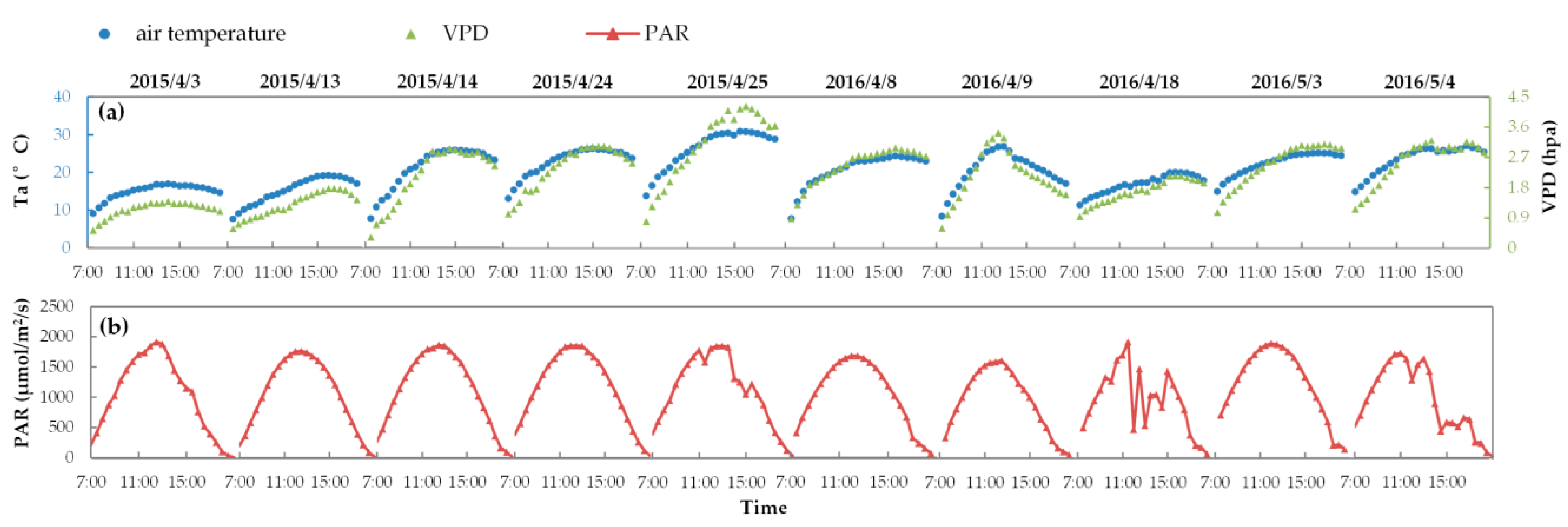
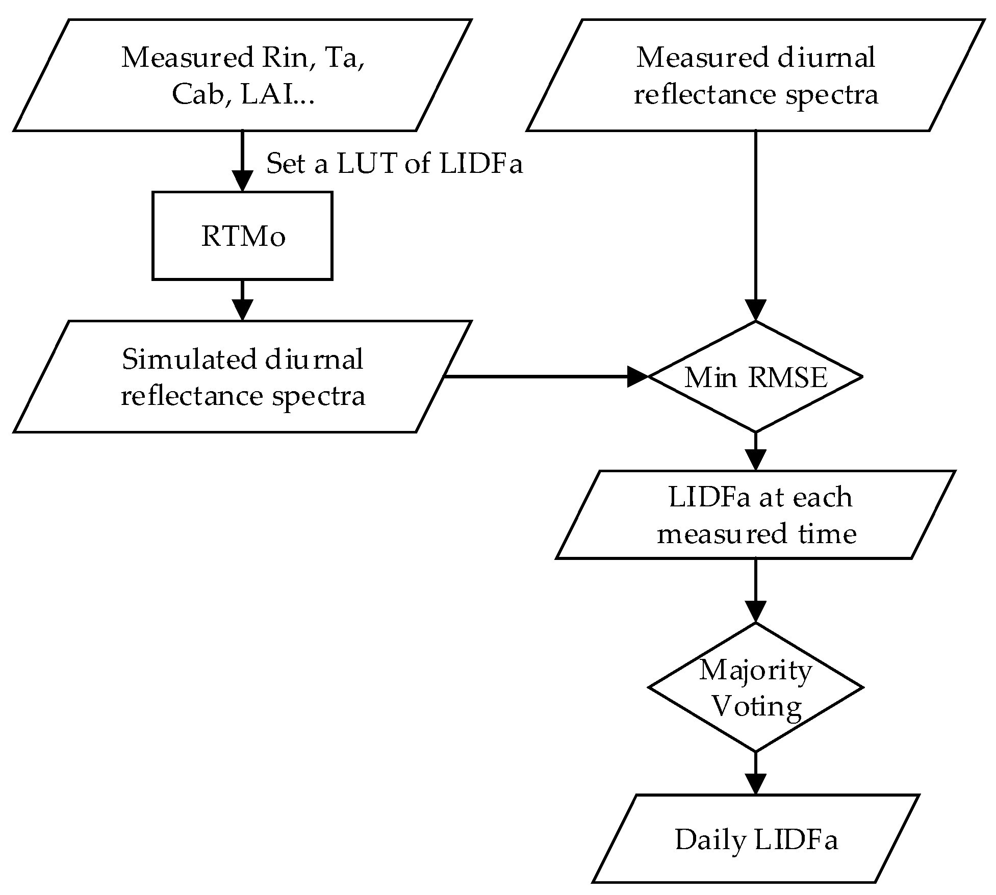
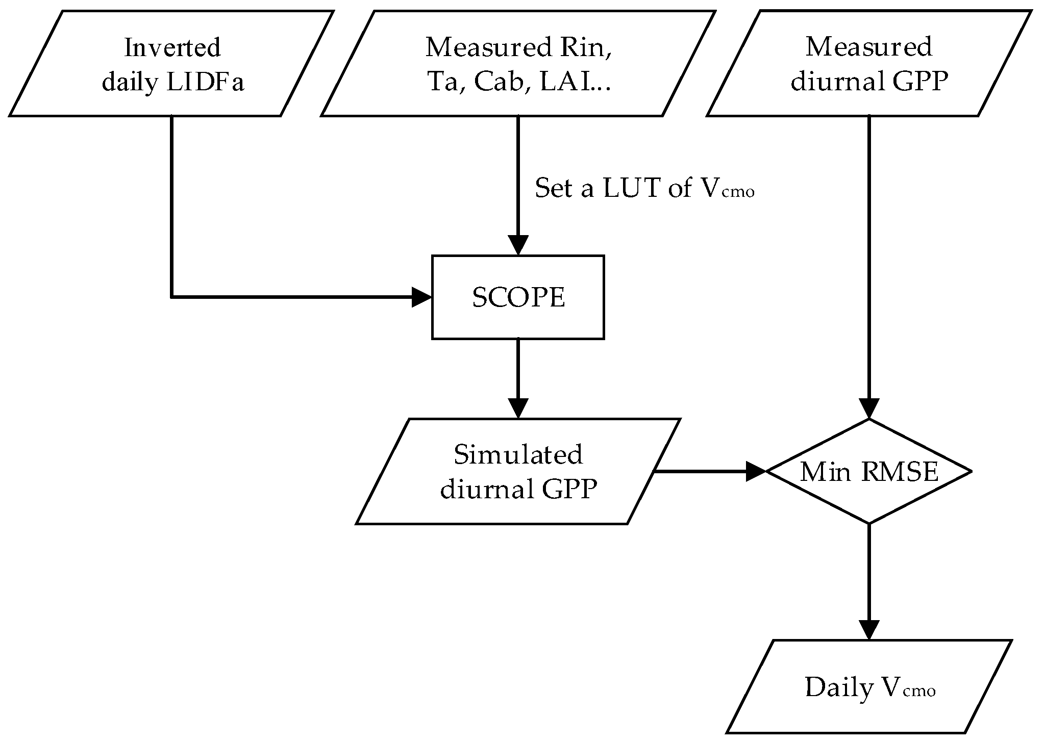
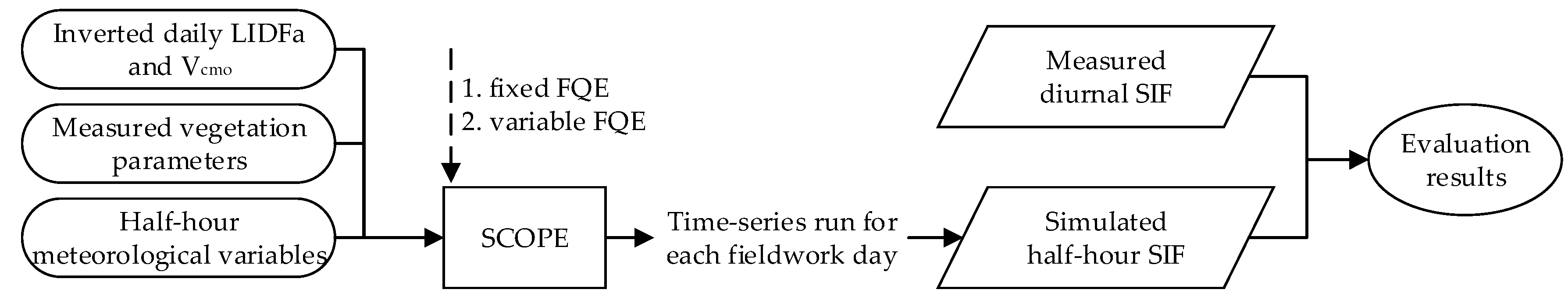
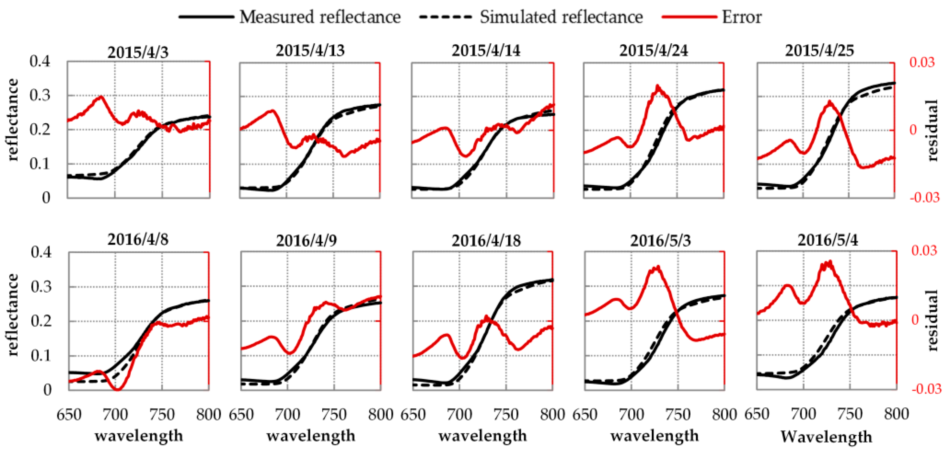
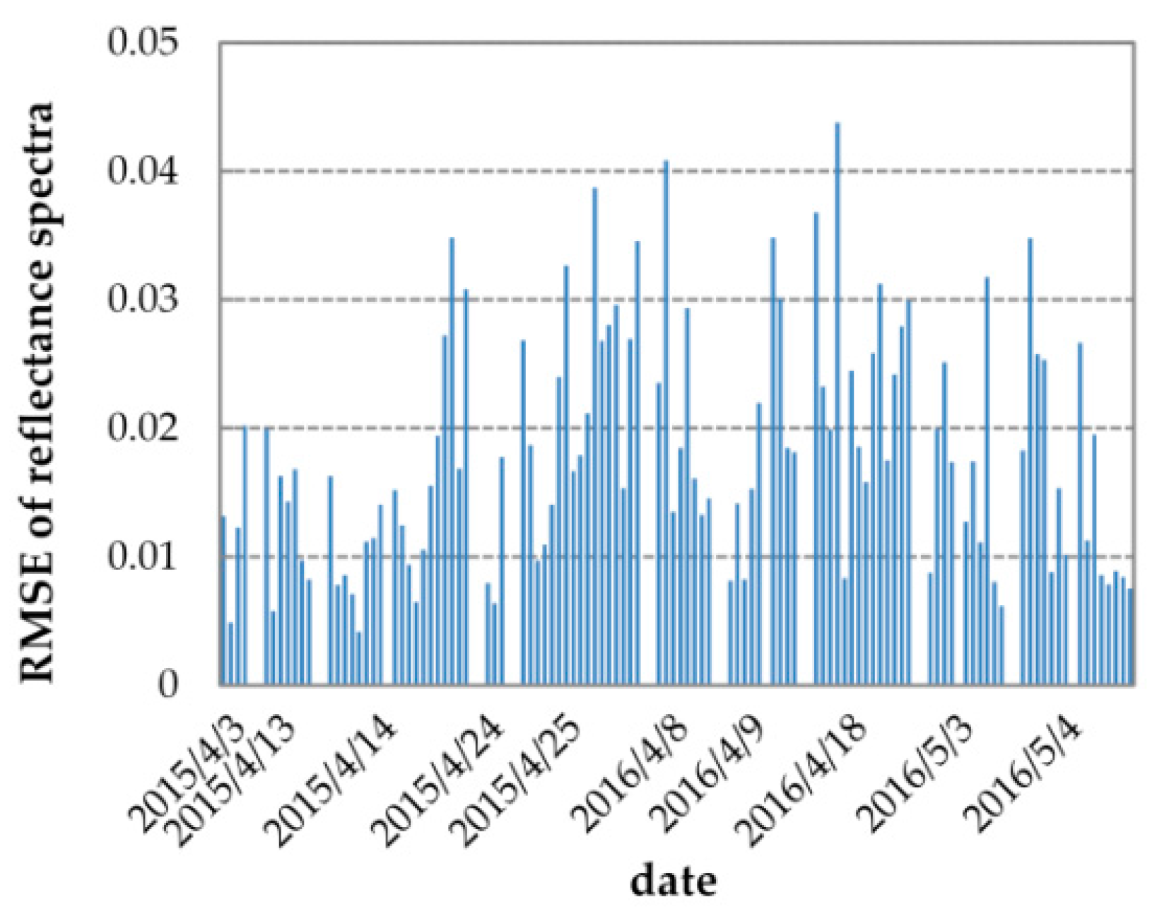
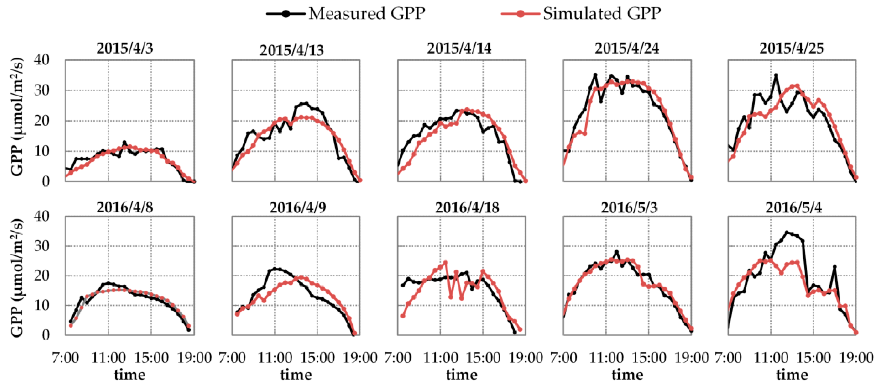
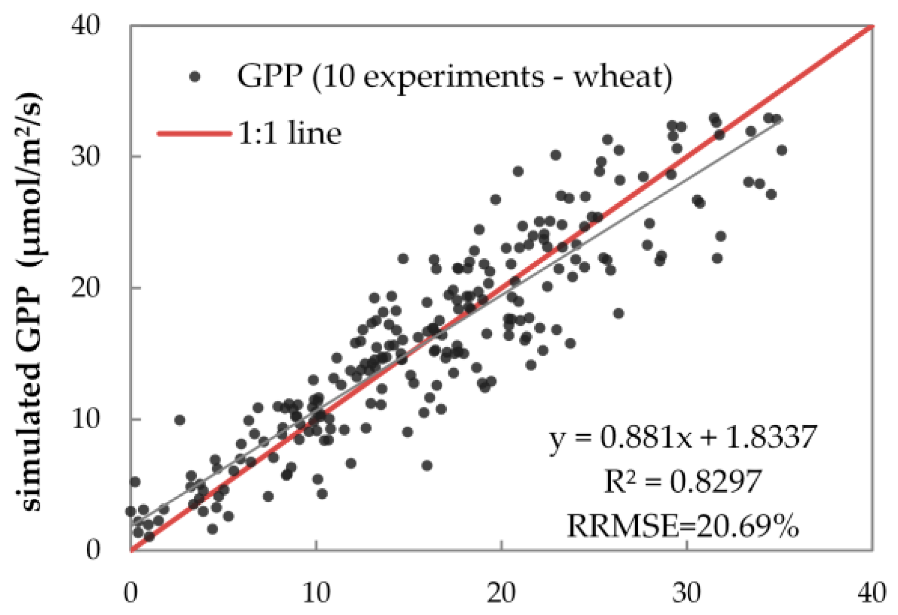
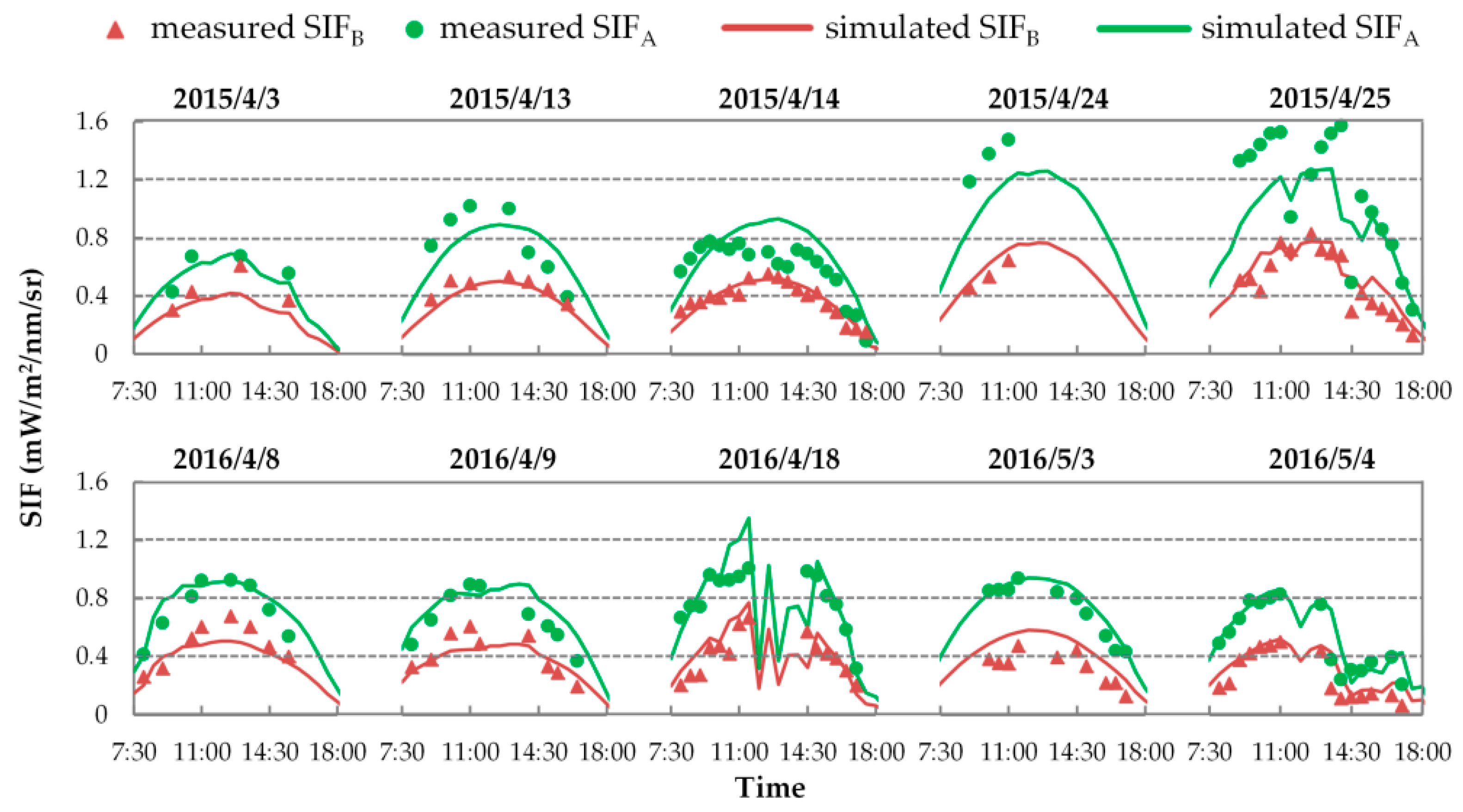
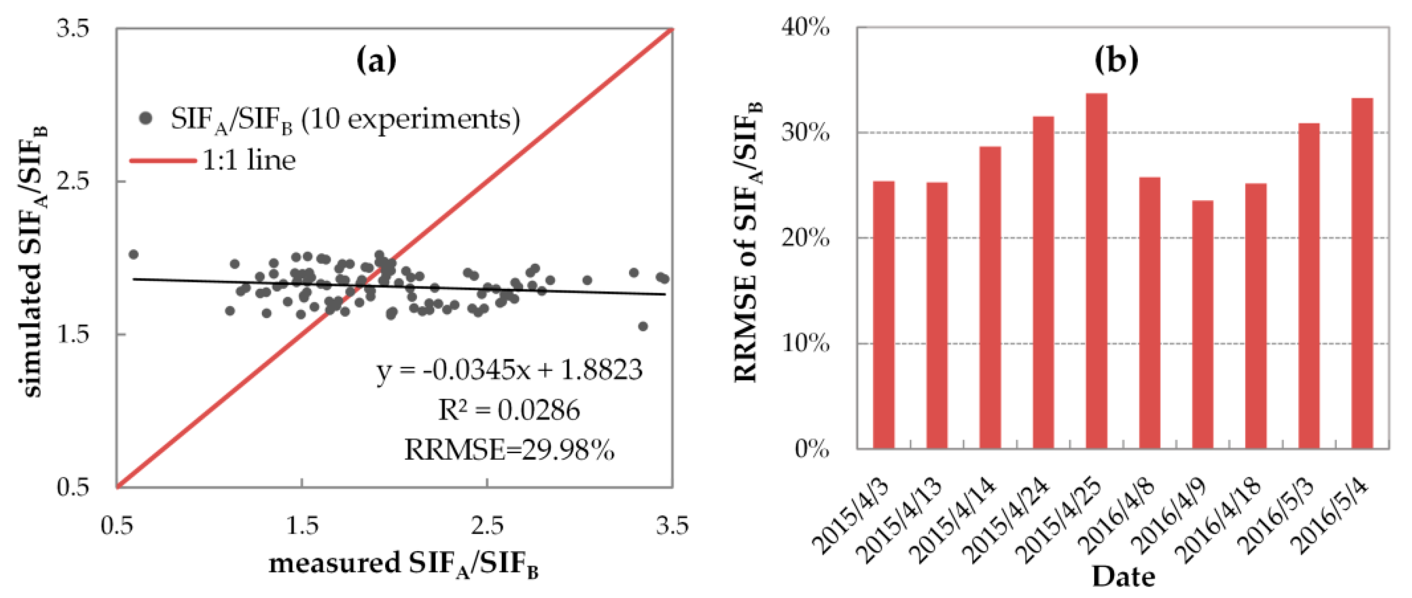
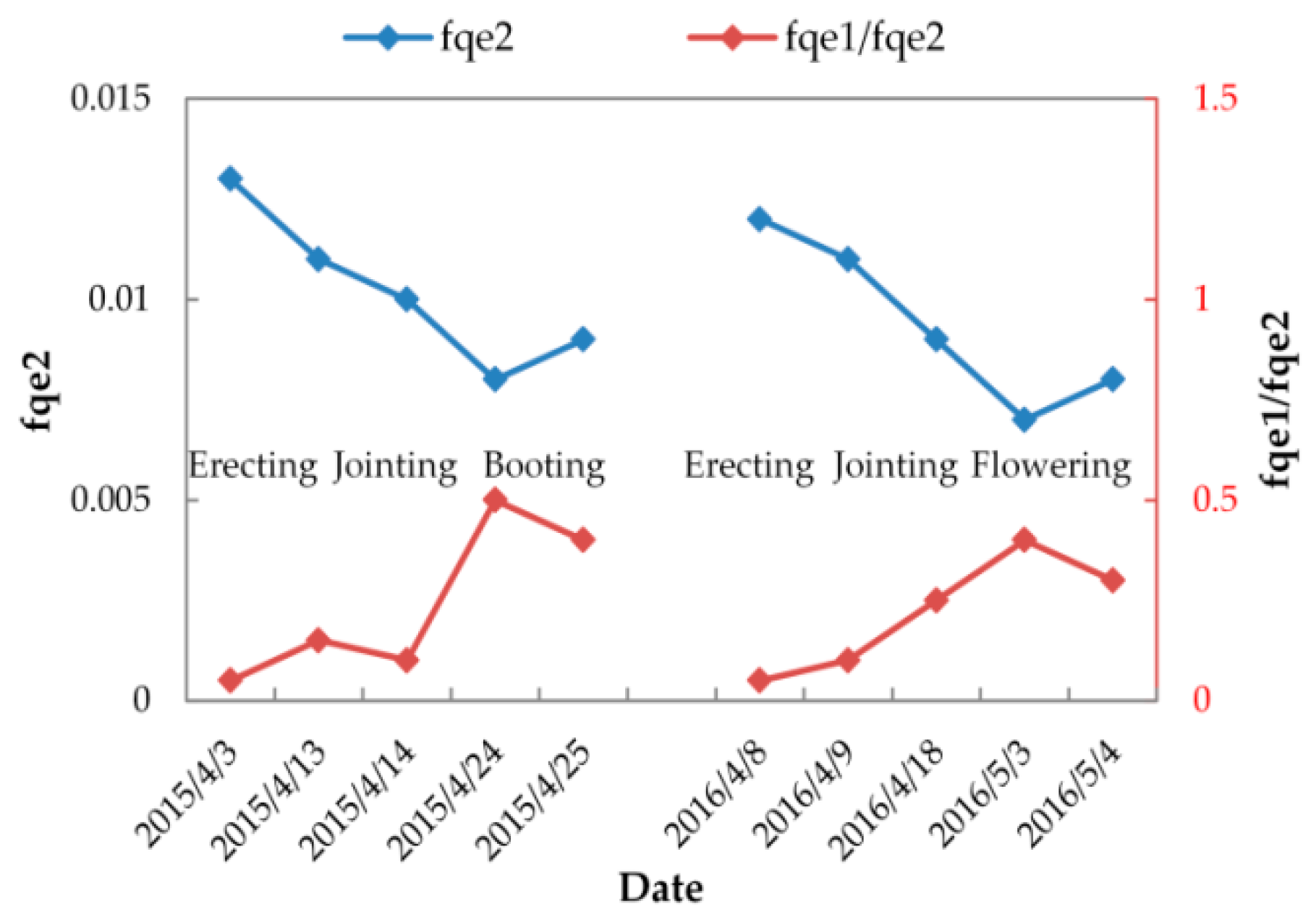
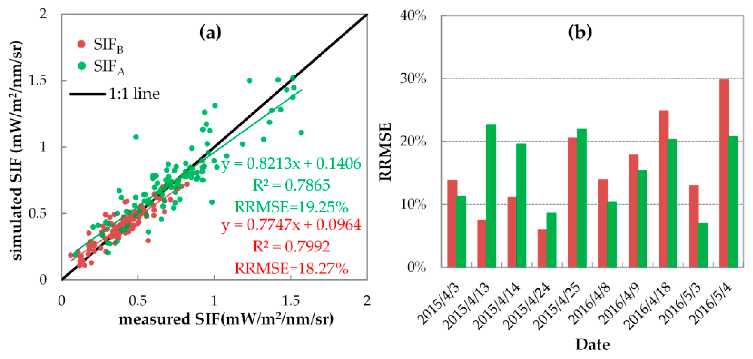
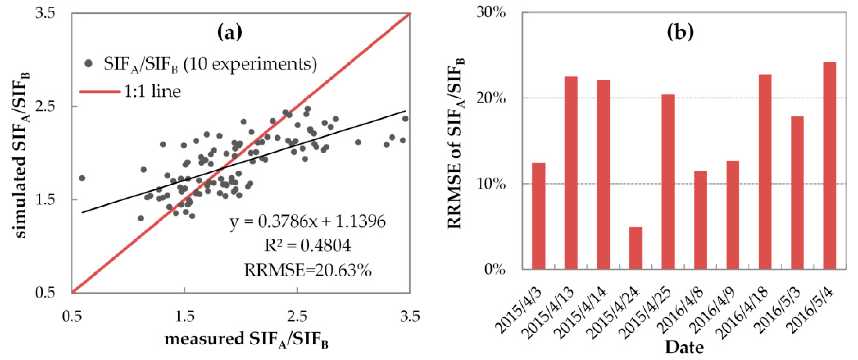
Table 1.
Values or sources of the main input parameters of the SCOPE model used in our simulation
| Parameters | Definition | Unit | Value/Source |
|---|---|---|---|
| Leaf biochemistry | |||
| Vcmo | Maximum carboxylation capacity at 25 °C | μmol m−2 s−1 | Inversion |
| m | Ball-berry stomatal conductance parameter | — | 9 |
| Rdparam | Parameter for dark respiration (Rd = Rdparam × Vcmo) | — | 0 |
| Leaf optical | |||
| Cab | Chlorophyll content density | μg/cm2 | Measurement |
| Cw | Leaf equivalent water thickness | cm | Measurement |
| Cdm | Dry matter content | g/cm2 | Measurement |
| N | Leaf thickness parameters | — | 1.4 |
| Canopy | |||
| LAI | Leaf area index | m2/m2 | Measurement |
| LIDFa | LIDF parameter a, which controls the average leaf scope | — | Inversion |
| LIDFb | LIDF parameter b, which controls the distribution’s bimodality | — | −0.15 |
| Fluorescence | |||
| fqe2 | Fluorescence efficiency for PSII in dark-adapted condition | — | 0.01 or adjusted |
| fqe1/fqe2 | Ratio of fqe1 to fqe2 | — | 0.2 or adjusted |
| Meteorology | |||
| Rin | Broadband incoming shortwave radiation (0.4–2.5 μm) | W/m2 | Measurement |
| Ta | Air temperature | T | Measurement |
| p | Air pressure | hPa | Measurement |
| ea | Atmospheric vapor pressure | hPa | Measurement |
| u | Wind speed at measurement height | m/s | Measurement |
| Ca | Atmospheric CO2 concentration | ppm | Measurement |
| Geometry | |||
| LAT | Latitude | degree | Measurement |
| LON | Longitude | degree | Measurement |
| VZA | Observation zenith angle | degree | 0 |
Table 2.
The growth stages and vegetation parameters of winter wheat at the time of ten diurnal experiments in 2015 and 2016.
Table 2.
The growth stages and vegetation parameters of winter wheat at the time of ten diurnal experiments in 2015 and 2016.
| 2015 | 2016 | |||||
|---|---|---|---|---|---|---|
| April 3 | April 13 & 14 | April 24 & 25 | April 8 & 9 | April 18 | May 3 & 4 | |
| Growth stage | Erecting | Jointing | Booting | Erecting | Jointing | Flowering |
| LAI | 1.5 | 2.1 | 2.4 | 2.5 | 2.9 | 1.9 |
| Cab (μg/cm2) | 59.2 | 62.2 | 61.3 | 55.3 | 53.7 | 57.3 |
| Cw (cm) | 0.0138 | 0.0126 | 0.0158 | 0.0163 | 0.0199 | 0.0177 |
| Cdm (g/cm2) | 0.0042 | 0.0040 | 0.0045 | 0.0048 | 0.0049 | 0.0043 |
Table 3.
The retrieved daily LIDFa and Vcmo values (unit: μmol m−2 s−1) on ten fieldwork days in 2015 and 2016.
Table 3.
The retrieved daily LIDFa and Vcmo values (unit: μmol m−2 s−1) on ten fieldwork days in 2015 and 2016.
| 2015 | 2016 | |||||||||
|---|---|---|---|---|---|---|---|---|---|---|
| April 3 | April 13 | April 14 | April 24 | April 25 | April 8 | April 9 | April 18 | May 3 | May 4 | |
| LIDFa | −0.975 | −0.875 | −0.875 | −0.625 | −0.625 | −0.875 | −0.875 | −0.75 | −0.85 | −0.85 |
| Vcmo | 50 | 80 | 80 | 110 | 110 | 45 | 55 | 65 | 95 | 100 |
Table 4.
The relative root mean square error (RRMSE) and bias of diurnal SIF simulations with fixed FQE at O2-B and O2-A bands on ten fieldwork days.
Table 4.
The relative root mean square error (RRMSE) and bias of diurnal SIF simulations with fixed FQE at O2-B and O2-A bands on ten fieldwork days.
| Year | Date | O2-B | O2-A | ||
|---|---|---|---|---|---|
| RRMSE | bias | RRMSE | bias | ||
| 2015 | April 3 | 25.97% | −20.35% | 11.14% | −1.74% |
| April 13 | 12.47% | −10.78% | 22.64% | −1.96% | |
| April 14 | 12.13% | 0.71% | 28.30% | 18.29% | |
| April 24 | 13.43% | 12.62% | 22.30% | −22.24% | |
| April 25 | 24.54% | 13.47% | 26.43% | −13.85% | |
| 2016 | April 8 | 20.23% | −13.70% | 12.07% | 6.93% |
| April 9 | 19.53% | −5.83% | 18.77% | 12.43% | |
| April 18 | 29.54% | 12.99% | 21.69% | 5.58% | |
| May 3 | 40.13% | 38.16% | 8.94% | 6.43% | |
| May 4 | 38.67% | 27.79% | 23.51% | 10.84% | |
| all ten days | 24.35% | — | 23.67% | — | |
Table 5.
The simulated and measured ratio of daily SIFA and SIFB averages, as well as the relative error (RE) between them with fixed FQE for ten fieldwork days in 2015 and 2016.
Table 5.
The simulated and measured ratio of daily SIFA and SIFB averages, as well as the relative error (RE) between them with fixed FQE for ten fieldwork days in 2015 and 2016.
| 2015 | 2016 | |||||||||
|---|---|---|---|---|---|---|---|---|---|---|
| April 3 | April 13 | April 14 | April 24 | April 25 | April 8 | April 9 | April 18 | May 3 | May 4 | |
| simulated | 1.690 | 1.853 | 1.857 | 1.705 | 1.698 | 1.885 | 1.916 | 1.859 | 1.705 | 1.732 |
| measured | 1.370 | 1.686 | 1.590 | 2.470 | 2.237 | 1.522 | 1.605 | 1.990 | 2.213 | 1.997 |
| RE | 23.37% | 9.88% | 16.80% | −30.95% | −24.08% | 23.90% | 19.39% | −6.56% | −22.97% | −13.26% |
Table 6.
The variable fqe2 and fqe1/fqe2 values on ten fieldwork days in 2015 and 2016.
| 2015 | 2016 | |||||||||
|---|---|---|---|---|---|---|---|---|---|---|
| April 3 | April 13 | April 14 | April 24 | April 25 | April 8 | April 9 | April 18 | May 3 | May 4 | |
| fqe2 | 0.013 | 0.011 | 0.01 | 0.008 | 0.009 | 0.012 | 0.011 | 0.009 | 0.007 | 0.008 |
| fqe1/fqe2 | 0.05 | 0.15 | 0.1 | 0.5 | 0.4 | 0.05 | 0.1 | 0.25 | 0.4 | 0.3 |
© 2018 by the authors. Licensee MDPI, Basel, Switzerland. This article is an open access article distributed under the terms and conditions of the Creative Commons Attribution (CC BY) license (http://creativecommons.org/licenses/by/4.0/).
Share and Cite
MDPI and ACS Style
Hu, J.; Liu, X.; Liu, L.; Guan, L. Evaluating the Performance of the SCOPE Model in Simulating Canopy Solar-Induced Chlorophyll Fluorescence. Remote Sens. 2018, 10, 250. https://doi.org/10.3390/rs10020250
AMA Style
Hu J, Liu X, Liu L, Guan L. Evaluating the Performance of the SCOPE Model in Simulating Canopy Solar-Induced Chlorophyll Fluorescence. Remote Sensing. 2018; 10(2):250. https://doi.org/10.3390/rs10020250
Chicago/Turabian StyleHu, Jiaochan, Xinjie Liu, Liangyun Liu, and Linlin Guan. 2018. "Evaluating the Performance of the SCOPE Model in Simulating Canopy Solar-Induced Chlorophyll Fluorescence" Remote Sensing 10, no. 2: 250. https://doi.org/10.3390/rs10020250
Note that from the first issue of 2016, this journal uses article numbers instead of page numbers. See further details here.