Estimation of High Spatial-Resolution Clear-Sky Land Surface-Upwelling Longwave Radiation from VIIRS/S-NPP Data


1
State Key Laboratory of Remote Sensing Science, Jointly Sponsored by Beijing Normal University and Institute of Remote Sensing and Digital Earth of Chinese Academy of Sciences, Beijing 100875, China
2
Institute of Remote Sensing Science and Engineering, Faculty of Geographical Science, Beijing Normal University, Beijing 100875, China
3
U. S. Department of Agriculture, Agricultural Research Service, Hydrology and Remote Sensing Laboratory, Beltsville, MD 20705, USA
*
Author to whom correspondence should be addressed.
Remote Sens. 2018, 10(2), 253; https://doi.org/10.3390/rs10020253
Submission received: 12 December 2017
/
Revised: 29 January 2018
/
Accepted: 2 February 2018
/
Published: 7 February 2018
(This article belongs to the Special Issue Advances in Quantitative Remote Sensing in China – In Memory of Prof. Xiaowen Li)
Abstract
:Surface-upwelling longwave radiation (LWUP) is an important component of the surface radiation budget. Under the general framework of the hybrid method, the linear models and the multivariate adaptive regression spline (MARS) models are developed to estimate the 750 m instantaneous clear-sky LWUP from the top-of-atmosphere (TOA) radiance of the Visible Infrared Imaging Radiometer Suite (VIIRS) channels M14, M15, and M16. Comprehensive radiative transfer simulations are conducted to generate a huge amount of representative samples, from which the linear model and the MARS model are derived. The two models developed are validated by the field measurements collected from seven sites in the Surface Radiation Budget Network (SURFRAD). The bias and root-mean-square error (RMSE) of the linear models are −4.59 W/m2 and 16.15 W/m2, whereas those of the MARS models are −5.23 W/m2 and 16.38 W/m2, respectively. The linear models are preferable for the production of the operational LWUP product due to its higher computational efficiency and acceptable accuracy. The LWUP estimated by the linear models developed from VIIRS is compared to that retrieved from the Moderate Resolution Imaging Spectroradiometer (MODIS). They agree well with each other with bias and RMSE of −0.15 W/m2 and 25.24 W/m2 respectively. This is the first time that the hybrid method has been applied to globally estimate clear-sky LWUP from VIIRS data. The good performance of the developed hybrid method and consistency between VIIRS LWUP and MODIS LWUP indicate that the hybrid method is promising for producing the long-term high spatial resolution environmental data record (EDR) of LWUP.
1. Introduction
The surface radiation budget (SRB) is an important indicator in the study of climate formation and change and environmental prediction, which plays a key role in the global matter, energy cycles and interactions between the surface and the atmosphere system [1,2,3]. SRB is dominated by longwave radiation in the night and during most of the year in the polar regions [4,5]. Surface-upwelling longwave radiation (LWUP, 4.0–100 μm), the sum of thermal radiation emitted by the surface and reflected atmospheric downward longwave radiation, is the main cause of surface cooling in the clear night sky and is also an indirect indicator of surface temperature [5]. An accurate estimate of LWUP is one of the prerequisites for obtaining accurate weather forecasts, climate simulations, and land-surface process simulations.
Generally, we can obtain the LWUP using three approaches: field measurement, satellite remote sensing and model prediction. LWUP can be accurately measured with field instruments. However, field networks are sparsely distributed globally. Furthermore, field measurement can only represent a limited area. The spatial resolution of model prediction is relatively coarse [6]. Remote sensing can provide various kinds of products with global coverage and horizontal spatial continuity, but the temporal resolution is always limited. High spatial-resolution LWUP is an important diagnostic parameter for mesoscale land surface and atmosphere models [7] and can also serve as a bridge for validating coarse resolution data [8]. The Visible Infrared Imaging Radiometer Suite (VIIRS) is one of the key instruments onboard the Suomi National Polar-orbiting Partnership (S-NPP) satellite system and was successfully launched in 2011. The spatial resolution of VIIRS thermal-infrared channels is 750 m. Ignoring the relatively low temporal resolution of VIIRS, it is the preferred data source for estimating high spatial-resolution LWUP.
Over the past few decades, substantial efforts have been devoted to estimating LWUP at the surface using remotely sensed observations from space-borne platforms. These methods can be primarily divided into two categories: the temperature-emissivity method [7,8,9,10] and the hybrid method [11,12,13]. Current operational satellite land-surface temperature and emissivity products facilitate the estimation of LWUP [14,15,16,17], but the large uncertainties in the land-surface temperature and emissivity products limit its accuracy [18,19]. For example, the study of Wang et al. indicated that the accuracy of the temperature-emissivity method is much lower than that of the hybrid method [7]. As shown in Figure 1, the weighting function of thermal infrared channels located in narrow bands that are semi-transparent to atmospheric gases and thus sensitive primarily to emission from the surface (“atmospheric windows”) peaks at the surface and contains the surface-emission information, so LWUP can be derived from top-of-atmosphere (TOA) radiance or brightness temperature directly [13,20]. The hybrid method links the thermal-infrared TOA radiances or brightness temperatures with LWUP through comprehensive radiative transfer modeling and statistical regression. It is physically based and at the same time has a high computational efficiency. Furthermore, it can bypass the problem of temperature and emissivity separation and achieve an acceptable accuracy in practice. The hybrid method has been successfully used to produce high spatial-resolution regional [7,11,21] and global [12] LWUP recently.
VIIRS was developed based on the heritage of Moderate Resolution Imaging Spectroradiometer (MODIS) instruments and has become a key bridge to ensure long-term continuity of the environmental data records (EDRs). VIIRS provides a large number of EDRs, including aerosol optical thickness [22], vegetation index [23], land-surface albedo [24], land-surface temperature [25], sea-surface temperature [26], etc. To our knowledge, an operational LWUP product from VIIRS is not available at regional and global scales. VIIRS do not provide operational products of surface broadband emissivity (BBE) and surface downward longwave radiation. Thus, it is difficult to calculate the LWUP with the temperature-emissivity method. In addition, no operational algorithm that can be used to retrieve LWUP from VIIRS has been reported in the literature.
We have developed a hybrid method for retrieving clear-sky LWUP from MODIS data and produced two years’ global LWUP product recently [12]. It is possible to produce long-term high spatial-resolution EDR of LWUP by combining MODIS and VIIRS. The first step is to develop a hybrid method to estimate the global 750-m instantaneous clear-sky LWUP from VIIRS data. The article is arranged as follows. The data including satellite data, field measurements, and atmospheric profiles are described in Section 2. The method and validation results are provided in Section 3 and Section 4. A brief discussion and conclusion are given in Section 5 and Section 6.
2. Data
2.1. Visible Infrared Imaging Radiometer Suite (VIIRS) Data
VIIRS has been developed based on the heritage of legacy instruments, including AVHRR and MODIS, and extends and improves on them [27]. The VIIRS has 22 spectral channels with wavelengths ranging from 0.41 μm to 12.5 μm, which can be used for environmental monitoring and numerical weather forecasting. The on-orbit verification and intensive calibration and validation using a ground target show that VIIRS is working very well [28,29]. More than 20 environmental data records have been produced operationally from VIIRS data, including clouds, land-surface temperature and sea-surface temperature, vegetation index, aerosol optical thickness, active fire, snow/ice, surface albedo, etc.
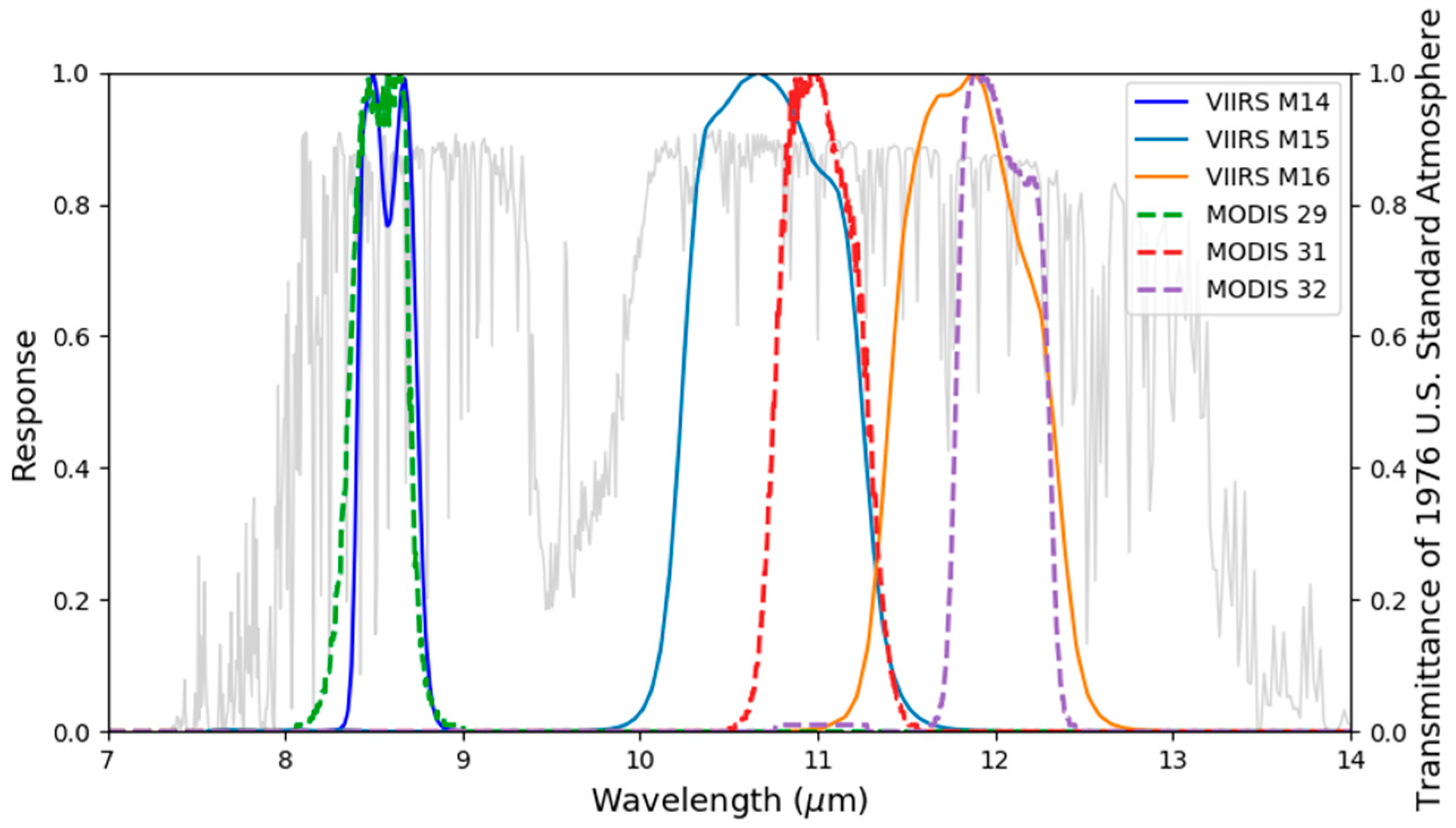
The VIIRS data utilized in this study include the VIIRS sensor data records (SDR) and VIIRS Cloud Mask intermediate product (VCM). The VIIRS SDR contains the day–night band, imagery band, moderate resolution band and geolocation data. Three thermal-infrared channels, M14, M15 and M16, which are located in the “atmospheric windows” and are sensitive to the LWUP, are finally selected. These three channels have similar channel characteristics to MODIS channels 29, 31 and 32. The relative spectral responses of VIIRS channels M14, M15 and M16 as well as MODIS channels 29, 31 and 32 are displayed in Figure 1. The VIIRS VCM product is used to identify whether a pixel is clear-sky or cloudy [30]. The pixels with confident clear flag are identified as clear-sky pixels. In addition, the longitude, latitude and the sensor view zenith angle data are also provided in the SDR.
2.2. Atmospheric Profiles
In this study, two years of the Atmospheric Infrared Sounder (AIRS) level 2 standard atmospheric profiles are collected to construct the atmospheric profile database. Launched aboard the Earth Observing System (EOS) second satellite Aqua, the AIRS instrument has 2378 infrared spectral channels covering 3.74–15.39 μm with a high spectral resolution (λ/Δλ) of 1200 [31]. The AIRS infrared band is very stable, and the offset is less than 10 mK/yr [32]. The accuracy of temperature measurement of AIRS is better than 250 mK, and the absolute calibration accuracy of most bands can reach 100 mK. It is the most accurate and stable hyperspectral infrared detector up until now (http://daac.gsfc.nasa.gov/AIRS/). AIRS can be used to obtain the global atmospheric three-dimensional physical state (atmospheric temperature, water vapor, clouds, etc.) and the distribution of trace gases (ozone, carbon dioxide and methane, etc.) daily [33]. The temperature profile of AIRS has 28 layers, and the corresponding atmospheric pressure varies from 1100 hPa to 0.1 hPa. Meanwhile, the AIRS water-vapor profile has 14 layers, and the corresponding atmospheric pressure ranges from 1100 hPa to 50 hPa.
2.3. Surface Radiation Budget Network (SURFRAD)
The Surface Radiation Budget Network (SURFRAD) network was established in 1993 to supply accurate, longstanding and persistent measurements of the surface radiation budget for climate change studies [34]. SURFRAD provides quality-controlled field measurements including downward and upwelling solar irradiance and longwave infrared irradiation, along with other meteorological observations, such as wind speed, atmospheric pressure and relative humidity, etc. SURFRAD measurements are widely used for the validation of satellite-derived products and the details about the SURFRAD site and related instruments can be found in [34]. Daily one or three-minute SURFRAD data are organized into daily ASCII text and can be freely downloaded from ftp://aftp.cmdl.noaa.gov/data/radiation/surfrad. In addition, the basic data are routinely sent to several archives including the World Radiation Data Center (WRDC), National Climatic Data Center (NCDC), and Baseline Surface Radiation Network (BSRN). The location, elevation and land cover of the seven SURFRAD sites are listed in Table 1.
Site upwelling and downward thermal infrared irradiance are measured using two precision infrared radiometers (PIR). The PIRs are sensitive to the spectral range from 3 µm to 50 µm. Three standard PIRs, which are annually calibrated by world-reputable organizations, are used to calibrate these two PIRs adopted in SURFRAD network. The spectral range of the measurements can be extended to 4–100 µm by calibration [35]. The overall accuracy of PIR ground measurement is approximately ±9 W/m2 [34], and is reported to be about ±5 W/m2 recently [36]. The VIIRS moderate resolution band (M-band) has a resolution of 750 m at nadir. The spatial matching issue and scale effect need be considered when validating satellite-derived LWUP using SURFRAD ground measurements. The footprint of SURFRAD PIRs is much smaller compared to that of the VIIRS. Fortunately, SURFRAD sites were selected at the locations where the surrounding land cover of the site was homogeneous. For example, Wang et al. [7] compared the brightness temperature of the ASTER pixel that contains the SURFRAD site to other neighboring pixels within 1 km × 1 km and 2 km × 2 km windows. They found that the discrepancies between the central pixel and surrounding pixels were less than 1 K in general, and the standard deviations of center pixel and surrounding pixels were less than 2 K under most conditions. Therefore, the SURFRAD measurements were used to validate the derived VIIRS LWUP directly.
3. Method
As shown in Figure 1, the channel characteristics of VIIRS channels M14, M15 and M16 are similar to those of MODIS channels 29, 31, and 32, which have been successfully used to derive LWUP using hybrid method at regional and global scales [7,12]. In this section, we developed the hybrid method for VIIRS using TOA radiance of channels M14, M15 and M16 under the general framework of the hybrid method. First, a huge amount of representative samples are generated by extensive radiative transfer modeling; then the linear model and MARS model are established to predict LWUP using TOA radiance of channels M14, M15 and M16.
3.1. Radiative Transfer Modeling
The surface upwelling longwave radiation consists of two components: longwave radiation emitted by the surface and surface-reflected atmospheric downward longwave radiation, which can be written as:
where the is the surface broadband emissivity. is the surface temperature. is the downward longwave radiation. and are the spectral integration range (4–100 μm).
A representative simulation database is required to train the hybrid method, such as the linear model and the MARS model. The moderate resolution atmospheric transmission (MODTRAN) software [37], which is widely used by researchers all over the world, can be used to simulate the radiation transmission and interaction between the atmosphere and the land surface under various atmospheric and surface conditions. Allowing for the difference between land-surface temperature and atmospheric temperature, the global land surface is divided into three regions: the low-latitude region (30°S–30°N), middle-latitude region (30°S–60°S, 30°N–60°N), high-latitude region (60°S–90°S, 60°N–90°N) [12]. At the same time, the atmospheric profiles are also divided into these three categories according to the latitude. For each sub-region, we extracted the atmospheric profiles from AIRS Level 2 standard atmosphere product and constructed the atmospheric profile database. To avoid excessive computation and to alleviate the similarity of the profiles, a screening process was applied, and the criteria proposed in [12] adopted to measure the similarity of atmospheric profiles. In total, 2842, 35,487 and 41,724 atmospheric profiles of high-latitude, mid-latitude and low-latitude region were obtained. MODTRAN 5.2 was used to simulate the spectral downward longwave radiance, thermal path radiance and spectral transmittance for each atmospheric profile and sensor view zenith angle. During the simulation, the sensor view zenith angles were set from 0° to 60° with an interval of 15°. We calculated the difference between surface temperature and the bottom layer temperature of atmospheric profiles for each region using two-year AIRS standard L2 product. The surface temperature was determined based on this difference. For example, the surface temperature of mid-latitude is equal to the bottom layer temperature plus a range of [−10, 15] K with a step of 5 K. Eighty-four representative spectral emissivity spectra including vegetation, soil, snow/ice, water selected from ASTER spectral library [38] and MODIS UCSB spectral library [39] and their combinations were used to characterize the land-surface conditions. Since there was no spectral emissivity value for wavelengths larger than 14 μm, the emissivity value was supposed to be the same as that at wavelength 14 μm in the following simulations. When the surface and atmospheric parameters were determined, the VIIRS TOA channel radiances are calculated using the following simplified equation:
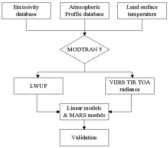
where is the TOA radiance for channel M14, M15 and M16 of VIIRS; and are path thermal radiance and spectral downward longwave radiance, respectively; is the spectral response function for channels M14, M15 and M16; and are the spectral range of VIIRS TIR channel. The flowchart of the hybrid method is displayed in Figure 2.
3.2. Linear Model
A linear model with the following expression was developed using the generated samples in Section 3.1:
where , , and are coefficients; and M14, M15 and M16 are TOA radiance for moderate resolution bands 14, 15 and 16 of the VIIRS. The linear model is fitted for each sub-region and view zenith angle.
3.3. The Multivariate Adaptive Regression Spline (MARS) Model
To probe the non-linear relationship between TOA spectral radiance and LWUP, we also use the multivariate adaptive regression spline (MARS) to model the non-linear relationship between TOA spectral radiance and LWUP with the same samples as those used by the linear model. MARS was proposed by Jerome H. Friedman in 1991 [40]. MARS is a highly generalized and highly specialized regression method for high-dimensional data. The regression method takes the tensor product of spline functions as the basis functions, while the determination of the basis functions and their number are automatically completed by the data without manual selection. In the multi-dimensional case, how to divide the space has become a critical problem, but the MARS model can solve this problem well. The MARS model is defined as follows:
where is the basis function; is coefficient; is the coefficient of the basis function; M is the number of the basis function; is the number of knots in the basis function; is 1 or −1, and indicates the spline function on the right or left side; labels the independent variables; and is a knot location. The basis function of MARS is a single spline function, or is the result of the interaction of multiple spline functions. The spline functions on the right and left sides are defined as follows:
where t is the position of the node; and are used to describe spline functions on the right and left regions when t is given; q is the power (>0) to which the splines are raised; and “+” takes 0 for negative values.
MARS is built in two phases: the forward-basis function selection and backward-pruning process. In the first stage, MARS begins with just the intercept term and iterations are conducted to add pairs of basis functions, which can minimize the training error to the utmost extent. In order to avoid overfitting, a backward-pruning process is needed. In the backward-pruning phase, the basis function, which contributes the least to the reduction of training error, is deleted at a time. The model with the lowest GCV (generalized cross-validation) is finally selected. The GCV, as an estimator for effective mean residual error, can achieve a balance between goodness of fit and model complexity. The GCV is calculated as follows:
where N is the number of samples in the training data; is the estimation of ; and enp is the effective number of parameters:
where c is the penalty parameter; and k is the number of non-constant basis functions.
The training of MARS is based on the ARESLab package of the MATLAB platform, in which the MARS is implemented according to Friedman’s original papers [40] and all parameters in the ARESLab package are automatically determined. The source code of the ARESLab toolbox can be downloaded from the following website: www.cs.rtu.lv/jekabsons/regression.html.
4. Results
4.1. Training Results of the Linear Model and MARS Model
The linear model can account for more than 97.7%, 98.5% and 99.1% of the variation of the LWUP in the simulation database for the low-latitude, middle-latitude and high-latitude regions, respectively. The bias is zero, and the RMSE ranges from 5.27 to 13.02 W/m2. The RMSE in the low-latitude region is larger than that in the middle-latitude and high-latitude region. In addition, the RMSE for the larger view zenith angle is greater than that with the smaller view zenith angle. Details about fitting the results of the linear models can be found in Table 2.
The training results of the MARS model are also displayed in Table 2. The MARS model can account for more than 98.2%, 98.7% and 99.2% of the variation in the simulation database for the low-latitude, middle-latitude and high-latitude regions, respectively. The biases of all MARS models are zero, and the RMSEs range from 8.53 to 10.13 W/m2, 6.64 to 8.24 W/m2, and 4.8 to 6.47 W/m2 for the low-latitude, middle-latitude and high-latitude regions, respectively. The RMSEs of the MARS models are slightly less than those of the linear models.
4.2. Validation with Field Measurements
4.2.1. The Linear Model
The field measurements collected from the SURFRAD network were used to validate the linear models developed. When the view zenith angle was not equal to 0°, 15°, 30°, 45°, 60°, LWUP was linearly interpolated from LWUPs predicted by the linear model with an adjacent view zenith angle. View zenith angle exceeding 60° was not considered. The cloud-mask information was extracted from the VIIRS Cloud Mask intermediate product. Clear sky was identified when 3 × 3 neighboring pixels of the site are clear to ensure that the field measurements at the site were not affected by clouds and cloud shadows. In total, 2901 validation samples were finally obtained.
Figure 3 shows the comparison between the estimated LWUP and the ground measurements. We can find that the average bias and RMSE are −4.59 and 16.15 W/m2, respectively, at seven SURFRAD sites. For further analysis, the validation samples were divided into two groups: daytime and night time according to the local solar time. The bias ranged from −16.94 to 7.84 W/m2, and RMSE ranges from 13.84 to 30.43 W/m2 in the daytime. The average bias and RMSE were −1.40 W/m2 and 21.57 W/m2. If Desert_Rock_NVt is not considered, the average bias and RMSE were −1.12 W/m2 and 21.71 W/m2. During the night time, the bias ranged from −20.48 W/m2 to 2.97 W/m2, and RMSE ranged from 8.76 W/m2 to 21.22 W/m2. The average bias and RMSE were −8.3 W/m2 and 13.46 W/m2. If Desert_Rock_NVt is not considered, the average bias and RMSE were −5.33 W/m2 and 10.73 W/m2. The LWUP estimated at night was less divergent than that in the daytime.
4.2.2. MARS Models
The LWUP estimated by MARS models was validated with the same ground measurements. As shown in Figure 4, we can find that the average bias and RMSE were −5.23 and 16.38 W/m2. The bias ranged from −16.15 to 8.15 W/m2, and RMSE ranged from 12.12 to 29.96 W/m2 in the daytime. The average bias and RMSE were −1.27 W/m2 and 19.79 W/m2. If Desert_Rock_NVt is not considered, the average bias and RMSE were −1.13 W/m2 and 21.64 W/m2. During the nighttime, the bias ranged from −20.46 W/m2 to 2.25 W/m2, and RMSE ranged from 8.66 W/m2 to 15.26 W/m2. The average bias and RMSE were −8.93 W/m2 and 13.8 W/m2. If Desert_Rock_NVt is not considered, the average bias and RMSE were −5.93 W/m2 and 11.03 W/m2. The distribution of the points in Figure 4 is similar to that in Figure 3.
Regarding the satellite-derived surface radiative fluxes, an accuracy of approximately ±20 W/m2 for instantaneous footprint values is required by the hydrological, meteorological, and agricultural research communities [41]. According to the validation results in this study, both the linear and MARS models can meet this requirement. Overall, the linear models are slightly better than the MARS models, although MARS can model the non-linearity between LWUP and TOA spectral radiance well during the training stage. Two reasons may account for this phenomenon. First, the zenith angles of the validation samples are all less than 40°, and the differences between the linear models and the MARS models are slight when the zenith angle is less than 45°, as shown in Table 2. Second, various kinds of satellite measurement errors are likely to be magnified by the non-linear model such as MARS. Due to the higher computational efficiency of the linear models, it is more adaptable to produce operational LWUP product.
A few studies have been devoted to estimating high spatial-resolution LWUP from MODIS and VIIRS. For example, Wang et al. [7] developed the linear models for estimating North American LWUP using MODIS data. The average bias and RMSE over SURFRAD site were −10.97 W/m2 and 18.35 W/m2. Jiao et al. [11] developed the neural network models for estimating LWUP from MODIS and VIIRS data over the Tibet Plateau. The average bias and RMSE of the validation results for MODIS were 11.24 W/m2 and 26.78 W/m2. The accuracy of LWUP from VIIRS was not validated. Cheng and Liang developed the linear models for estimating LWUP from MODIS data at global scale. The bias and RMSE of the validation over SURFRAD site were −4.49 W/m2 and 13.47 W/m2. Compared to these studies, the accuracies of the newly developed hybrid method are comparable or superior to those of the related published references.
4.3. Comparison between Moderate Resolution Imaging Spectroradiometer (MODIS) and VIIRS Surface-Upwelling Longwave Radiation (LWUP)
Remote-sensing instruments such as MODIS and VIIRS are critical for providing continual and reliable measurements of the atmosphere, ocean and land-surface variables at the global scale. Furthermore, VIIRS is developed based on the heritage of MODIS instruments and has become a key bridge to ensure long-term continuity of the climate data records. LWUP estimated from VIIRS is compared with that retrieved from MODIS using the linear models of Cheng et al. [12] to check the consistency between the two instruments. The overpass time of the MODIS granule image is at 20:40 (UTC), 17 August 2014 and the VIIRS granule image is acquired from 20:46 to 20:51 (UTC) on the same day. The time difference between the two images is less than 10 min. Therefore, it is supposed that there are no significant differences in atmospheric conditions and land-surface properties within the 10-min period. In addition, the corresponding MOD35 and VIIRS Cloud Mask intermediate products are used to eliminate the influence of clouds. The linear hybrid method proposed by Cheng et al. [12] is used to calculate the LWUP from MODIS data, which has been validated by three measurement networks with a bias and RMSE of −0.31 W/m2 and 19.92 W/m2 in total.
The VIIRS image was aggregated to 1 km with bi-linear resampling method to match the spatial resolution of MODIS. The LWUP derived from both MODIS and VIIRS data were compared without considering the pixels that covered by invalid data or were contaminated by cloud. The spatial distributions of LWUP for MODIS and VIIRS are displayed in Figure 5, from which we can find that the LWUP distribution pattern of VIIRS is similar to that of the MODIS. In addition, the density plot of the LWUP is shown in Figure 6. Most of the LWUP values are concentrated between 400 and 800 W/m2 with R2 of 0.88. The bias and RMSE are −0.15 W/m2 and 25.24 W/m2, respectively. Thus, the LWUP of VIIRS is consistent with that of MODIS. This result is consistent with the study of Jiao et al. [11]. They compared the LWUP retrieved from MODIS and VIIRS at Tibet Plateau. The R2, bias and RMES were 0.52 W/m2, 2.87 W/m2 and 26.02 W/m2, respectively.
5. Discussion
5.1. Cloud Effect
In Section 4, the established hybrid methods were validated by the field measurements. Generally, most of the estimated LWUPs were closer to the one-to-one line. The points were less divergent in the night time than in the daytime. This may be because that the land surface is more homogeneous in the night time than in the daytime [42]. Compared to other sites, obvious underestimation is found in the desert site. Wang and Liang [7] thought air traffic out of Los Angeles produces many cirrus clouds over this site, and cloud contamination may be a significant source of error at this site. Thus, one of the reasons may be that the VIIRS Cloud Mask intermediate product cannot identify all kinds of cloud types, especially the cirrus cloud.
In order to test this assumption, we downloaded three years (2014–2017) field measurements from Atmospheric Radiation Measurement (ARM) program Southern Great Plains (SGP) site C1 (https://www.arm.gov). The downloaded data include the LWUP, cloud-base height and other auxiliary data. The cloud-base height information is derived from the Micropulse Lidar (MPL). MPL is a ground-based remote-sensing instrument that can be used to measure the altitude of clouds by transmitting pulses of light and using the receiver to detect the light scattered back by clouds and precipitation. From the time delay between each outgoing pulse and the backscattered signal, the distance to the scatterer is inferred [43]. The VIIRS pixels are, first, identified by the VIIRS Cloud Mask intermediate product, and then the extracted clear-sky pixels are further screened by the field measurements. The pixels with more than one detected cloud base are considered as cloudy, while those with no significant backscatter detected are regarded as true clear-sky pixels. The developed liner models are used to retrieve LWUP. The validation results of LWUP at site C1 are displayed in Figure 7. The bias and RMSE of cloudy pixels are −6.65 W/m2 and 16.04 W/m2, while bias and RMSE of clear-sky pixels are −2.94 W/m2 and 15.62 W/m2. The VIIRS Cloud Mask intermediate product actually cannot identify all kinds of cloud types, and undetected cloud will cause the underestimation of LWUP.
5.2. Broadband Emissivity (BBE) Effect
The obvious underestimation of LWUP at Desert_Rock_NV may also be related to BBE of the surface. Taking the developed linear model for the mid-latitude region at nadir view as an example, we investigated the effects of surface BBE on the accuracy of LWUP estimation. The bias and RMSE of the fitting liner model at nadir are zero and 6.94 W/m2. We calculated the average bias and RMSE for each emissivity spectrum as well as the corresponding BBE. The relationship between BBE versus bias is shown in Figure 8; 78% samples have a negative bias when their BBE is less than 0.966 and 88% BBE has a positive bias when BBE is equal to or larger than 0.966. It is very likely to produce negative bias at Desert_Rock_NV from the point of the developed linear models, because its BBE is less than 0.966. We have also investigated the relationship between the fitting residual and land-surface temperature (LST) with the same data, and no significant overestimated or underestimated trend is found. Thus, cloud and surface BBE are two primary factors that affect the accuracy of the LWUP estimate.
6. Conclusions
LWUP is an important component of the land-surface radiation budget. We developed two hybrid methods, namely, the linear model and MARS model, to estimate the 750-m instantaneous clear-sky LWUP from the VIIRS TOA channel radiances of M14, M15, and M16 at the global scale.
To consider the difference between the land-surface temperature and air temperature, the global land surface was divided into 3 regions based on latitude. Extensive radiative transfer modeling was conducted to produce a huge amount of representative samples for each sub region. The linear models and the MARS models were established at 0°, 15°, 30°, 45° and 60° viewing zenith angles for each sub region. According to the statistical results, the linear models can account for more than 97.7% of the variation in the simulation database, the bias is zero, and the RMSEs range from 5.27 to 13.02 W/m2; the MARS models can account for more than 98.2% of the variation in the simulation database, the bias is zero, and the RMSEs range from 4.8 to 10.13 W/m2. Then, the two models were validated using three years (2014–2017) of ground measurements collected from seven SURFRAD sites. The average bias and RMSE of the linear models were −4.59 W/m2 and 16.15 W/m2, whereas the average bias and RMSE of the MARS models were −5.23 W/m2 and 16.38 W/m2. The difference between the linear models and the MARS models was not significant. The linear models have higher computational efficiency and are easy to implement, so it is a good choice for producing the operational LWUP product. The LWUP retrieved from VIIRS by the developed linear models was compared to that retrieved from MODIS by the previous linear models developed. Their spatial distribution pattern agreed well with each other; the bias and RMSE were −0.15 W/m2 and 25.24 W/m2.
This is the first time that the hybrid method has been applied to global estimates of clear-sky LWUP from VIIRS data. Limited validation results indicate that the accuracy of the hybrid method can meet the accuracy requirement of the hydrological, meteorological, and agricultural research communities. The good performance of the developed hybrid method and consistency between VIIRS LWUP and MODIS LWUP indicate that the hybrid method shows promise for producing a long-term high spatial-resolution environmental data record (EDR) of LWUP. The field measurements used for validation are collected from the SURFRAD network, which is located in the middle-latitude region. More validation data from low-latitude and high-latitude regions with other land-cover types need to be collected for further validation in the future. Also, more extensive comparison should be conducted before the generation of LWUP EDR using MODIS and VIIRS data.
Acknowledgments
The ground data used in this study are collected from Surface Radiation Budget Network (ftp://aftp.cmdl.noaa.gov/data/radiation/surfrad) and ARM Climate Research Facility (https://www.arm.gov/data). The AIRS atmosphere profile product is downloaded from NASA (http://daac.gsfc.nasa.gov/AIRS/). The VIIRS SDR and Cloud mask product are downloaded from NOAA (https://www.class.ngdc.noaa.gov/saa/products/welcome). The source code of the ARESLab toolbox is downloaded from the website: www.cs.rtu.lv/jekabsons/regression.html. This work was partly supported by the National Natural Science Foundation of China via grant 41771365, the National Key Research and Development Program of China via grant 2016YFA0600101, and the Special Fund for Young Talents of the State Key Laboratory of Remote Sensing Sciences via grant 17ZY-02.
Author Contributions
Jie Cheng conceived and designed the algorithm; Jie Cheng and Shugui Zhou performed the algorithm and analyzed the data; Shugui Zhou wrote the paper. Both authors participated in the editing of the paper.
Conflicts of Interest
The authors declare no conflicts of interest.
References
- Diak, G.R.; Mecikalski, J.R.; Anderson, M.C.; Norman, J.M.; Kustas, W.P.; Torn, R.D.; DeWolf, R.L. Estimating land surface energy budgets from space: Review and current efforts at the university of wisconsin—madison and usda–ars. Bull. Am. Meteorol. Soc. 2004, 85, 65–78. [Google Scholar] [CrossRef]
- Ellingson, R.G. Surface longwave fluxes from satellite observations: A critical review. Remote Sens. Environ. 1995, 51, 89–97. [Google Scholar] [CrossRef]
- Schmetz, J. Towards a surface radiation climatology: Retrieval of downward irradiances from satellites. Atmos. Res. 1989, 23, 287–321. [Google Scholar] [CrossRef]
- Curry, J.A.; Schramm, J.L.; Rossow, W.B.; Randall, D. Overview of arctic cloud and radiation characteristics. J. Clim. 1996, 9, 1731–1764. [Google Scholar] [CrossRef]
- Mlynczak, P.E.; Smith, G.L.; Wilber, A.C.; Stackhouse, P.W. Annual cycle of surface longwave radiation. J. Appl. Meteorol. Climatol. 2011, 50, 1212–1224. [Google Scholar] [CrossRef]
- Ma, Q.; Wang, K.; Wild, M. Evaluations of atmospheric downward longwave radiation from 44 coupled general circulation models of cmip5. J. Geophys. Res. Atmos. 2014, 119, 4486–4497. [Google Scholar] [CrossRef]
- Wang, W.; Liang, S.; Augustine, J.A. Estimating high spatial resolution clear-sky land surface upwelling longwave radiation from modis data. IEEE Trans. Geosci. Remote Sens. 2009, 47, 1559–1570. [Google Scholar] [CrossRef]
- Bisht, G.; Venturini, V.; Islam, S.; Jiang, L. Estimation of the net radiation using modis (moderate resolution imaging spectroradiometer) data for clear sky days. Remote Sens. Environ. 2005, 97, 52–67. [Google Scholar] [CrossRef]
- Long, D.; Gao, Y.; Singh, V.P. Estimation of daily average net radiation from modis data and dem over the baiyangdian watershed in north china for clear sky days. J. Hydrol. 2010, 388, 217–233. [Google Scholar] [CrossRef]
- Wang, C.; Tang, B.-H.; Huo, X.; Li, Z.-L. New method to estimate surface upwelling long-wave radiation from modis cloud-free data. Opt. Express 2017, 25, A574–A588. [Google Scholar] [CrossRef] [PubMed]
- Jiao, Z.; Yan, G.; Zhao, J.; Wang, T.; Chen, L. Estimation of surface upward longwave radiation from modis and viirs clear-sky data in the tibetan plateau. Remote Sens. Environ. 2015, 162, 221–237. [Google Scholar] [CrossRef]
- Cheng, J.; Liang, S. Global estimates for high-spatial-resolution clear-sky land surface upwelling longwave radiation from modis data. IEEE Trans. Geosci. Remote Sens. 2016, 54, 4115–4129. [Google Scholar] [CrossRef]
- Lee, H.-T.; Ellingson, R.G. Development of a nonlinear statistical method for estimating the downward longwave radiation at the surface from satellite observations. J. Atmos. Ocean. Technol. 2002, 19, 1500–1515. [Google Scholar] [CrossRef]
- Liang, S.; Zhao, X.; Liu, S.; Yuan, W.; Cheng, X.; Xiao, Z.; Zhang, X.; Liu, Q.; Cheng, J.; Tang, H. A long-term global land surface satellite (glass) data-set for environmental studies. Int. J. Digit. Earth 2013, 6, 5–33. [Google Scholar] [CrossRef]
- Cheng, J.; Liang, S.; Yao, Y.; Ren, B.; Shi, L.; Liu, H. A comparative study of three land surface broadband emissivity datasets from satellite data. Remote Sens. 2013, 6, 111–134. [Google Scholar] [CrossRef]
- Vogt, J.V. Land surface temperature retrieval from noaa avhrr data. In Advances in the Use of NOAA AVHRR Data for Land Applications; Springer: Berlin/Heidelberg, Germany, 1996; pp. 125–151. [Google Scholar]
- Wan, Z.; Dozier, J. A generalized split-window algorithm for retrieving land-surface temperature from space. IEEE Trans. Geosci. Remote Sens. 1996, 34, 892–905. [Google Scholar]
- Wan, Z.; Zhang, Y.; Zhang, Q.; Li, Z.-L. Quality assessment and validation of the modis global land surface temperature. Int. J. Remote Sens. 2004, 25, 261–274. [Google Scholar] [CrossRef]
- Cheng, J.; Liang, S.; Verhoef, W.; Shi, L.; Liu, Q. Estimating the hemispherical broadband longwave emissivity of global vegetated surfaces using a radiative transfer model. IEEE Trans. Geosci. Remote Sens. 2016, 54, 905–917. [Google Scholar] [CrossRef]
- Tang, B.; Li, Z.-L. Estimating of instananeous net surface longwave radiation from modis cloud-free data. Remote Sens. Environ. 2008, 112, 3482–3492. [Google Scholar] [CrossRef]
- Wang, T.; Yan, G.; Chen, L. Consistent retrieval methods to estimate land surface shortwave and longwave radiative flux components under clear-sky conditions. Remote Sens. Environ. 2012, 124, 61–71. [Google Scholar] [CrossRef]
- Jackson, J.M.; Liu, H.; Laszlo, I.; Kondragunta, S.; Remer, L.A.; Huang, J.; Huang, H.C. Suomi-npp viirs aerosol algorithms and data products. J. Geophys. Res. Atmos. 2013, 118, 12673–12689. [Google Scholar] [CrossRef]
- Vargas, M.; Miura, T.; Shabanov, N.; Kato, A. An initial assessment of suomi npp viirs vegetation index edr. J. Geophys. Res. Atmos. 2013, 118, 12301–312316. [Google Scholar] [CrossRef]
- Wang, D.; Liang, S.; He, T.; Yu, Y. Direct estimation of land surface albedo from viirs data: Algorithm improvement and preliminary validation. J. Geophys. Res. Atmos. 2013, 118, 12577–12586. [Google Scholar] [CrossRef]
- Yu, Y.; Privette, J.L.; Pinheiro, A.C. Analysis of the npoess viirs land surface temperature algorithm using modis data. IEEE Trans. Geosci. Remote Sens. 2005, 43, 2340–2350. [Google Scholar]
- Petrenko, B. Evaluation and selection of sst regression algorithms for jpss viirs. J. Geophys. Res. Atmos. 2014, 119, 4580–4599. [Google Scholar] [CrossRef]
- Schueler, C.F.; Clement, J.E.; Ardanuy, P.E.; Welsch, C.; DeLuccia, F.; Swenson, H. Npoess viirs sensor design overview. In Earth Observing Systems VI, Proceedings of the International Society for Optics and Photonics, San Diego, CA, USA, 29 July–4 August 2001; pp. 11–24. [Google Scholar]
- Xiong, X.; Butler, J.; Chiang, K.; Efremova, B.; Fulbright, J.; Lei, N.; McIntire, J.; Oudrari, H.; Sun, J.; Wang, Z. Viirs on-orbit calibration methodology and performance. J. Geophys. Res. Atmos. 2014, 119, 5065–5078. [Google Scholar] [CrossRef]
- Madhavan, S.; Brinkmann, J.; Wenny, B.N.; Wu, A.; Xiong, X. Evaluation of viirs and modis thermal emissive band calibration stability using ground target. Remote Sens. 2016, 8, 158. [Google Scholar] [CrossRef]
- Godin, R. Joint polar satellite system (jpss) viirs cloud mask (vcm) algorithm theoretical basis document (atbd). JPSS 2014, 474, 474-00033. [Google Scholar]
- Aumann, H.; Chanhine, M.T.; Gautier, C. Airs/amsu/hsb on the aqua mission: Design, science objectives, data products, and processing systems. IEEE Trans. Geosci. Remote Sens. 2003, 41, 253–264. [Google Scholar] [CrossRef]
- Aumann, H.; Elliott, D.; Strow, L. Validation of the radiometric stability of the atmospheric infrared sounder. In Earth Observing Systems XVII, Proceedings of the International Society for Optics and Photonics, San Diego, CA, USA, 14–16 August 2012; p. 85100T. [Google Scholar]
- Susskind, J.; Barnet, C.D.; Blaisdell, J.M. Retrieval of atmoshperic and surface parameters from airs/amsu/hsb data in the presence of clouds. IEEE Trans. Geosci. Remote Sens. 2003, 41, 390–409. [Google Scholar] [CrossRef]
- Augustine, J.A.; DeLuisi, J.J.; Long, C.N. Surfrad—A national surface radiation budget network for atmospheric research. Bull. Am. Meteorol. Soc. 2000, 81, 2341–2357. [Google Scholar] [CrossRef]
- Wang, K.; Dickinson, R.E. Global atmospheric downward longwave radiation at the surface from ground-based observations, satellite retrievals, and reanalyses. Rev. Geophys. 2013, 51, 150–185. [Google Scholar] [CrossRef]
- Augustine, J.A.; Dutton, E.G. Variability of the surface radiation budget over the united states from 1996 through 2011 from high-quality measurements. J. Geophys. Res. Atmos. 2013, 118, 43–53. [Google Scholar] [CrossRef]
- Berk, A.; Anderson, G.; Acharya, P.; Shettle, E. Modtran5. 2.0. 0 User’s Manual; Spectral Sciences Inc.: Burlington, MA, USA; Air Force Research Laboratory: Hanscom, MA, USA, 2008. [Google Scholar]
- Baldridge, A.; Hook, S.; Grove, C.; Rivera, G. The aster spectral library version 2.0. Remote Sens. Environ. 2009, 113, 711–715. [Google Scholar] [CrossRef]
- Snyder, W.C.; Wan, Z.; Zhang, Y.; Feng, Y.-Z. Classification-based emissivity for land surface temperature measurement from space. Int. J. Remote Sens. 1998, 19, 2753–2774. [Google Scholar] [CrossRef]
- Friedman, J.H. Multivariate adaptive regression splines. Ann. Stat. 1991, 1–67. [Google Scholar] [CrossRef]
- Gupta, S.K.; Kratz, D.P.; Wilber, A.C.; Nguyen, L.C. Validation of parameterized algorithms used to derive trmm–ceres surface radiative fluxes. J. Atmos. Ocean. Technol. 2004, 21, 742–752. [Google Scholar] [CrossRef]
- Wang, W.; Liang, S.; Meyers, T. Validating modis land surface temperature products using long-term nighttime ground measurements. Remote Sens. Environ. 2008, 112, 623–635. [Google Scholar] [CrossRef]
- Zhao, C.; Wang, Y.; Wang, Q.; Li, Z.; Wang, Z.; Liu, D. A new cloud and aerosol layer detection method based on micropulse lidar measurements. J. Geophys. Res. Atmos. 2014, 119, 6788–6802. [Google Scholar] [CrossRef]
Figure 1.
Relative spectral responses of Visible Infrared Imaging Radiometer Suite (VIIRS) channels M14, M15 and M16, and Moderate Resolution Imaging Spectroradiometer (MODIS) channels 29, 31 and 32. The gray line represents the transmittance of the 1976 U.S. Standard Atmosphere.
Figure 1.
Relative spectral responses of Visible Infrared Imaging Radiometer Suite (VIIRS) channels M14, M15 and M16, and Moderate Resolution Imaging Spectroradiometer (MODIS) channels 29, 31 and 32. The gray line represents the transmittance of the 1976 U.S. Standard Atmosphere.

Figure 2.
Flowchart for developing the hybrid method.

Figure 3.
Validation results of the linear model at SURFRAD sites. (a) Bondville_IL; (b) Boulder_CO; (c) Desert_Rock_NV; (d) Fort_Peck_MT; (e) Goodwin_Creek_MS; (f) Penn_State_PA; (g) Sioux_Falls_SD.
Figure 3.
Validation results of the linear model at SURFRAD sites. (a) Bondville_IL; (b) Boulder_CO; (c) Desert_Rock_NV; (d) Fort_Peck_MT; (e) Goodwin_Creek_MS; (f) Penn_State_PA; (g) Sioux_Falls_SD.

Figure 4.
Validation results of the MARS model at SURFRAD sites. (a) Bondville_IL. (b) Boulder_CO. (c) Desert_Rock_NV. (d) Fort_Peck_MT. (e) Goodwin_Creek_MS. (f) Penn_State_PA. (g) Sioux_Falls_SD.
Figure 4.
Validation results of the MARS model at SURFRAD sites. (a) Bondville_IL. (b) Boulder_CO. (c) Desert_Rock_NV. (d) Fort_Peck_MT. (e) Goodwin_Creek_MS. (f) Penn_State_PA. (g) Sioux_Falls_SD.


Figure 5.
Distribution of LWUPs derived from VIIRS and MODIS images.

Figure 6.
The scatterplot of retrieved LWUP from VIIRS and that retrieved from MODIS.

Figure 7.
Validation results of the linear model at the Atmospheric Radiation Measurement (ARM) program Southern Great Plains (SGP) C1 site. (a) Pixels that were identified as clear sky by the VIIRS cloud mask whereas cloudy by ground-based Lidar; (b) pixels that were identified as clear sky by both the VIIRS Cloud Mask and the Lidar.

Figure 8.
The relationships between Broadband Emissivity (BBE) versus bias of retrieved LWUP.


Table 1.
Information of sites in the Surface Radiation Budget Network (SURFRAD) network.
| Name | Location | Elevation (m) | Land Cover | Time Period of Used Data |
|---|---|---|---|---|
| Bondville_IL | 40.0519°N, 88.3731°W | 230 | Cropland | 2014–2017 |
| Boulder_CO | 40.1249°N, 105.2368°W | 1689 | Grassland | 2014–2017 |
| Desert_Rock_NV | 36.6237°N, 116.0195°W | 1007 | Desert | 2014–2017 |
| Fort_Peck_MT | 48.3078°N, 105.1017°W | 634 | Grassland | 2014–2017 |
| Goodwin_Creek_MS | 34.2547°N, 89.873°W | 98 | Grassland | 2014–2017 |
| Penn_State_PA | 40.7201°N, 77.9309°W | 376 | Cropland | 2014–2017 |
| Sioux_Falls_SD | 43.7340°N, 96.6233°W | 473 | Grassland | 2014–2017 |
Table 2.
Fitting results for the linear models and the Multivariate Adaptive Regression Spline (MARS) models.
Table 2.
Fitting results for the linear models and the Multivariate Adaptive Regression Spline (MARS) models.
| Low-Latitude Region | ||||||||||
| Linear Model | MARS | |||||||||
| Angle | a0 | a1 | a2 | a3 | R2 | Bias | RMSE | R2 | Bias | RMSE |
| 0° | 124.404 | 2.687 | 119.530 | −93.350 | 0.989 | 0.00 | 8.82 | 0.990 | 0.00 | 8.53 |
| 15° | 126.927 | 2.833 | 121.603 | −95.997 | 0.988 | 0.00 | 8.97 | 0.993 | 0.00 | 8.54 |
| 30° | 135.126 | 3.434 | 128.092 | −104.459 | 0.988 | 0.00 | 9.13 | 0.989 | 0.00 | 8.71 |
| 45° | 151.431 | 5.290 | 139.829 | −120.664 | 0.985 | 0.00 | 10.46 | 0.986 | 0.00 | 9.03 |
| 60° | 182.429 | 12.293 | 157.379 | −149.538 | 0.977 | 0.00 | 13.02 | 0.982 | 0.00 | 10.13 |
| Middle-Latitude Region | ||||||||||
| Linear Model | MARS | |||||||||
| Angle | a0 | a1 | a2 | a3 | R2 | Bias | RMSE | R2 | Bias | RMSE |
| 0° | 99.959 | 1.747 | 104.644 | −73.428 | 0.993 | 0.00 | 6.94 | 0.993 | 0.00 | 6.64 |
| 15° | 101.853 | 1.769 | 106.772 | −75.933 | 0.992 | 0.00 | 7.04 | 0.993 | 0.00 | 6.84 |
| 30° | 108.090 | 1.922 | 113.550 | −84.018 | 0.992 | 0.00 | 7.39 | 0.992 | 0.00 | 7.18 |
| 45° | 120.822 | 2.647 | 126.401 | −99.870 | 0.990 | 0.00 | 8.11 | 0.991 | 0.00 | 7.88 |
| 60° | 146.517 | 6.157 | 148.690 | −129.866 | 0.985 | 0.00 | 9.79 | 0.987 | 0.00 | 8.24 |
| High-Latitude Region | ||||||||||
| Linear Model | MARS | |||||||||
| Angle | a0 | a1 | a2 | a3 | R2 | Bias | RMSE | R2 | Bias | RMSE |
| 0° | 77.525 | 0.915 | 87.049 | −50.963 | 0.995 | 0.00 | 5.27 | 0.996 | 0.00 | 4.8 |
| 15° | 79.219 | 1.588 | 88.103 | −52.734 | 0.995 | 0.00 | 5.16 | 0.996 | 0.00 | 4.85 |
| 30° | 82.928 | 1.339 | 94.582 | −59.759 | 0.995 | 0.00 | 5.41 | 0.996 | 0.00 | 5.11 |
| 45° | 90.741 | 1.020 | 107.407 | −73.892 | 0.994 | 0.00 | 5.91 | 0.994 | 0.00 | 5.80 |
| 60° | 107.699 | 1.298 | 132.253 | −102.344 | 0.991 | 0.00 | 6.95 | 0.992 | 0.00 | 6.47 |
© 2018 by the authors. Licensee MDPI, Basel, Switzerland. This article is an open access article distributed under the terms and conditions of the Creative Commons Attribution (CC BY) license (http://creativecommons.org/licenses/by/4.0/).
Share and Cite
MDPI and ACS Style
Zhou, S.; Cheng, J. Estimation of High Spatial-Resolution Clear-Sky Land Surface-Upwelling Longwave Radiation from VIIRS/S-NPP Data. Remote Sens. 2018, 10, 253. https://doi.org/10.3390/rs10020253
AMA Style
Zhou S, Cheng J. Estimation of High Spatial-Resolution Clear-Sky Land Surface-Upwelling Longwave Radiation from VIIRS/S-NPP Data. Remote Sensing. 2018; 10(2):253. https://doi.org/10.3390/rs10020253
Chicago/Turabian StyleZhou, Shugui, and Jie Cheng. 2018. "Estimation of High Spatial-Resolution Clear-Sky Land Surface-Upwelling Longwave Radiation from VIIRS/S-NPP Data" Remote Sensing 10, no. 2: 253. https://doi.org/10.3390/rs10020253
Note that from the first issue of 2016, this journal uses article numbers instead of page numbers. See further details here.