Impacts of Leaf Age on Canopy Spectral Signature Variation in Evergreen Chinese Fir Forests


 , ,
, ,
Abstract
:
1. Introduction
2. Materials
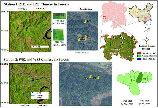
2.1. Study Sites
2.2. Field Data
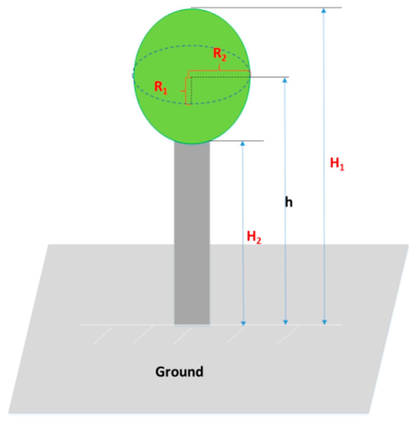
2.2.1. Canopy Structural Parameter Measurements
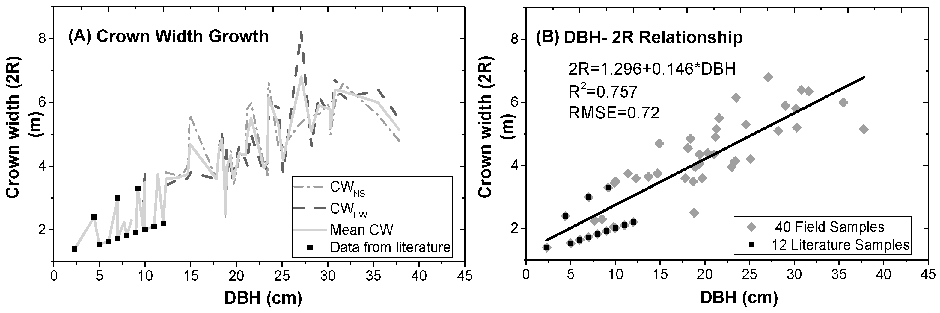
- Crown radius (R): R = (1.296 + 0.146 * DBH)/2, R2 = 0.76, RMSE = 0.72;
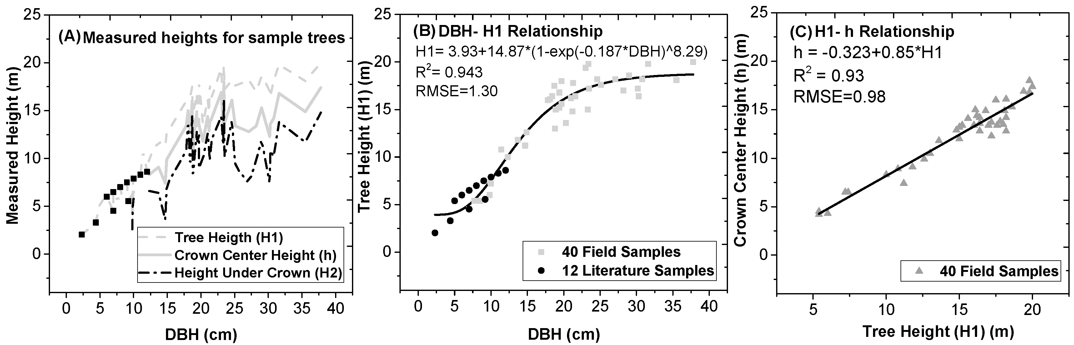
- Full tree height (H1): H1 = 3.928 + 14.866 * (1 − exp(−0.1865 * ), R2 = 0.94, RMSE = 1.30;
- Crown center height (h): h = −0.32 + 0.85 * H1, R2 = 0.93, RMSE = 0.98;
- Crown ellipticity (b/R), which was fixed at the mean value of the 40 field measurements: mean = 1.17, standard deviation (s.d.) = 0.46, since no significant relationship was found between b/R and DBH or H1.
2.2.2. LAI Measurements and Data Processing
2.2.3. Spectral Measurements: Leaf and Soil
2.3. Remote Sensing Observations
Landsat Observations
3. Methods
3.1. Theoretical Foundation
Geometrical Optical Radiative Transfer (GORT) Model
3.2. Contribution of Component LOPs to Canopy LOPs
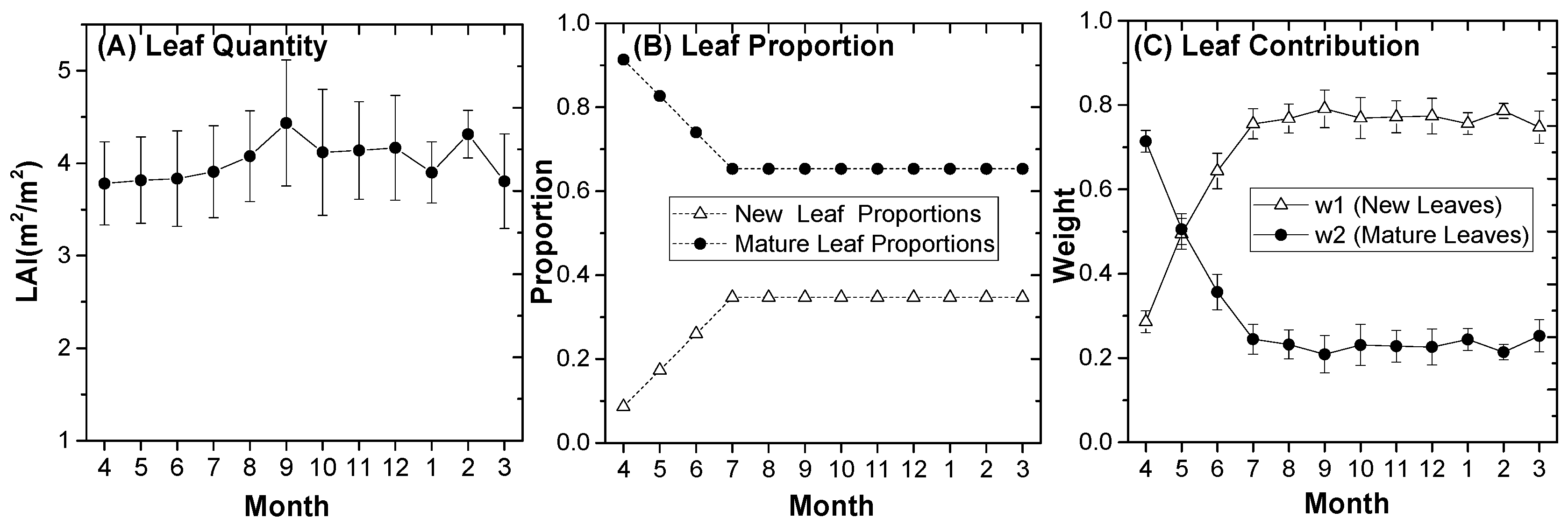
3.2.1. Leaf Area Proportion of New and Mature Leaves
3.2.2. Spatial Organization of New and Mature Leaves
3.3. LOPs at the Canopy Scale
3.3.1. Model Sensitivity Analysis
3.3.2. Model Inversion Strategy
3.3.3. Validation: Direct and Indirect Methods
4. Results
4.1. Sensitivity Analysis and Retrieval Results: GORT
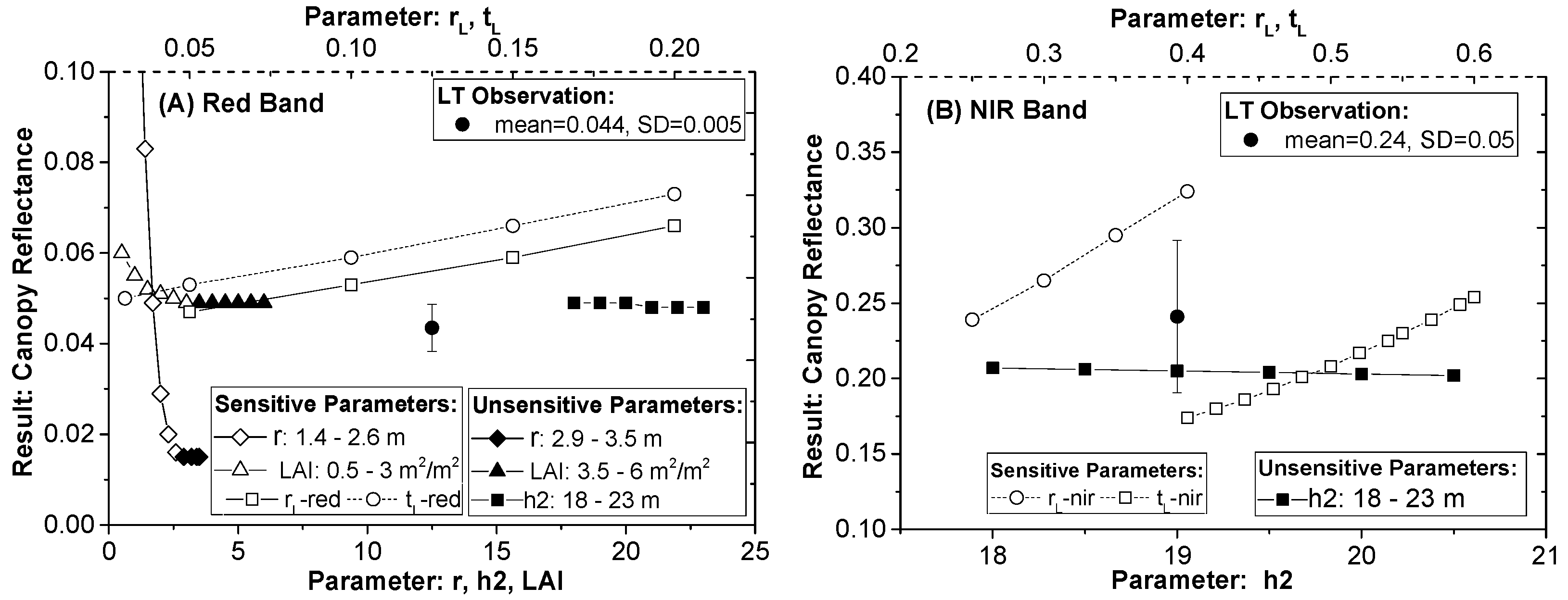
4.1.1. Total-Order and Single-Order Sensitivity Analysis Results
4.1.2. Prior Knowledge of Model Parameters
4.2. Optical Properties of Individual New and Mature Leaves
4.2.1. Leaves at Different Ages
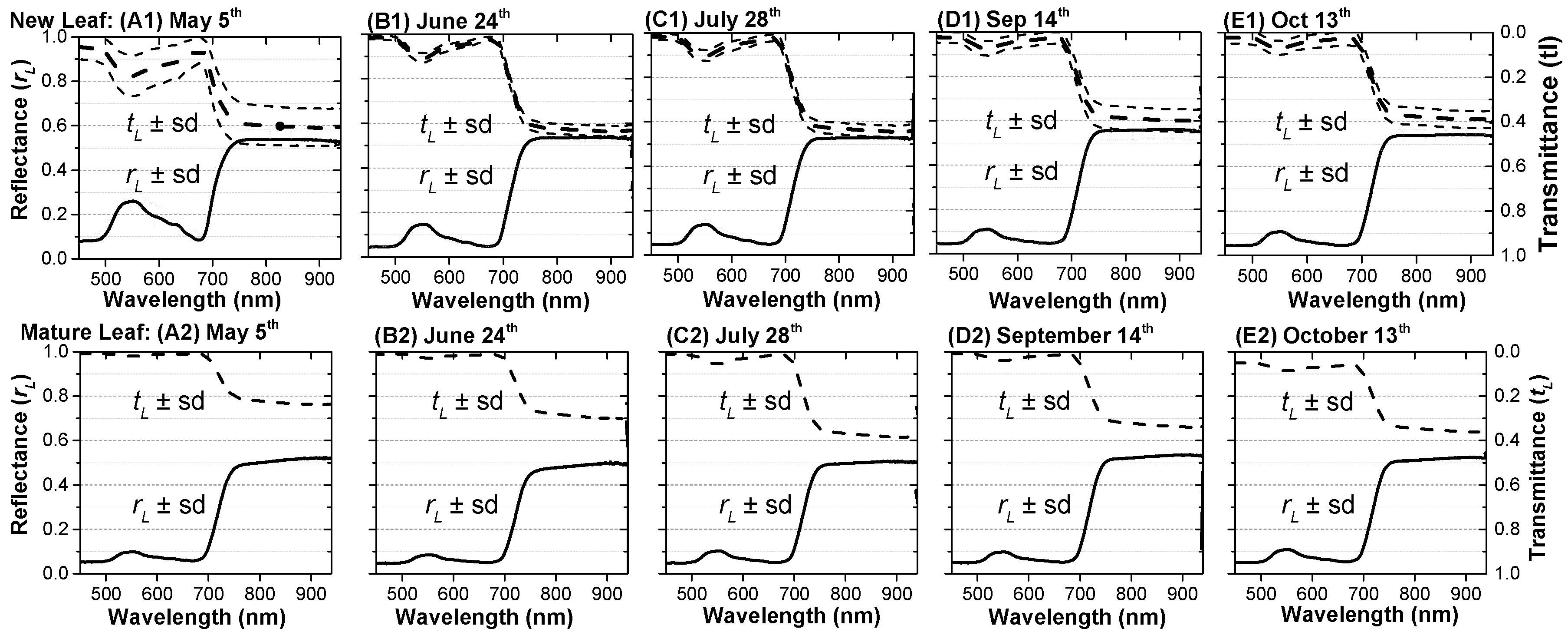
4.2.2. Leaves in Different Seasons
4.3. Leaf-Age Effects on Variability in Landsat-Viewed Canopy Reflectance
4.3.1. Leaf Optical Properties at the Canopy Scale
4.3.2. Seasonal Leaf Optical Properties
4.3.3. Leaf-Age Effects at Pixel Scale Based on Satellite Observations
- In the first circumstance, we ignore the leaf-age effects caused by aging mature leaves and growing new leaves, and only consider variations in LAI and sun geometry using field data. LOPs in the GORT model were fixed using the mean LOPs for mature leaves measured from May to September in 2017 (NIR band: REFmature = 0.51, TRAmature = 0.26 or 0.34; Red band: REFmature = 0.06, TRAmature = 0.01).
- Based on circumstance 1, we include variations in LOPs caused by aging mature leaves. For comparative purposes, we first added variations in mature leaves using data shown in Figure 10B1 to drive the GORT model.
- Based on circumstance 2, we further include variations in LOPs caused by production and expansion of new leaves. LOPs for the GORT model are shown in Figure 8B1. LOPs at the canopy scale retrieved at the ZH1 site are applied to the FZ1 site with different canopy structure parameters.
5. Discussion
5.1. Spectral Changes and Leaf Aging
5.2. Leaf-Aging Effects on Canopy Reflectance
5.3. Potential Implications for Photosynthesis
5.4. Implications of LOPs and Canopy Structure
6. Conclusions
- New leaf maturation is the main factor contributing to seasonality of canopy signals (NIR REF and EVI2), because of the distribution of these leaves in the top and outer canopy, as well as their increasing proportions with leaf growth. A small increase (0.05 unit) in new leaf NIR reflectance results in a significant increase in canopy NIR reflectance from spring to summer, while a decrease in new leaf NIR transmittance from August to October causes a decreasing trend in canopy NIR reflectance in autumn and winter.
- Mature leaf aging is another factor contributing to the seasonality of the canopy signals (NIR REF and EVI2) because of the significant proportion of mature leaves in the canopy. Mature leaf NIR transmittance is greater during the growing season than off the growing season. This difference in leaf TRA causes an increased difference in canopy reflectance between winter and summer.
Acknowledgments
Author Contributions
Conflicts of Interest
Appendix A
Appendix A.1. Data Description
Appendix A.2. Canopy Structural Parameter Measurements
Appendix A.3. Leaf Area Proportion and Distribution in Crown

| Leaf Age/Location | Bottom Crown | Central Crown | Upper Crown | Leaf Area ∑ (%) |
|---|---|---|---|---|
| 0 a | 1.16 | 1.41 | 3.24 | 5.8 (34.63%) |
| 1 a | 1.93 | 2.93 | 0.81 | 5.67 (33.85%) |
| 2 a | 1.80 | 1.59 | 0 | 3.39 (20.24%) |
| 3 a | 1.11 | 0.76 | 0 | 1.87 (11.64%) |
| Leaf Area ∑ (%) | 6.00 (35.8%) | 6.69 (40%) | 4.05 (24.2%) | 16.75 (100%) |
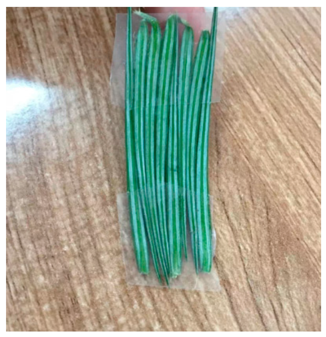
Appendix A.4. Leaf Sample for SVC Measurements
Appendix B
Appendix B.1. Data Description
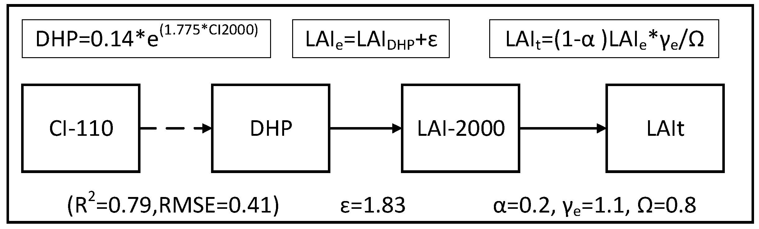
Appendix B.2. Long-Term LAIe Observations: DHP Methods
Appendix B.3. Converting LAIe to LAIt: LAI-2000 and TRAC Methods
Appendix B.4. Unifying LAI Measurements Using Different Methods
| Plot | ZH1 | FZ1 | ||||
|---|---|---|---|---|---|---|
| DHP (5 pts * 4 Dirs) | LAI-2000 (5 pts * 4 Dirs) | LAI-2000 (26 pts * 2 Repeat) | DHP (5 pts * 4 Dirs) | LAI-2000 (5 pts * 4 dirs) | LAI-2000 (61 pts * 3 Repeat) | |
| Maximum | 1.68 | 3.52 | 3.36 | 1.56 | 3.85 | 3.3 |
| Minimum | 1.37 | 2.9 | 3.19 | 1.05 | 2.87 | 3.18 |
| Mean | 1.533 | 3.186 | 3.275 | 1.282 | 3.248 | 3.243 |
| SD | 0.12 | 0.23 | 0.12 | 0.2 | 0.39 | 0.06 |
| System bias () * | _ | 1.653 | 1.724 | _ | 1.966 | 1.962 |
References
- Waring, R.H.; Schlesinger, W.H. Forest Ecosystems: Concepts and Management; Academic Press: Orlando, FL, USA, 1985; p. 75. [Google Scholar]
- Dixon, R.K.; Brown, S.; Houghton, R.E.A.; Solomon, A.; Trexler, M.; Wisniewski, J. Carbon pools and flux of global forest ecosystems. Science (Washington) 1994, 263, 185–189. [Google Scholar] [CrossRef] [PubMed]
- Schimel, D.; Stephens, B.B.; Fisher, J.B. Effect of increasing CO2 on the terrestrial carbon cycle. Proc. Natl. Acad. Sci. USA 2015, 112, 436–441. [Google Scholar] [CrossRef] [PubMed]
- Pan, Y.; Birdsey, R.A.; Fang, J.; Houghton, R.; Kauppi, P.E.; Kurz, W.A.; Phillips, O.L.; Shvidenko, A.; Lewis, S.L.; Canadell, J.G. A large and persistent carbon sink in the world’s forests. Science 2014, 333, 988–993. [Google Scholar] [CrossRef] [PubMed]
- Reich, P.B. Biogeochemistry: Taking stock of forest carbon. Nat. Clim. Chang. 2016, 1, 346–347. [Google Scholar] [CrossRef]
- Guyot, G.; Guyon, D.; Riom, J. Factors affecting the spectral response of forest canopies: A review. Geocarto Int. 1989, 4, 3–18. [Google Scholar] [CrossRef]
- Vermote, E.F.; Tanré, D.; Deuze, J.L.; Herman, M.; Morcette, J.-J. Second simulation of the satellite signal in the solar spectrum, 6s: An overview. IEEE Trans. Geosci. Remote Sens. 1997, 35, 675–686. [Google Scholar] [CrossRef]
- Samanta, A.; Ganguly, S.; Vermote, E.; Nemani, R.R.; Myneni, R.B. Why is remote sensing of Amazon forest greenness so challenging? Earth Interact. 2012, 16, 1–14. [Google Scholar] [CrossRef]
- Xiao, X.; Braswell, B.; Zhang, Q.; Boles, S.; Frolking, S.; Moore, B. Sensitivity of vegetation indices to atmospheric aerosols: Continental-scale observations in northern asia. Remote Sens. Environ. 2003, 84, 385–392. [Google Scholar] [CrossRef]
- Galvão, L.S.; dos Santos, J.R.; Roberts, D.A.; Breunig, F.M.; Toomey, M.; de Moura, Y.M. On intra-annual evi variability in the dry season of tropical forest: A case study with MODIS and hyperspectral data. Remote Sens. Environ. 2011, 115, 2350–2359. [Google Scholar] [CrossRef]
- Maeda, E.E.; Heiskanen, J.; Aragão, L.E.; Rinne, J. Can MODIS evi monitor ecosystem productivity in the Amazon rainforest? Geophys. Res. Lett. 2014, 41, 7176–7183. [Google Scholar] [CrossRef]
- Maeda, E.E.; Galvão, L.S. Sun-sensor geometry effects on vegetation index anomalies in the Amazon rainforest. GISci. Remote Sens. 2015, 52, 332–343. [Google Scholar] [CrossRef]
- Bi, J.; Knyazikhin, Y.; Choi, S.; Park, T.; Barichivich, J.; Ciais, P.; Fu, R.; Ganguly, S.; Hall, F.; Hilker, T. Sunlight mediated seasonality in canopy structure and photosynthetic activity of Amazonian rainforests. Environ. Res. Lett. 2015, 10, 064014. [Google Scholar] [CrossRef]
- Moura, Y.M.; Galvão, L.S.; dos Santos, J.R.; Roberts, D.A.; Breunig, F.M. Use of MISR/Terra data to study intra- and inter-annual EVI variations in the dry season of tropical forest. Remote Sens. Environ. 2012, 127, 260–270. [Google Scholar] [CrossRef]
- Lyapustin, A.I.; Wang, Y.; Laszlo, I.; Hilker, T.; Hall, F.G.; Sellers, P.J.; Tucker, C.J.; Korkin, S.V. Multi-angle implementation of atmospheric correction for MODIS (MAIAC): 3. Atmospheric correction. Remote Sens. Environ. 2012, 127, 385–393. [Google Scholar] [CrossRef]
- Jones, M.O.; Kimball, J.S.; Nemani, R.R. Asynchronous Amazon forest canopy phenology indicates adaptation to both water and light availability. Environ. Res. Lett. 2014, 9, 124021. [Google Scholar] [CrossRef]
- Goward, S.N.; Huemmrich, K.F. Vegetation canopy par absorptance and the normalized difference vegetation index: An assessment using the sail model. Remote Sens. Environ. 1992, 39, 119–140. [Google Scholar] [CrossRef]
- Ollinger, S.V. Sources of variability in canopy reflectance and the convergent properties of plants. New Phytol. 2011, 189, 375–394. [Google Scholar] [CrossRef] [PubMed]
- Asner, G.P. Biophysical and biochemical sources of variability in canopy reflectance. Remote Sens. Environ. 1998, 64, 234–253. [Google Scholar] [CrossRef]
- Jacquemoud, S.; Verhoef, W.; Baret, F.; Bacour, C.; Zarco-Tejada, P.J.; Asner, G.P.; François, C.; Ustin, S.L. Prospect+ sail models: A review of use for vegetation characterization. Remote Sens. Environ. 2009, 113, S56–S66. [Google Scholar] [CrossRef]
- Eriksson, H.M.; Eklundh, L.; Kuusk, A.; Nilson, T. Impact of understory vegetation on forest canopy reflectance and remotely sensed lai estimates. Remote Sens. Environ. 2006, 103, 408–418. [Google Scholar] [CrossRef]
- Jordan, C.F. Derivation of leaf-area index from quality of light on the forest floor. Ecology 1969, 50, 663–666. [Google Scholar] [CrossRef]
- Samanta, A.; Knyazikhin, Y.; Xu, L.; Dickinson, R.E.; Fu, R.; Costa, M.H.; Saatchi, S.S.; Nemani, R.R.; Myneni, R.B. Seasonal changes in leaf area of Amazon forests from leaf flushing and abscission. J. Geophys. Res. Biogeosci. 2012, 117. [Google Scholar] [CrossRef]
- Asner, G.P.; Alencar, A. Drought impacts on the Amazon forest: The remote sensing perspective. New Phytol. 2010, 187, 569–578. [Google Scholar] [CrossRef] [PubMed]
- Monteith, J.L.; Ross, J. The Radiation Regime and Architecture of Plant Stands; Springer: Dordrecht, The Netherlands, 1981; p. 344. [Google Scholar]
- Asner, G.P.; Wessman, C.A.; Schimel, D.S.; Archer, S. Variability in leaf and litter optical properties: Implications for BRDF model inversions using AVHRR, MODIS, and MISR. Remote Sens. Environ. 1998, 63, 243–257. [Google Scholar] [CrossRef]
- Doughty, C.E.; Goulden, M.L. Seasonal patterns of tropical forest leaf area index and CO2 exchange. J. Geophys. Res. Biogeosci. 2008, 113. [Google Scholar] [CrossRef]
- Wu, J.; Albert, L.P.; Lopes, A.P.; Restrepo-Coupe, N.; Hayek, M.; Wiedemann, K.T.; Guan, K.; Stark, S.C.; Christoffersen, B.; Prohaska, N. Leaf development and demography explain photosynthetic seasonality in Amazon evergreen forests. Science 2016, 351, 972–976. [Google Scholar] [CrossRef] [PubMed]
- Horler, D.; Ahern, F. Forestry information content of thematic mapper data. Int. J. Remote Sens. 1986, 7, 405–428. [Google Scholar] [CrossRef]
- Cohen, W.B.; Spies, T.A.; Fiorella, M. Estimating the age and structure of forests in a multi-ownership landscape of western Oregon, USA. Int. J. Remote Sens. 1995, 16, 721–746. [Google Scholar] [CrossRef]
- Jakubauskas, M.E. Thematic Mapper characterization of lodgepole pine seral stages in Yellowstone National Park, USA. Remote Sens. Environ. 1996, 56, 118–132. [Google Scholar] [CrossRef]
- Song, C.; Schroeder, T.A.; Cohen, W.B. Predicting temperate conifer forest successional stage distributions with multitemporal landsat thematic mapper imagery. Remote Sens. Environ. 2007, 106, 228–237. [Google Scholar] [CrossRef]
- Nilson, T.; Peterson, U. Age dependence of forest reflectance: Analysis of main driving factors. Remote Sens. Environ. 1994, 48, 319–331. [Google Scholar] [CrossRef]
- Eckenwalder, J.E. Conifers of the World: The Complete Reference; Timber Press: Portland, OR, USA, 2009. [Google Scholar]
- Chen, J.; Black, T.; Adams, R. Evaluation of hemispherical photography for determining plant area index and geometry of a forest stand. Agric. For. Meteorol. 1991, 56, 129–143. [Google Scholar] [CrossRef]
- Wagner, S. Calibration of grey values of hemispherical photographs for image analysis. Agric. For. Meteorol. 1998, 90, 103–117. [Google Scholar] [CrossRef]
- Englund, S.R.; O’brien, J.J.; Clark, D.B. Evaluation of digital and film hemispherical photography and spherical densiometry for measuring forest light environments. Can. J. For. Res. 2000, 30, 1999–2005. [Google Scholar] [CrossRef]
- Song, G.-Z.M.; Doley, D.; Yates, D.; Chao, K.-J.; Hsieh, C.-F. Improving accuracy of canopy hemispherical photography by a constant threshold value derived from an unobscured overcast sky. Can. J. For. Res. 2013, 44, 17–27. [Google Scholar] [CrossRef]
- Liu, Z.; Jin, G.; Chen, J.M.; Qi, Y. Evaluating optical measurements of leaf area index against litter collection in a mixed broadleaved-Korean pine forest in China. Trees 2015, 29, 59–73. [Google Scholar] [CrossRef]
- Tarantola, S.; Becker, W. Simlab software for uncertainty and sensitivity analysis. In Handbook of Uncertainty Quantification; Ghanem, R., Higdon, D., Owhadi, H., Eds.; Springer: Cham, Switzerland, 2016; pp. 1–21. [Google Scholar]
- Li, X.; Strahler, A.H.; Woodcock, C.E. Hybrid geometric optical-radiative transfer approach for modeling albedo and directional reflectance of discontinuous canopies. IEEE Trans. Geosci. Remote Sens. 1995, 33, 466–480. [Google Scholar]
- Ni, W.; Li, X.; Woodcock, C.E.; Caetano, M.R.; Strahler, A.H. An analytical hybrid gort model for bidirectional reflectance over discontinuous plant canopies. IEEE Trans. Geosci. Remote Sens. 1999, 37, 987–999. [Google Scholar]
- Li, X.; Strahler, A.H. Geometric-optical modeling of a conifer forest canopy. IEEE Trans. Geosci. Remote Sens. 1985, 23, 705–721. [Google Scholar] [CrossRef]
- Li, X.; Strahler, A.H. Geometric-optical bidirectional reflectance modeling of a conifer forest canopy. IEEE Trans. Geosci. Remote Sens. 1986, 24, 906–919. [Google Scholar] [CrossRef]
- Li, X.; Strahler, A.H. Geometric-optical bidirectional reflectance modeling of the discrete crown vegetation canopy: Effect of crown shape and mutual shadowing. IEEE Trans. Geosci. Remote Sens. 1992, 30, 276–292. [Google Scholar] [CrossRef]
- Serra, J. The boolean model and random sets. Comput. Graph. Image Process. 1980, 12, 99–126. [Google Scholar] [CrossRef]
- Li, X.; Strahler, A.H. Modeling the gap probability of a discontinuous vegetation canopy. IEEE Trans. Geosci. Remote Sens. 1988, 26, 161–170. [Google Scholar] [CrossRef]
- Ni, W.; Li, X.; Woodcock, C.E.; Roujean, J.-L.; Davis, R.E. Transmission of solar radiation in boreal conifer forests: Measurements and models. J. Geophys. Res. All Ser. 1997, 103, 29555–29566. [Google Scholar] [CrossRef]
- Song, C.; Woodcock, C.E.; Li, X. The spectral/temporal manifestation of forest succession in optical imagery: The potential of multitemporal imagery. Remote Sens. Environ. 2002, 82, 285–302. [Google Scholar] [CrossRef]
- Zhongkun, X.U.; Qingqian, X.U.; Rong, J. The characters of leaf area and net photosynthesis efficiency of needle at different parts and in different leaf age of Cunninghamia lanceolata. Hunan For. Sci. Technol. 2008, 41, 1–4. [Google Scholar]
- Saltelli, A.; Bolado, R. An alternative way to compute fourier amplitude sensitivity test (FAST). Comput. Stat. Data Anal. 1998, 26, 445–460. [Google Scholar] [CrossRef]
- Shi, H.; Xiao, Z.; Liang, S.; Zhang, X. Consistent estimation of multiple parameters from MODIS top of atmosphere reflectance data using a coupled soil-canopy-atmosphere radiative transfer model. Remote Sens. Environ. 2016, 184, 40–57. [Google Scholar] [CrossRef]
- Saltelli, A.; Annoni, P.; Azzini, I.; Campolongo, F.; Ratto, M.; Tarantola, S. Variance based sensitivity analysis of model output. Design and estimator for the total sensitivity index. Comput. Phys. Commun. 2010, 181, 259–270. [Google Scholar] [CrossRef]
- Saltelli, A.; Tarantola, S.; Chan, K.P.-S. A quantitative model-independent method for global sensitivity analysis of model output. Technometrics 1999, 41, 39–56. [Google Scholar] [CrossRef]
- Saltelli, A.; Tarantola, S.; Campolongo, F.; Ratto, M. Sensitivity analysis in practice. J. Am. Stat. Assoc. 2004, 101, 398–399. [Google Scholar]
- Li, X.; Gao, F.; Wang, J.; Zhu, Q. Uncertainty and sensitivity matrix of parameters in inversion of physical BRDF model. J. Remote Sens. 1997, 1, 161–172. [Google Scholar]
- Tarantola, A. Inverse Problem Theory and Methods for Model Parameter Estimation; Society for Industrial and Applied Mathematics (SIAM): Philadelphia, PA, USA, 2005. [Google Scholar]
- Nocedal, J.; Wright, S.J. Sequential Quadratic Programming; Springer: New York, NY, USA, 2006. [Google Scholar]
- Lin, Z.F.; Ehleringer, J. Changes in spectral properties of leaves as related to chlorophyll content and age of papaya. Photosynthetica 1982, 16, 520–525. [Google Scholar]
- Roberts, D.A.; Nelson, B.W.; Adams, J.B.; Palmer, F. Spectral changes with leaf aging in Amazon caatinga. Trees 1998, 12, 315–325. [Google Scholar] [CrossRef]
- Rock, B.N.; Williams, D.L.; Moss, D.M.; Lauten, G.N.; Kim, M. High-spectral resolution field and laboratory optical reflectance measurements of red spruce and eastern hemlock needles and branches. Remote Sens. Environ. 1994, 47, 176–189. [Google Scholar] [CrossRef]
- Gausman, H.W.; Allen, W.A.; Cardenas, R.; Richardson, A.J. Reflectance discrimination of cotton and corn at four growth stages. Agron. J. 1973, 65, 194–198. [Google Scholar] [CrossRef]
- Chavanabryant, C.; Malhi, Y.; Wu, J.; Asner, G.P.; Anastasiou, A.; Enquist, B.J.; Cosio Caravasi, E.G.; Doughty, C.E.; Saleska, S.R.; Martin, R.E. Leaf aging of Amazonian canopy trees as revealed by spectral and physiochemical measurements. New Phytol. 2017, 214, 1049–1063. [Google Scholar] [CrossRef] [PubMed]
- Samanta, A.; Ganguly, S.; Myneni, R.B. MODIS enhanced vegetation index data do not show greening of Amazon forests during the 2005 drought. New Phytol. 2011, 189, 11–15. [Google Scholar] [CrossRef] [PubMed]
- Samanta, A.; Costa, M.H.; Nunes, E.L.; Vieira, S.A.; Xu, L.; Myneni, R.B. Comment on drought-induced reduction in global terrestrial net primary production from 2000 through 2009. Science 2011, 333, 1093. [Google Scholar] [CrossRef] [PubMed]
- Xu, L.; Samanta, A.; Costa, M.H.; Ganguly, S.; Nemani, R.R.; Myneni, R.B. Widespread decline in greenness of Amazonian vegetation due to the 2010 drought. Geophys. Res. Lett. 2011, 38, 490–500. [Google Scholar] [CrossRef]
- Toomey, M.; Roberts, D.; Nelson, B. The influence of epiphylls on remote sensing of humid forests. Remote Sens. Environ. 2009, 113, 1787–1798. [Google Scholar] [CrossRef]
- Xiaoquan, Z.; Deying, X. Seasonal changes and daily courses of photosynthetic characteristics of 18-year-old chinese fir shoots in relation to shoot ages and positions within tree crown. Sci. Silvae Sin. 2000, 36, 19–26. [Google Scholar]
- Wu, J.; Serbin, S.P.; Xu, X.; Albert, L.P.; Chen, M.; Meng, R.; Saleska, S.R.; Rogers, A. The phenology of leaf quality and its within-canopy variation are essential for accurate modeling of photosynthesis in tropical evergreen forests. Glob. Chang. Biol. 2017, 23, 4814–4827. [Google Scholar] [CrossRef] [PubMed]
- Frazer, G.W.; Fournier, R.A.; Trofymow, J.A.; Hall, R.J. A comparison of digital and film fisheye photography for analysis of forest canopy structure and gap light transmission. Agric. For. Meteorol. 2001, 109, 249–263. [Google Scholar] [CrossRef]
- Zhang, Y.; Chen, J.M.; Miller, J.R. Determining digital hemispherical photograph exposure for leaf area index estimation. Agric. For. Meteorol. 2005, 133, 166–181. [Google Scholar] [CrossRef]


| Symbols | Parameters | Source |
|---|---|---|
| Canopy Structure Parameters | ||
| h1 | lower boundary of canopy center height | O 1 and CERN 2 |
| h2 | upper boundary of canopy center height | O and CERN |
| R | horizon mean crown radius | O and CERN |
| b/R | crown spheroid ellipticity | 1.17 (O) |
| tree stem density (trees/ha) | CERN | |
| FAVD | foliage area volume density (m2/m3) | O and CERN |
| k | leaf angle distribution factor | 0.5 (random) |
| Component Spectral Parameters | ||
| leaf reflectance | O | |
| leaf transmittance | O | |
| rG | soil/background reflectance | O |
| Sun-Sensor Geometry | ||
| SZN | sun zenith angle (°) | Time, Lon, Lat 3 |
| VZN | view zenith angle (°) | 0 |
| VAZ | view azimuth angle (°) | 0 |
| Parameter | Results | Prior Knowledge * (s.d.) | Lower Limit | Upper Limit |
|---|---|---|---|---|
| - | - | 0.07 | 5.27 | |
| - | - | 1.49 | 13.5 | |
| - | - | 2.48 | 22.5 | |
| stem density () | - | - | 0.1035 | 0.252 |
| crown radius () 1 | 1.7 | 1.5 | 0.92 | 2.57 |
| -red | 0.07(0.02) | 0.05 | 0.12 | |
| -red | 0.04(0.03) | 0.02 | 0.1 | |
| -red | - | - | 0.3 | 0.4 |
| -nir | 0.52(0.02) | 0.35 | 0.6 | |
| -nir 1 | 0.36(0.05) | 0.25 | 0.4 | |
| -nir 1 | - | - | 0.35 | 0.45 |
© 2018 by the authors. Licensee MDPI, Basel, Switzerland. This article is an open access article distributed under the terms and conditions of the Creative Commons Attribution (CC BY) license (http://creativecommons.org/licenses/by/4.0/).
Share and Cite
Wu, Q.; Song, C.; Song, J.; Wang, J.; Chen, S.; Yu, B. Impacts of Leaf Age on Canopy Spectral Signature Variation in Evergreen Chinese Fir Forests. Remote Sens. 2018, 10, 262. https://doi.org/10.3390/rs10020262
Wu Q, Song C, Song J, Wang J, Chen S, Yu B. Impacts of Leaf Age on Canopy Spectral Signature Variation in Evergreen Chinese Fir Forests. Remote Sensing. 2018; 10(2):262. https://doi.org/10.3390/rs10020262
Chicago/Turabian StyleWu, Qiaoli, Conghe Song, Jinling Song, Jindi Wang, Shaoyuan Chen, and Bo Yu. 2018. "Impacts of Leaf Age on Canopy Spectral Signature Variation in Evergreen Chinese Fir Forests" Remote Sensing 10, no. 2: 262. https://doi.org/10.3390/rs10020262