Incorporation of Stem Water Content into Vegetation Optical Depth for Crops and Woodlands
by
E. Raymond Hunt
1,*, 
Li Li
2,
Jennifer M. Friedman
1,
Peter W. Gaiser
2,
Elizabeth Twarog
2 and
Michael H. Cosh
1 
1
Hydrology and Remote Sensing Laboratory, USDA Agricultural Research Service, Beltsville Agricultural Research Center, Beltsville, MD 20705, USA
2
Naval Research Laboratory, Washington, DC 20375, USA
*
Author to whom correspondence should be addressed.
Remote Sens. 2018, 10(2), 273; https://doi.org/10.3390/rs10020273
Submission received: 13 December 2017
/
Revised: 5 February 2018
/
Accepted: 8 February 2018
/
Published: 10 February 2018
(This article belongs to the Section Remote Sensing in Agriculture and Vegetation)
Abstract
:Estimation of vegetation water content (VWC) by optical remote sensing improves soil moisture retrievals from passive microwave radiometry. For a variety of vegetation types, the largest unknown for predicting VWC is stem water content, which is assumed to be allometrically related to the water content of the plant canopy. For maize and soybean, measured stem water contents were highly correlated to canopy water contents, so VWC was calculated directly from the normalized difference infrared index (NDII), which contrasts scattering at near-infrared wavelengths with absorption of shortwave infrared wavelengths by liquid water. Woodland tree height is linearly related to woody stem volume, and hence to stem water content. We hypothesized that tree height is positively correlated with canopy water content, and thus with NDII. Airborne color-infrared imagery was acquired at two study areas in a mixed agricultural and woodland landscape, and photogrammetric structure-from-motion point clouds were derived to estimate tree heights. However, estimated tree heights were only weakly correlated with measured data acquired for validation. NDII was calculated from Landsat 8 Operational Line Imager (30-m pixel) and WorldView-3 (7.5 m pixel); but contrary to the hypothesis, NDII was not correlated with woodland tree height. Lastly, the interaction of woodland and crops stem water contents on total VWC in a mixed landscape were simulated for 2 days, one in the early summer and one in the late summer. VWC for the region varied from 2.5 to 3.0 kg m−2, which was just under a threshold for accuracy for soil moisture retrievals using Coriolis WindSat. Woodland tree height should be included as an ancillary data set along with land cover classification for soil moisture retrieval algorithms.
1. Introduction
Retrieval of soil moisture content from passive microwave brightness temperatures is based on the zero-order tau-omega (τfp − ωfp) model, where: τfp is the vegetation optical depth at frequency f and polarization p, and ωfp is the single scattering albedo at frequency f and polarization p [1,2,3]. Vegetation optical depth occurs in two of the three terms of the tau-omega model, and it is estimated by the product of an attenuation factor (denoted by b) and vegetation water content (VWC, kg m−2) [3,4]. The attenuation factor depends on frequency, polarization and canopy structure [3,4]. Initial work on soil moisture retrievals using passive microwave radiometers was performed in areas with short vegetation cover, in which VWC was easily measured and had small effects on estimated soil moisture [5,6]. For these cover types, the foliar leaf area index (LAI, m2 m−2), the fractional vegetation cover, and canopy water content (CWC, kg m−2) are excellent predictors of VWC.
There are several spectral vegetation indices used to estimate vegetation optical depth [7,8,9,10,11,12,13]. Spectral vegetation indices contrast multiple scattering of near-infrared (NIR) radiation by the foliage with either absorption of red radiation by chlorophyll or absorption of shortwave-infrared radiation (SWIR) by liquid water [14]. CWC is defined as the product of LAI and average leaf water content; thus, CWC may be estimated with spectral NIR-Red vegetation indices that are correlated with LAI, such as the normalized difference vegetation index (NDVI) [15]. Since leaf water content varies by plant species or plant functional type, relationships between NIR-Red indices and VWC are highly empirical [16]. On the other hand, NIR-SWIR spectral indices, such as the normalized difference infrared index (NDII) [17] and the normalized difference water index (NDWI) [18], are sensitive to both LAI and leaf water content. Thus, estimation of VWC using NIR-SWIR indices is less empirical than NIR-Red indices [8,19]. For most vegetation types, NDII is linearly related with CWC up to about 0.8 kg m−2 [19,20,21].
Stem water contents (SWC, kg m−2) contribute to vegetation optical depths for forests, woodlands, and tall crops [8,10,11,22,23,24]. Both data and theory indicate that the dry masses of leaves and stems are allometrically related for structural support and hydraulic transport [25,26,27,28,29,30]. If water contents of leaves and stems are proportional to dry mass, then SWC will be allometrically related to CWC, subsequently leading to correlations between SWC and spectral indices. Different vegetation types have different allometric relationships between CWC and SWC, which lead to different relationships between spectral indices and VWC. The passive microwave retrieval algorithm for the Soil Moisture Active Passive (SMAP) mission makes the allometric relationships between SWC and CWC explicit in terms of a stem factor for different vegetation land cover classes [31,32]. The overall goal of our research was to improve application of spectral vegetation indices for estimating vegetation optical depth, by examining two methods of estimating SWC from CWC.
Our first objective is to compare SWC and CWC for two crops, maize (Zea mays L.) and soybean [Glycine max (L.) Merr.], to determine if measurements on single plants may be used in place of plot-based measurements. Most studies on VWC make plot-based measurements acquired concurrently with remotely sensed data. In addition to random statistical variation, differences in weather, plant density, and developmental growth stage may cause additional variation in relationships between VWC and spectral indices, and that variation may bias soil moisture retrievals. Hence, large numbers of plots need to be sampled to derive robust equations for agricultural regions. Since NDII was linear for the range of CWC, the effects of non-random variation were included in remotely sensed CWC. A fast method of obtaining the allometric relationships between SWC from CWC would then allow vegetation optical depth to be determined with less empiricism than estimating VWC from NDVI.
For woodland and forest land cover types, SWC may be many times greater than CWC; therefore, small random errors or biases in allometric relationships between leaves and stems will have large impacts on estimated vegetation optical depth and the accuracy of retrieved soil moisture content. Deciduous woodlands and forests are perennial cover types, so there will be little change in SWC over a year compared to phenological changes in CWC. Furthermore, it is not practical to measure SWC and CWC for mature trees. For cylinders, cones, and similar geometric solids, volume is proportional to height. Thus, stem volume may be estimated from tree height using either lidar or photogrammetric methods [33,34,35]. If SWC is allometrically related to CWC, we hypothesize that tree height will be positively correlated with the annual maximum CWC. Our second objective is to test this hypothesis with tree heights derived from airborne imagery and CWC estimated from NIR-SWIR spectral indices.
The accuracy of soil moisture retrievals using the tau-omega (τfp − ωfp) model varies with microwave frequency; radiometers that use higher frequencies for retrievals require more accuracy for VWC [3]. WindSat is a multi-frequency dual-polarization passive microwave radiometer developed by the Naval Research Laboratory, which was launched on the US Department of Defense Coriolis satellite on 6 January 2003 [36]. The primary objective of the WindSat mission was to test the ability of polarimetric microwave radiometers to determine both the speed and direction of ocean-surface winds. A secondary objective for WindSat was the simultaneous retrieval of soil moisture content, VWC and land surface temperature from vertically and horizontally polarized brightness temperatures at frequencies of 10 GHz, 18.7 GHz and 37 GHz [37]. The 6-GHz channels on WindSat are not used for soil moisture retrievals because of extensive radio frequency interference [38]. Crops such as maize have large increases of SWC over the growing season, but these changes are small compared to woodland SWC. Our third objective is to simulate the potential effectiveness of both SWC remote sensing methods over a large mixed area of cropland and woodlands in relation to the expected errors for soil moisture retrievals.
2. Methods
2.1. Allometric Model for Vegetation Water Content
Allometric growth is the change in a species geometric form (length, area, volume) with an increase in size to maintain structural support, mass transport or other physical requirements [25,26,27,28]. In general, growth of plant stems and leaf area are allometrically related, which serves as a theoretical basis for estimating stem dry matter or volume using an exponential function:
where: Mc and Ms are the mass in the canopy and stems, respectively, and α and β are the allometric coefficients (β equals 1 for a linear relationship). Supporting the general hypothesis, satellite sensors such as Landsat are used to estimate aboveground forest biomass from canopy reflectances [39,40,41], so there is some predictive relationship between remotely-sensed canopy variables and the stems hiding underneath. Water contents of stems and leaves are related to the dry matter contents per volume; therefore, SWC should be allometrically related to CWC. VWC is the sum of CWC and SWC.
Ms = α Mc β
Current methods for estimating VWC are to measure water contents per ground area along with spectral reflectances. However, acquiring sufficient plot data for robust predictions is time consuming, which provides an opportunity for water loss by evaporation to bias the relationships. Previous results suggested that the relationship between SWC and CWC is linear for crops [19], so VWC may be estimated directly from CWC:
where ξ (Greek letter xi for xylem) is a coefficient for the relationship between stem and leaf water contents, and (1 + ξ) is the slope of the SWC-CWC line. Effects of both plant density and LAI are included in CWC estimated remotely using NIR-SWIR vegetation indices.
VWC = (1 + ξ) CWC,
2.2. Study Areas and Field Measurements
At the USDA-ARS Beltsville Agricultural Research Center in Beltsville, Maryland (Figure 1), eight and six fields of maize and soybean, respectively, were selected for sampling. These fields had different planting dates ranging from late April to early July 2015. Different varieties of maize and soybean were planted to compensate for differences in growing season length. Maize and soybean fields planted earlier in the season experienced colder temperatures and higher precipitation during initial growth compared to fields planted later in the season. Effectively the crops germinated and grew under different weather conditions. Two plants from each field were collected weekly from early vegetative growth stages through the mid reproductive growth stages. Stems and leaves were weighed, dried at 65° C, and weighed again. Water contents were the difference between fresh and dry weight.
The other research location was the Choptank River Watershed on Maryland’s Eastern Shore of the Chesapeake Bay (Figure 1). This area was the site for the SMEXVEX08 experiment [42,43]. Land cover type and crop type for 2015 were obtained from the USDA National Agricultural Statistics Service’s Cropland Data Layer [44,45]. The land cover is about 30% maize, 30% soybean, and 33% woodland, with the remainder being housing developments, wetlands, pastures, and other crops. The woodlands are geographically associated with wetlands and streams, which prevented these areas from being cultivated in the recent past. USDA-NASS assessed producer and user accuracies were 93.8% and 84.8% for maize, respectively, and 87.5% and 79.9% for soybean, respectively [46]. In 2014, an independent accuracy assessment of the Cropland Data Layer in the Choptank River Watershed found the overall classification accuracy was 94% (unpublished data). Stations to monitor soil water content were established in cooperation with private landowners, University of Maryland Extension agents, and the United States Geological Survey.
Woodland stand height was determined from roadsides using a Nikon Inc. (Toyko, Japan) Forestry Pro Laser Rangefinder, which measured the distance to a tree, and the angle from the base to the top of the tree. The latitude and longitude for each stand was measured with a Garmin Inc. (Olathe, KS, USA) GPSmap 62st global positioning system.
2.3. Image Data
DigitalGlobe (Westminster, Colorado, USA) WorldView-3 (WV-3) visible/near-infrared (VNIR) and SWIR data were acquired 16 August 2015 in the two areas (A and B) in Figure 1. Images were geospatially registered by DigitalGlobe. All image processing was performed using the Harris Geospatial Solutions (Broomfield, CO, USA) Environment for Visualizing Images (ENVI) version 5.4. The WV-3 data were atmospherically corrected to land surface reflectances using the ENVI FLAASH package. The pixel sizes of WV-3’s VNIR and SWIR spectroradiometers are 1.2 and 7.5 m, respectively, the VNIR layers were resampled to the SWIR layers, so final pixel sizes were 7.5 m (Table 1).
Landsat 8 Operational Land Imager (L8-OLI) data were acquired on 17 August 2015 (WR2 path 15 and row 33), one day after the WV-3 acquisition. The L8-OLI data were atmospherically corrected to land surface reflectances using the ENVI FLAASH package.
There are many spectral indices based on NIR-SWIR reflectances suitable for estimation of foliar water content and CWC [21]. The normalized difference infrared index (NDII) [17] was calculated:
where: RNIR is the reflectance at near-infrared (NIR) wavelengths and RSWIR is the reflectance at SWIR wavelengths at about 1650 nm wavelength. For analysis of the WV-3 data, RNIR was the NIR-1 and RSWIR was SWIR band 3 (Table 1). For the L8-OLI analysis, RNIR was NIR band 5 and RSWIR was SWIR-1 band 6 (Table 1). The predictive ability of NDII for leaf and canopy water content was equal to or better than other indices [21].
NDII = (RNIR − RSWIR)/(RNIR + RSWIR),
Airborne digital color-infrared photographs were acquired over two areas to determine woodland height (Figure 1). A proprietary camera system was flown at 1700 m above ground level on 7 August 2014 by FalconScan LLC (Crofton, MD, USA). The front-to-back overlap of successive photographs was 75% and side-to-side overlap of adjacent flight lines was 50%. The center point (longitude, latitude, and elevation) for each photograph was calculated from global positioning system and inertial measurement unit data.
A recent method for estimating tree height uses photogrammetric “Structure from Motion” (SfM) point clouds [47,48,49] obtained from numerous overlapping aerial images. The 8-bit TIFF photographs were processed using Agisoft LLC (St. Petersburg, Russia) Photoscan Pro version 1.26 to generate SfM point clouds, from which digital surface elevation models and color-infrared orthomosaic images were generated. Without ground control points, there were curvature artifacts in the initial digital surface elevation models. To reduce the artifacts, 30 ground control points at ground level for each area were determined using GoogleEarth (Google Inc., Mountain View, CA, USA). The accuracy of these ground control points was not known, because location accuracy in GoogleEarth depends on several factors, such as the numbers and types of images (Google Inc. personal communication).
To test the geolocation accuracy of the airborne color-infrared orthomosaics, another 30 control points at ground level in each area were identified in both the orthomosaic images and WV-3 imagery. Root mean square errors (RMSE) between the airborne and WV-3 images were 5.6 m for box A and 10.8 m for box B (Figure 1).
Stand height profiles were determined from the digital surface elevation models at each location where tree heights were measured; each profile went from bare fields or roads, through the stand being measured. Relative stand heights (m) were the difference between the elevation at the 90th percentile on the profile elevation frequency distribution and the local elevation of the adjacent ground. The relative stand heights were compared to the measured tree heights in the two study areas.
2.4. Regional Simulations of VWC
Regional CWC and VWC were calculated from L8-OLI imagery (WR2 path 14 row 33) for the study areas and surrounding area on two dates, early summer (23 June 2015) and late summer (26 August 2015). Both images were atmospherically corrected with the ENVI FLAASH package. The USDA-NASS Cropland Data Layer for 2015 was used for land cover type [46]. Previous work with crops, grasslands, and deciduous woodlands [19,20] established that for the range of NDII found, the relationship between NDII and CWC was linear:
where the linear regression’s RMSE was 0.091 kg m−2 and the R2 was 0.847.
CWC = 0.230 + 1.18 NDII,
Maize and soybean VWC were calculated using Equation (2) from CWC and measured ξ (Figure 2). VWC of wheat, pasture and grass, and herbaceous wetlands were assumed to equal to CWC. The VWC for non-vegetated land cover was set to zero.
Nelson et al. [50] established an allometric relationship for calculating stem volume based on tree heights in Delaware, USA, which was next to the study area (Figure 1). We used Nelson et al.’s Equation (2) [50]:
where V is wood volume (m3 ha−1) and h is the average stand height in meters. Generally, water content of wood is about 0.4 m3 m−3 [51], so SWC was set to 0.4V. There is more variation in wood gravimetric water contents (kg water kg−1 wood) among species because there is a large variation in wood density [52]. Relative stand heights were estimated from profiles of the digital surface elevation models from bare ground through the center of each stand. Mean relative stand height was used to calculate SWC, which was then added to remotely sensed CWC to obtain woodland VWC (Figure 2).
V = 11.6h − 17,
The area covered by open water and wetlands is essential for soil moisture retrievals [53] but was not included to emphasize the contribution of woodland SWC and VWC. Image VWC was averaged over a circle of 25-km diameter (about 545,000 total pixels).
3. Results and Discussion
3.1. Crop Vegetation Water Content
There were strong linear relationships between leaf and stem water contents for maize and soybean (Figure 3). The coefficient ξ was 2.86 for maize and 1.71 for soybean. Crop CWC is important for estimating VWC, and hence vegetation optical depth, because it could be estimated directly from NDII. NDVI and NDII are highly correlated. NDVI accounts for differences in LAI and canopy structure, but the chlorophyll extinction coefficient is very large at red wavelengths, so NDVI saturates at lower LAI compared to NDII. Furthermore, estimating CWC from NDVI will require additional parameters such as the ratio of leaf water content to chlorophyll content and wood density.
3.2. Woodland Stand Height
The color-infrared orthomosaics for the two areas covered by the manned aircraft were derived from the individual aerial photographs are shown in Figure 4a and Figure 5a. The digital surface elevation models are shown in Figure 4b and Figure 5b. Wooded areas visible on the orthomosaics are clearly higher than the surrounding fields of crops and bare soil.
The elevation above sea level from GoogleEarth had an overall mean of about 20 m above sea level from the ground control point data. However, there were surface artifacts along the sides of the elevation model (Figure 4b and Figure 5b) because fewer photographs were available for the SfM algorithm. Woodland surface heights varied from 20 to 65 m above mean sea level. Correcting woodland surface heights using a profile from roads or bare ground resulted in a range from 1.9 to 30.7 m, with a mean of 15.8 m and a standard deviation of 7.0 m
Measured stand heights varied from 7 to 31 m with a mean of 18 m and a standard deviation of 5 m. Relative woodland stand heights were weakly correlated (Pearson r = 0.42) with the measured stand heights (Figure 6). Stratifying the stand data into various subsets (e.g., boxes A and B, deciduous and conifer) did not improve the agreement between relative and measured stand heights.
3.3. Spectral Indices and Stand Height
L8-OLI and WV-3 false color composites showed spectral differences (Figure 7 and Figure 8) even though both data sets were atmospherically corrected to ground surface reflectances. Calculation of NDII reduced the differences (Figure 9), but L8-OLI NDII was higher mostly because the NIR reflectances were higher. Using either L8-OLI or WV-3 imagery, NDII did not have a significant correlation with measured stand height (Figure 9a) or relative height (Figure 9b) estimated from the digital surface model. Therefore, the hypothesis that allometric relationships between CWC and SWC could be used to estimate VWC from NDII was rejected. However, this result was not conclusive because of the weak correlation between relative stand heights from the point cloud and measured stand heights from a laser rangefinder (Figure 6). Furthermore, there were no correlations between NDII and the measured stand heights and between NDVI of the color-infrared orthomosaics and relative stand heights. In general, heights from SfM and lidar point clouds are comparable, but each method has its strengths and weaknesses [54,55]. Several ad-hoc hypotheses may be proposed to explain the reason that NDII was not correlated with stand height based on analogies with lidar remote sensing [56,57]. The simplest explanations are either the null hypothesis was correct at the stand scale, or the measurement errors were too large to reject the null hypothesis.
Why did the crops have a strong allometric relationship but the woodlands didn’t? There are two possibilities, the first is that trees are perennial and accumulate woody biomass, which is not living at functional maturity. Crops like maize and soybean are annuals, for which most of the liquid water in stems is in living parenchyma tissues. Second, except for a few coniferous tree plantations in the study area, each stand contained: (a) many different tree species; (b) a variable number of trees per stand; and (c) a range of stem diameters, heights and age classes. Variation in allometric relationships among tree species may have been important [58], whereas we assumed there would be one general relationship based on the deciduous broadleaf tree functional type.
4. Importance of SWC for Soil Moisture Retrievals
Remotely sensed soil moisture is an important data source for agricultural drought monitoring [3]. In regions with a mixture of woodlands and croplands, changes of crop SWC over the growing season are small compared to woodland SWC, so accurate estimations of woodland SWC are necessary for assessing drought. Therefore, simulations were conducted using L8-OLI and land cover data over the study area to compare the importance of an independent estimates of SWC for calculation of VWC (Figure 2).
4.1. Inversion of WindSat Brightness Temperatures
The algorithm for Coriolis WindSat developed by Li et al. [37] retrieves three parameters (surface temperature, soil moisture content, and VWC) from six brightness temperatures (horizontal and vertical polarizations at 10.7, 18.7, and 37.0 GHz) (Figure 10). Sensitivity of soil moisture retrieval to VWC was estimated by varying the three parameters and calculating the six brightness temperatures using the τfp - ωfp model. Then, random noise was added to the brightness temperatures, where the random noise had a Gaussian distribution with zero mean and constant variance. The three parameters were retrieved using a maximum likelihood inversion method [37]. The difference between the input and output soil moisture, divided by the input soil moisture, was the relative error in soil moisture retrieval. This procedure was repeated about 10,000 times to determine the error of soil moisture retrieval at a given VWC (Figure 10).
With greater VWC, simulated errors in retrieved soil moisture content increase exponentially (Figure 10). At a VWC of about 4 kg m−2, soil moisture retrievals are expected to have a 10% error. The sensitivity of WindSat to soil moisture content is less than the Soil Moisture Active Passive (SMAP) and the Soil Moisture Ocean Salinity (SMOS) radiometers, because SMAP and SMOS microwave channels are at a frequency of 1.4 GHz [3]. To compensate for WindSat’s lower sensitivity, it is necessary to obtain the highest possible accuracies for vegetation optical depth from independent remote sensing sources. Then, only two parameters would need to be retrieved from the six brightness temperatures, potentially increasing retrieval accuracy.
4.2. Limits of Woodland Cover for WindSat Retrievals
From Equation 5, a stand with a mean relative tree height of 16 m would be expected to have a stem water content of 6.7 kg m−2 (Figure 11). Since the study area was about one-third woodlands, area weighted SWC would be about 2.2 kg m−2. With 100% tree cover and tree heights of only 10 m, the predicted SWC would equal 4 kg m−2, the threshold for soil moisture retrievals from WindSat (Figure 11). Regional SWC, and thus VWC, depends on the product of woodland cover and woodland height. Therefore, soil moisture retrievals from WindSat for areas with mixtures of vegetation types would be more accurate if ancillary tree height data were included with NDII and a land cover classification.
4.3. Changes of SWC and VWC over a Growing Season
Different vegetation types are usually not distributed randomly across mixed regions such as the Eastern Shore of the Chesapeake Bay (Figure 12). Over a growing season, maize has the largest increase of SWC, but the change is small compared to constant woodland SWC. The VWC of maize was low in early summer, so the VWC averaged over the Choptank River watershed was about 2.5 kg m−2 (Figure 13a). In late summer, maize VWC was at its maximum, increasing the watershed average VWC to about 3.0 kg m−2 (Figure 13b). Because VWC was close to the selected threshold of 4.0 kg m−2, using VWC as an input, rather than including it in the retrieval, would be expected to increase the accuracy for retrieved soil moisture contents.
5. Conclusions
Stem water contents are the largest unknown for retrieving soil moisture contents in mixed woodland-agricultural regions by passive microwave radiometry. For most vegetation types, SWC is allometrically related to foliar water contents, thus CWC retrieval algorithms based on NDII and a landcover classification may provide an objective means of estimating SWC, and thus VWC. We demonstrated that using the allometric relationships for the annual crops, maize and soybean, could be determined using plant-based measurements rather than plot-based measurements.
As an extension of the overall logic of plant allometry, we hypothesized that NDII would be correlated with tree height, because NDII is used to estimate CWC and tree height is used to estimate SWC. The tree height data layer was produced by SfM photogrammetric point clouds acquired at high altitude from airborne color-infrared imagery. With the data and imagery acquired for this study, we rejected this hypothesis. It was considered that the inability of the SfM algorithm to estimate tree heights caused the hypothesis to be rejected, but there was no correlation between NDII and measured tree heights. Allometric relationships used in forestry may not have the accuracy required for this type of remotely sensed data products [58].
For mixed landscapes of maize fields and woodlands, tree height is just as important as the fraction of land covered by the woodlands for accurate soil moisture retrievals. The current SMAP retrieval algorithms for soil moisture [32] use NDVI to assign an average value for SWC based on a stem factor and NDVI. But this algorithm may not be sufficient because the stem factor was based on an average height of plant functional types [31]. For each of the forest and woodland functional types, average height may have little value for predicting stand heights, and hence SWC, for a specific area. It is necessary to have another ancillary data set to estimate woodland SWC. Whereas we used photogrammetric structure-from-motion point clouds, lidar or synthetic aperture radar could be used to create global data sets for use in soil moisture retrieval algorithms [59]. Perhaps global lidar measurements from the Geoscience Laser Altimeter System [60,61] would have the necessary accuracy for woodland and forest SWC for WindSat and SMAP.
Acknowledgments
Research was funded by the US Naval Research Laboratory. Vania Obineche and Travis Holben assisted with the field work and Alan Stern assisted with image processing.
Author Contributions
Raymond Hunt and Li Li designed the study, conducted field work, and wrote the manuscript. Jennifer Friedman, Peter Gaiser, and Elizabeth Twarog conducted field work and commented on the manuscript. Mike Cosh established a network of stations to validate soil moisture retrievals and commented on the manuscript.
Conflicts of Interest
The authors declare no conflicts of interest.
References
- Jackson, T.J.; Schmugge, T.J. Vegetation effects on the microwave emission of soils. Remote Sens. Environ. 1991, 36, 203–212. [Google Scholar] [CrossRef]
- Jackson, T.J., III. Measuring surface soil moisture using passive microwave remote sensing. Hydrol. Proc. 1993, 7, 139–152. [Google Scholar] [CrossRef]
- Wigneron, J.P.; Jackson, T.J.; O’Neill, P.; De Lannoy, G.; de Rosnay, P.; Walker, J.P.; Ferrazzoli, P.; Mironov, V.; Bircher, S.; Grant, J.P.; et al. Modelling the passive microwave signature from land surfaces: A review of recent results and application to the L-band SMOS & SMAP soil moisture retrieval algorithms. Remote Sens. Environ. 2017, 192, 238–262. [Google Scholar] [CrossRef]
- Van de Griend, A.A.; Wigneron, J.P. The b-factor as a function of frequency and canopy type at H-polarization. IEEE Trans. Geosci. Remote Sens. 2004, 42, 786–794. [Google Scholar] [CrossRef]
- Jackson, T.J.; Le Vine, D.M.; Hsu, A.Y.; Oldak, A.; Starks, P.J.; Swift, C.T.; Isham, J.D.; Haken, M. Soil moisture mapping at regional scales using microwave radiometry: The Southern Great Plains hydrology experiment. IEEE Trans. Geosci. Remote Sens. 1999, 37, 2136–2151. [Google Scholar] [CrossRef]
- Cosh, M.H.; Tao, J.; Jackson, T.J.; McKee, L.; O’Neill, P. Vegetation water content mapping in a diverse agricultural landscape: National Airborne Field Experiment 2006. J. Appl. Remote Sens. 2010, 4, 043532. [Google Scholar] [CrossRef]
- Owe, M.; Chang, A.; Golus, R.E. Estimating surface soil moisture from satellite microwave measurements and a satellite derived vegetation index. Remote Sens. Environ. 1988, 24, 331–345. [Google Scholar] [CrossRef]
- Jackson, T.J.; Chen, D.; Cosh, M.; Li, F.; Anderson, M.; Walthall, C.; Doraiswamy, P.; Hunt, E.R., Jr. Vegetation water content mapping using Landsat data derived normalized difference water index for corn and soybeans. Remote Sens. Environ. 2004, 92, 475–482. [Google Scholar] [CrossRef]
- Fuji, H.; Koike, T.; Imaoka, K. Improvement of the AMSR-E algorithm for soil moisture estimation by introducing a fractional vegetation coverage dataset derived from MODIS data. J. Remote Sens. Soc. Jpn. 2009, 29, 282–292. [Google Scholar]
- Baraza, V.; Grings, F.; Ferrazzoli, P.; Salvia, M.; Maas, M.; Rahmoune, R.; Vittucci, C.; Karszenbaum, H. Monitoring vegetation moisture content using passive microwave and optical indices in the dry Chaco forest, Argentina. IEEE J. Sel. Top. Appl. Earth Obs. Remote Sens. 2014, 7, 421–429. [Google Scholar] [CrossRef]
- Lawrence, H.; Wigneron, J.P.; Richaume, P.; Novello, N.; Grant, J.; Mailon, A.; Al Bitar, A.; Merlin, O.; Guyon, D.; Leroux, D.; et al. Comparison between SMOS vegetation optical depth products and MODIS vegetation indices over crop zones of the USA. Remote Sens. Environ. 2014, 140, 396–406. [Google Scholar] [CrossRef]
- Gao, Y.; Walker, J.P.; Allahmoradi, M.; Monerris, A.; Ryu, D.; Jackson, T.J. Optical sensing of vegetation water content: A synthesis study. IEEE J. Sel. Top. Appl. Earth Obs. Remote Sens. 2015, 8, 1456–1464. [Google Scholar] [CrossRef]
- Grant, J.P.; Wigneron, J.P.; De Jeu, R.A.M.; Lawrence, H.; Mialon, A.; Richaume, P.; Al Bitar, A.; Drusch, M.; van Marle, M.J.E.; Kerr, Y. Comparison of SMOS and AMSR-E vegetation optical depth to four MODIS-based vegetation indices. Remote Sens. Environ. 2016, 172, 87–100. [Google Scholar] [CrossRef]
- Ustin, S.L.; Riaño, D.; Hunt, E.R., Jr. Estimating canopy water content from spectroscopy. Isr. J. Plant Sci. 2012, 60, 9–23. [Google Scholar] [CrossRef]
- Tucker, C.J. Red and photographic infrared linear combinations for monitoring vegetation. Remote Sens. Environ. 1979, 8, 127–150. [Google Scholar] [CrossRef]
- Running, S.W.; Loveland, T.R.; Pierce, L.L.; Nemani, R.R.; Hunt, E.R. A remote sensing based vegetation classification logic for global land cover analysis. Remote Sens. Environ. 1995, 51, 39–48. [Google Scholar] [CrossRef]
- Hardisky, M.A.; Klemas, V.; Smart, R.M. The influence of soil salinity, growth form, and leaf moisture on the spectral radiance of Spartina alterniflora canopies. Photogramm. Eng. Remote Sens. 1983, 49, 77–83. [Google Scholar]
- Gao, B.C. NDWI—A normalized difference water index for remote sensing of vegetation liquid water from space. Remote Sens. Environ. 1996, 58, 257–266. [Google Scholar] [CrossRef]
- Yilmaz, M.T.; Hunt, E.R., Jr.; Jackson, T.J. Remote sensing of vegetation water content from equivalent water thickness using satellite imagery. Remote Sens. Environ. 2008, 112, 2514–2522. [Google Scholar] [CrossRef]
- Hunt, E.R., Jr.; Li, L.; Yilmaz, M.T.; Jackson, T.J. Comparison of vegetation water contents derived from shortwave infrared and passive microwave sensors over central Iowa. Remote Sens. Environ. 2011, 115, 2376–2383. [Google Scholar] [CrossRef]
- Hunt, E.R., Jr.; Daughtry, C.S.T.; Li, L. Feasibility of estimating leaf water content using spectral indices from WorldView-3’s near-infrared and shortwave infrared bands. Int. J. Remote Sens. 2016, 37, 388–402. [Google Scholar] [CrossRef]
- Rahmoune, R.; Ferrazzoli, P.; Kerr, Y.H.; Richaume, P. SMOS level 2 retrieval algorithm over forests: Description and generation of global maps. IEEE J. Sel. Top. Appl. Earth Obs. Remote Sens. 2013, 6, 1430–1439. [Google Scholar] [CrossRef]
- Rahmoune, R.; Ferrazzoli, P.; Singh, Y.K.; Kerr, Y.H.; Richaume, P.; Al Bitar, A. SMOS retrieval results over forests: Comparisons with independent measurements. IEEE J. Sel. Top. Appl. Earth Obs. Remote Sens. 2014, 7, 3858–3866. [Google Scholar] [CrossRef]
- Vittucci, C.; Ferrazzoli, P.; Kerr, Y.; Richaume, P.; Guerriero, L.; Rahmoune, R.; Laurin, G.V. SMOS retrieval over forests: Exploitation of optical depth and tests of soil moisture estimates. Remote Sens. Environ. 2016, 180, 115–127. [Google Scholar] [CrossRef]
- West, G.B.; Brown, J.H.; Enquist, B.J. A general model for the structure and allometry of plant vascular systems. Nature 1999, 400, 664–667. [Google Scholar] [CrossRef]
- Niklas, K.J. Plant allometry: Is there a grand unifying theory? Biol. Rev. 2004, 79, 871–889. [Google Scholar] [CrossRef] [PubMed]
- Niklas, K.J.; Spatz, H.C. Allometric theory and the mechanical stability of large trees: proof and conjecture. Am. J. Bot. 2006, 93, 824–828. [Google Scholar] [CrossRef] [PubMed]
- West, G.B.; Enquist, B.J.; Brown, J.H. A general quantitative theory of forest structure and dynamics. Proc. Natl. Acad. Sci. USA 2009, 106, 7040–7045. [Google Scholar] [CrossRef] [PubMed]
- Price, C.A.; Weitz, J.S. Allometric covariation: A hallmark behavior of plants and leaves. New Phytol. 2012, 193, 882–889. [Google Scholar] [CrossRef] [PubMed]
- Poorter, H.; Niklas, K.J.; Reich, P.B.; Oleksyn, J.; Poot, P.; Mommer, L. Biomass allocation to leaves, stems and roots: Meta-analyses of interspecific variation and environmental control. New Phytol. 2012, 193, 30–50. [Google Scholar] [CrossRef] [PubMed]
- Chan, S.; Bindlish, R.; Hunt, R.; Jackson, T.; Kimball, J. Soil Moisture Active Passive (SMAP) Ancillary Data Report; Vegetation Water Content, SMAP Science Document No. 47, JPL D-53061; Jet Propulsion Laboratory: Pasadena, CA, USA, 2013. [Google Scholar]
- O’Neill, P.; Chan, S.; Njoku, E.; Jackson, T.; Bindlish, R. Soil Moisture Active Passive (SMAP) Algorithm Theoretical Basis Document Level 2 & 3 Soil Moisture (Passive) Data Products; JPL D-66480; Jet Propulsion Laboratory: Pasadena, CA, USA, 2015. [Google Scholar]
- Nӕsset, E. Determination of mean tree height of forest stands using airborne laser scanner data. ISPRS J. Photogramm. Remote Sens. 1997, 52, 49–56. [Google Scholar] [CrossRef]
- Popescu, S.C.; Wynne, R.H.; Nelson, R.F. Measuring individual tree crown diameter with lidar and assessing its influence on estimating forest volume and biomass. Can. J. Remote Sens. 2003, 29, 564–577. [Google Scholar] [CrossRef]
- Lefsky, M.; McHale, M. Volume estimates of trees with complex architecture from terrestrial laser scanning. J. Appl. Remote Sens. 2008, 2, 023521. [Google Scholar] [CrossRef]
- Gaiser, P.W.; St. Germain, K.M.; Twarog, E.M.; Poe, G.A.; Purdy, W.; Richardson, D.; Grossman, W.; Jones, W.L.; Spencer, D.; Golba, G.; et al. The WindSat spaceborne polarimetric microwave radiometer: Sensor description and early orbit performance. IEEE Trans. Geosci. Remote Sens. 2004, 42, 2347–2361. [Google Scholar] [CrossRef]
- Li, L.; Gaiser, P.W.; Gao, B.-C.; Bevilacqua, R.M.; Jackson, T.J.; Njoku, E.G.; Rudiger, C.; Calvet, J.-C.; Bindlish, R. WindSat global soil moisture retrieval and validation. IEEE Trans. Geosci. Remote Sens. 2010, 48, 2224–2241. [Google Scholar] [CrossRef]
- Li, L.; Njoku, E.; Im, G.E.; Chang, P.S.; St. Germaine, K. A preliminary survey of radio-frequency interference over the U.S. in Aqua ASMR-E data. IEEE Trans. Geosci. Remote Sens. 2004, 42, 380–390. [Google Scholar] [CrossRef]
- Lu, D. The potential and challenge of remote sensing-based biomass estimation. Int. J. Remote Sens. 2006, 27, 1297–1328. [Google Scholar] [CrossRef]
- Song, C. Optical remote sensing of forest leaf area index and biomass. Prog. Phys. Geogr. 2013, 37, 98–113. [Google Scholar] [CrossRef]
- Lu, D.; Chen, Q.; Wang, G.; Liu, L.; Li, G.; Moran, E. A survey of remote sensing-based aboveground biomass estimation methods in forest ecosystems. Int. J. Digit. Earth 2016, 9, 63–105. [Google Scholar] [CrossRef]
- Colliander, A.; Jackson, T.J.; Bindlish, R.; Chan, S.; Das, N.; Kim, S.B.; Cosh, M.; Dunbar, R.S.; Dang, L.; Pashaian, L.; et al. Validation of SMAP surface soil moisture products with core validation sites. Remote Sens. Environ. 2017, 191, 215–231. [Google Scholar] [CrossRef]
- Colliander, A. Analysis of coincident L-band radiometer and radar measurements with respect to soil moisture and vegetation conditions. Eur. J. Remote Sens. 2012, 45, 111–120. [Google Scholar] [CrossRef]
- Johnson, D.M.; Mueller, R. The 2009 Cropland Data Layer. Photogramm. Eng. Remote Sens. 2010, 76, 1201–1205. [Google Scholar]
- Boryan, C.; Yang, Z.; Mueller, R.; Craig, M. Monitoring US agriculture: the US Department of Agriculture, National Agricultural Statistics Service, Cropland Data Layer program. Geocarto Int. 2011, 26, 341–358. [Google Scholar] [CrossRef]
- USDA NASS. USDA, National Agricultural Statistics Service, 2015 Maryland Cropland Data Layer. 2015. Available online: https://www.nass.usda.gov/Research_and_Science/Cropland/metadata/metadata_md15.htm (accessed on 5 December 2017).
- Westoby, M.J.; Brasington, J.; Glasser, N.F.; Hambrey, M.J.; Reynolds, J.M. ‘Structure-from-Motion’ photogrammetry: A low-cost, effective tool for geoscience applications. Geomorphology 2012, 179, 300–314. [Google Scholar] [CrossRef] [Green Version]
- Mathews, A.J.; Jensen, J.L.R. Visualizing and quantifying vineyard canopy LAI using an unmanned aerial vehicle (UAV) collected high density structure from motion point cloud. Remote Sens. 2013, 5, 2164–2183. [Google Scholar] [CrossRef]
- Staben, G.W.; Lucieer, A.; Evans, K.G.; Scarth, P.; Cook, G.D. Obtaining biophysical measurements of woody vegetation from high resolution digital aerial photography in tropical and arid environments: Northern Territory, Australia. Int. J. Appl. Earth Obs. Geoinform. 2016, 52, 204–220. [Google Scholar] [CrossRef]
- Nelson, R.; Short, A.; Valenti, M. Measuring biomass and carbon in Delaware using an airborne profiling LIDAR. Scand. J. For. Res. 2004, 19, 500–511. [Google Scholar] [CrossRef]
- Wullschleger, S.D.; Hanson, P.J.; Todd, D.E. Measuring stem water content in four deciduous hardwoods with a time-domain reflectometer. Tree Physiol. 1996, 16, 809–815. [Google Scholar] [CrossRef] [PubMed]
- Chave, J.; Coomes, D.; Jansen, S.; Lewis, S.L.; Swenson, N.G.; Zanne, A.E. Towards a worldwide wood economics spectrum. Ecol. Lett. 2009, 12, 351–366. [Google Scholar] [CrossRef] [PubMed]
- Davenport, I.J.; Sandells, M.J.; Gurney, R.J. The effects of scene heterogeneity on soil moisture retrieval from passive microwave data. Adv. Water Res. 2008, 31, 1494–1502. [Google Scholar] [CrossRef]
- Wallace, L.; Lucieer, A.; Malenovský, Z.; Turner, D.; Vopěnka, P. Assessment of forest structure using two UAV techniques: A comparison of laser scanning and structure from motion (SfM) point clouds. Forests 2016, 7, 62. [Google Scholar] [CrossRef]
- Thiel, C.; Schmullis, C. Comparison of UAV photograph-based and airborne lidar-based point clouds over forest from a forestry application perspective. Int. J. Remote Sens. 2017, 38, 2411–2426. [Google Scholar] [CrossRef]
- Nelson, R. Modeling forest canopy heights: The effects of canopy shape. Remote Sens. Environ. 1997, 60, 327–334. [Google Scholar] [CrossRef]
- Lim, K.; Treitz, P.; Wulder, M.; St-Onge, B.; Flood, M. LiDAR remote sensing of forest structure. Prog. Phys. Geogr. 2003, 27, 88–106. [Google Scholar] [CrossRef]
- Ahmed, R.; Siqueira, P.; Hensley, S.; Bergen, K. Uncertainity of forest biomass estimates in north temperate forests due to allometry: Implications for remote sensing. Remote Sens. 2013, 5, 3007–3036. [Google Scholar] [CrossRef]
- Koch, B. Status and future of laser scanning, synthetic aperture radar, and hyperspectral remote sensing data for forest biomass assessment. ISPRS J. Photogramm. Remote Sens. 2010, 65, 581–590. [Google Scholar] [CrossRef]
- Lefsky, M.A. A global forest canopy height map from the Moderate Resolution Imaging Spectroradiometer and the Geoscience Laser Altimeter System. Geophys. Res. Lett. 2010, 37. [Google Scholar] [CrossRef]
- Simard, M.; Pinto, N.; Fisher, J.B.; Baccini, A. Mapping forest canopy height globally with spaceborne lidar. J. Geophys. Res. Biogeosci. 2011, 116. [Google Scholar] [CrossRef]
Figure 1.
Study area on the Eastern Shore of the Chesapeake Bay in Maryland, USA. The Choptank River watershed is outlined by the thick black line. The green rectangles (labeled A and B) show the locations of the WorldView-3 (WV-3) satellite and airborne image acquisitions.
Figure 1.
Study area on the Eastern Shore of the Chesapeake Bay in Maryland, USA. The Choptank River watershed is outlined by the thick black line. The green rectangles (labeled A and B) show the locations of the WorldView-3 (WV-3) satellite and airborne image acquisitions.

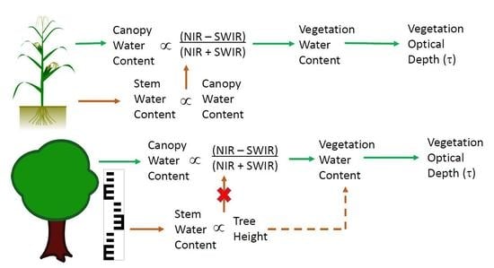
Figure 2.
Flowchart for regional simulations. Landsat 8 Operational Land Imager (OLI) data were used to calculate normalized difference infrared index (NDII), from which canopy water content (CWC) was estimated from previous research [19,20]. The land cover classification was the 2015 USDA-NASS Cropland Data Layer [44,45], which was used to determine the method for estimating stem water content. For herbaceous vegetation including crops, the algorithm is similar to the Soil Moisture Active Passive level 2 vegetation water content (VWC) data product [31,32], except that NDII is used instead of normalized difference vegetation index (NDVI). For woodland areas, stem water contents (SWC) was estimated assuming a mean canopy height of 18 m.

Figure 3.
Changes of leaf and stem water contents for maize and soybean plants over time. Slopes (ξ) were 2.86 and 1.71, R2 were 0.906 and 0.946, and root mean square errors (RMSE) were 43.0 and 3.3 for maize and soybean, respectively.
Figure 3.
Changes of leaf and stem water contents for maize and soybean plants over time. Slopes (ξ) were 2.86 and 1.71, R2 were 0.906 and 0.946, and root mean square errors (RMSE) were 43.0 and 3.3 for maize and soybean, respectively.

Figure 4.
(a) Color-infrared orthomosaic image and (b) digital surface elevation model derived from the airborne photogrammetric point cloud for box A in Figure 1. Whereas the ground surface was flat at about 20 m above sea level, the derived ground surface varied from 0 to 30 m.
Figure 4.
(a) Color-infrared orthomosaic image and (b) digital surface elevation model derived from the airborne photogrammetric point cloud for box A in Figure 1. Whereas the ground surface was flat at about 20 m above sea level, the derived ground surface varied from 0 to 30 m.

Figure 5.
(a) Color infrared orthomosaic and (b) digital surface elevation model derived from the airborne photogrammetric point cloud for box B in Figure 1. Colors of the digital surface model are the same as Figure 5b.

Figure 6.
Comparison of relative stand heights derived from airborne photogrammetric digital surface models with measured stand heights.
Figure 6.
Comparison of relative stand heights derived from airborne photogrammetric digital surface models with measured stand heights.

Figure 7.
(a) L8-OLI false color composite with red assigned Band 6 shortwave-infrared radiation (SWIR)-1, green assigned Band 5 near-infrared (NIR), and blue assigned Band 4 Red. (b) WV-3 false color composite with similar band assignments. Images cover box A in Figure 1.
Figure 7.
(a) L8-OLI false color composite with red assigned Band 6 shortwave-infrared radiation (SWIR)-1, green assigned Band 5 near-infrared (NIR), and blue assigned Band 4 Red. (b) WV-3 false color composite with similar band assignments. Images cover box A in Figure 1.

Figure 8.
(a) L8-OLI false color composite and (b) WV-3 false color composite for box B in Figure 1. Band assignments are the same as Figure 8.

Figure 9.
Normalized difference infrared index (NDII) from L8-OLI and WV-3 compared to (a) measured and (b) relative woodland stand heights. The Pearson correlation coefficients were not significant.
Figure 9.
Normalized difference infrared index (NDII) from L8-OLI and WV-3 compared to (a) measured and (b) relative woodland stand heights. The Pearson correlation coefficients were not significant.

Figure 10.
Relative errors of WindSat soil moisture retrievals at various vegetation water contents (VWC) after adding random noise to six brightness temperatures (vertical and horizontal polarizations at frequencies of 10.7, 18.7, and 37.0 GHz [40]. Maximum potential error was specified to be under 10%, therefore VWC needs to be less than 4 kg m−2.

Figure 11.
Stem water content as a function of stand height at 2 fractions of woodland land cover. The linear relationship was from Equation 5, which was empirically determined [50].
Figure 11.
Stem water content as a function of stand height at 2 fractions of woodland land cover. The linear relationship was from Equation 5, which was empirically determined [50].

Figure 12.
The 2015 Cropland Data Layer from the USDA National Agricultural Statistics Service [44,45] for Maryland’s Eastern Shore. The red rectangles show the two locations for acquisition of WV-3 satellite images and airborne color-infrared images.

Figure 13.
Simulated total vegetation water content (kg m−2) using L8-OLI data acquired on (a) 23 June 2015 and (b) 26 August 2015. Data were averaged over a 25-km diameter circle to simulate the spatial resolution of WindSat. The white outline shows the coastline and the yellow outline shows the boundary for the Choptank River watershed.


Table 1.
Spectral bands for Landsat 8 Operational Land Imager and WorldView-3.
| Landsat 8 Operational Land Imager (OLI) | WorldView-3 (WV-3) | ||||
|---|---|---|---|---|---|
| Band Name 1 | Wavelength (nm) | Resolution | Band Name | Wavelength (nm) | Resolution |
 | |||||
1 Includes band number, 2 Panchromatic (Pan), 3 Ground sample distance (GSD), 4 Resampled GSD from DigitalGlobe, 5 Near infrared (NIR), 6 Shortwave infrared (SWIR) band 1.
© 2018 by the authors. Licensee MDPI, Basel, Switzerland. This article is an open access article distributed under the terms and conditions of the Creative Commons Attribution (CC BY) license (http://creativecommons.org/licenses/by/4.0/).
Share and Cite
MDPI and ACS Style
Hunt, E.R.; Li, L.; Friedman, J.M.; Gaiser, P.W.; Twarog, E.; Cosh, M.H. Incorporation of Stem Water Content into Vegetation Optical Depth for Crops and Woodlands. Remote Sens. 2018, 10, 273. https://doi.org/10.3390/rs10020273
AMA Style
Hunt ER, Li L, Friedman JM, Gaiser PW, Twarog E, Cosh MH. Incorporation of Stem Water Content into Vegetation Optical Depth for Crops and Woodlands. Remote Sensing. 2018; 10(2):273. https://doi.org/10.3390/rs10020273
Chicago/Turabian StyleHunt, E. Raymond, Li Li, Jennifer M. Friedman, Peter W. Gaiser, Elizabeth Twarog, and Michael H. Cosh. 2018. "Incorporation of Stem Water Content into Vegetation Optical Depth for Crops and Woodlands" Remote Sensing 10, no. 2: 273. https://doi.org/10.3390/rs10020273
Note that from the first issue of 2016, this journal uses article numbers instead of page numbers. See further details here.