Using High-Resolution Airborne Data to Evaluate MERIS Atmospheric Correction and Intra-Pixel Variability in Nearshore Turbid Waters


1
Laboratoire de Planétologie et Géodynamique de Nantes (LPGN), UMR CNRS 6112, Université de Nantes, 2 rue de la Houssinière, 44322 Nantes, France
2
Mer Molécules Santé (MMS), EA 2160, Université de Nantes, 2 rue de la Houssinière, 44322 Nantes, France
*
Author to whom correspondence should be addressed.
Remote Sens. 2018, 10(2), 274; https://doi.org/10.3390/rs10020274
Submission received: 11 January 2018
/
Revised: 6 February 2018
/
Accepted: 8 February 2018
/
Published: 10 February 2018
(This article belongs to the Special Issue Remote Sensing in Coastal Zone Monitoring and Management—How Can Remote Sensing Challenge the Broad Spectrum of Temporal and Spatial Scales in Coastal Zone Dynamic?)
Abstract
:The implementation of accurate atmospheric correction is a prerequisite for satellite observation and water quality monitoring in coastal areas. The potential of the fast-line-of-sight atmospheric analysis of spectral hypercubes (FLAASH) was investigated here for the medium resolution imaging spectrometer (MERIS). As the comparison between discrete field sampling points and macro-scale satellite pixels is subject to spatial biases associated with small-scale spatial patchiness in the turbid and highly dynamic nearshore zone, an alternative approach was proposed here using high spatial resolution (1 m) airborne hyperspectral images as radiometric truthing references. While FLAASH was not optimal for moderately turbid offshore waters (suspended particulate matter (SPM) concentration < 50 g∙m−3), it yields satisfactory results in the 50–1500 g∙m−3 range, where MERIS standard atmospheric correction was subject to significant biases and failures. Due to the significant intra-pixel variability of SPM distribution in highly turbid areas, the acquisition of high resolution airborne images should be considered as a consistent strategy for the validation of medium resolution satellite remote sensing in the spatially heterogeneous and optically diverse nearshore waters.

1. Introduction
The monitoring of seawater constituents such as suspended particulate matter (SPM) and chlorophyll-a (Chl-a), a proxy of micro-algae, is crucial in estuaries and bays as their spatio-temporal variability is one of the main drivers of the functioning of coastal ecosystems [1]. The concentration of seawater constituents can be directly measured using field sampling, or indirectly derived from seawater optical properties [2] using bio-optical inversion algorithms. For example, SPM concentration can be derived from satellite observation of the water-leaving reflectance, ρw(λ), over a variety of spatio-temporal scales in coastal ecosystems [3,4]. One prerequisite for the remote sensing of in-water colored constituents is the accurate computation of surface reflectance from the top-of-atmosphere (TOA) satellite acquisition, and the accuracy of satellite observation therefore strongly depends on the atmospheric correction (AC).
First, the top-of-atmosphere radiance, LTOA(λ), detected by a satellite sensor is converted into TOA reflectance:
where ρTOA(λ) is the TOA reflectance, LTOA(λ) is the radiance measured by the sensor, E0(λ) is the solar spectral irradiance at TOA, and cosθ is the cosine of the sun zenith angle, θ. The water-leaving reflectance, ρw(λ), is then derived by solving the so-called radiative transfer equation:
where ρr(λ) is the reflectance resulting from Rayleigh scattering (air molecules), ρa(λ) is the reflectance from aerosols scattering, ρra(λ) is the reflectance due to multiple scattering between air molecules and aerosols, ρg(λ) is the glint reflectance due to the specular reflection of the solar radiation over the water surface, t is the atmospheric diffuse transmittance, and ρw(λ) is the ratio of the water-leaving radiance, Lw(λ), to the downwelling solar irradiance reaching the ocean’s surface, Ed(λ). While the reflectance due to molecular scattering is computed from Rayleigh formula, the contribution of aerosols is more challenging to evaluate, particularly over coastal waters.
ρTOA(λ) = ρr(λ) + ρa(λ) + ρra(λ) + ρg(λ) + t∙ρw(λ)
In clear oceanic waters, the decorrelation between ρTOA(λ) and ρw(λ) is usually performed using the black pixel assumption [5]. In the near infrared (NIR, 700–1000 nm) spectral domain, ρw(λ) is assumed to be zero, ρTOA(λ) is considered as the sole atmosphere contribution, and ρa(λ) + ρra(λ) can be directly measured at sensor level. Two NIR bands are then used to extrapolate the aerosol reflectance to the shorter wavelength using either the Angström exponent α(λ) [6] or the extrapolation parameter later introduced by Gordon and Wang [5]. The water-leaving reflectance is then computed over the whole visible and NIR spectrum, and can be used for the retrieval of seawater colored constituents.
The black pixel assumption is however restricted to clear waters whose optical properties are dominated by those of pure seawater and chlorophyll-a. In coastal and inland waters, the concentration of suspended particulate matter can be high enough to yield non-zero NIR ρw(λ) ([7], and invalidates the NIR black pixel assumption. Several AC methods have therefore been developed for coastal waters. Iterative schemes based on semi-analytical models of atmosphere and water-leaving reflectance improve the extrapolation of aerosol reflectance from the NIR to the shorter wavelength [8,9,10]. They are however still based on a NIR black pixel assumption, and can lead to underestimation of ρw(λ) in turbid waters. It was then proposed to switch the black pixel from the NIR to the short-wave infrared (SWIR) spectral region [11,12,13] because ρw(λ) is generally negligible over 1200 nm, even in extremely turbid areas where SPM concentration exceeds 300 g∙m−3 [11,14]. These algorithms are restricted to the sensors having SWIR bands with a sufficient signal-to-noise ratio (SNR) such as the operational land imager (OLI) on-board Landsat8, the moderate resolution imaging spectroradiometer (MODIS) on-board Aqua, or the multispectral instrument (MSI) on-board Sentinel2.
Unfortunately, the SWIR-AC algorithms are not applicable to the medium resolution imaging spectrometer (MERIS) on-board ENVISAT (2002–2012) or to the ocean and land color instrument (OLCI) on-board Sentinel3 (2016-present). For MERIS, other AC procedures have been developed and implemented in the MERIS ground segment processor (MEGS), including the so-called bright pixel atmospheric correction (BPAC, [15,16]). The BPAC identifies turbid pixels and corrects them from the residual water-leaving reflectance in the NIR prior the application of a standard clear water AC [17]. Similarly, the semi-analytical atmospheric and bio-optical processor (SAABIO) has been proposed as an alternative BPAC for MERIS [18], and validated in moderately turbid coastal waters [19]. Other AC methods perform a co-determination of the atmosphere and water contributions, such as the case2regional neural network algorithm (C2R, [20]) or the recent MEETC2 model [21]. These inversion methods however depend on the validity range of the atmosphere and seawater optical datasets used to supervise learning machines, and by now these methods have been trained with a global dataset, and not optimized for turbid coastal waters.
Another method of atmospheric correction, FLAASH (fast-line-of-sight atmospheric analysis of spectral hypercubes) [22], initially developed for land remote sensing, deserves to be further investigated in nearshore areas influenced by terrestrial aerosols [23]. FLAASH uses the MODTRAN (moderate resolution atmospheric transmission) radiative transfer code [24] to remove the atmosphere contribution from the at-sensor measured ρTOA(λ). MODTRAN uses spectral libraries at very high spectral resolution (<0.1 nm) to simulate the response of aerosols and molecules and generate atmospheric look up tables (LUT) that are implemented in FLAASH atmospheric model [24,25,26]. In nearshore areas, FLAASH has been successfully applied to airborne remote sensing over tidal flats [27,28], but has received little attention so far for ocean color remote sensing. Due to the very high resolution of MODTRAN atmospheric spectral libraries, FLAASH is applicable to a wide range of multispectral satellite sensors [29], including MERIS. The aim of the present study is to evaluate the accuracy of FLAASH for MERIS observation in a turbid coastal zone. The performance of FLAASH is compared with that of the MERIS standard atmospheric correction implemented in MEGS, as well as with the alternative SAABIO BPAC. An original validation approach is proposed here, based on the use of airborne hyperspectral images as truthing references instead of traditional in situ discrete field sampling, in order to avoid spatial biases associated with the small-scale (<1 m) spatial heterogeneity of SPM concentration in turbid nearshore waters.
2. Materials and Methods
2.1. Study Site
Bourgneuf Bay is a 340 km2 macrotidal bay along the French Atlantic coast, located south to the Loire estuary, and limited to the south by the island of Noirmoutier (Figure 1). It is an important site for shellfish aquaculture (mostly Pacific oysters), with an average annual production of about 5300 tons [30]. The surface of the intertidal zone is about 100 km2 with large mudflats in the northern part, and sandy tidal flats in the southern area. The concentration of suspended particulate matter (SPM) is generally high, and highly variable due to tidal resuspension, waves and currents. SPM concentration is generally higher than 100 g∙m−3 in the waters adjacent to the northern mudflats, and lower than 20 g∙m−3 in the southern area [31,32,33]. Phytoplankton growth is limited by too high SPM concentration in the most turbid waters, but high concentration of chlorophyll-a (Chl-a), over 10 mg∙m−3, has been documented in the vicinity of the tidal flats [31,34] and is due to the resuspension of benthic microalgae [35].
2.2. Remote Sensing Data and Processing
The remote sensing dataset consists in four pairs of airborne and MERIS images acquired within two hours of each other. The processing of airborne images was tailored, quality-controlled and validated using field measurements (see Section 2.2.1), so that the ground-truthed airborne surface reflectance was used as a reference to assess MERIS atmospheric correction accuracy and intra-pixel variability (see Section 2.3.4).
2.2.1. Processing of Airborne Hyperspectral Data
Between 2002 and 2012, a total of seven airborne hyperspectral images were acquired to monitor Bourgneuf Bay’s coastal zone at high resolution. Four airborne images were acquired concomitantly with MERIS overflights, and selected for the present study (Table 1). Three images were acquired over turbid waters in the northern area of the bay, and one image was acquired south to Noirmoutier Island over moderately turbid waters (Figure 1). Each airborne image is a cluster of several parallel flight lines acquired within 90 min, tailoring MERIS overflight by less than 2 h (Table 1). The airborne images were acquired from an Aeronef Piper Seneca II. Flight altitude was 2600 m, and the spatial resolution was 1 m. Radiometric measurements were performed in the visible and near infrared (VNIR), from 400 to 1000 nm, with a spectral resolution of 4.5 nm, using a hyperspectral camera (HySpex VNIR 1600, Norsk Elektro Optikk, Skedsmokorset, Norway).
The radiance at flight altitude, L*(λ), was computed following several steps: pre-flight sensor calibration using laboratory-measured reference, geometric calibration using field measurements (GPS data), and ortho-rectification using trajectory data. Images were georeferenced in the WGS84/UTM (Universal Transverse Mercator) zone 30 projection. The atmospheric correction was performed to compute the surface reflectance, ρ(λ), using the fast-line-of-sight atmospheric analysis of spectral hypercubes (FLAASH) algorithm implemented in ENVI (Harris Geospatial). Using MODTRAN (moderate resolution atmospheric transmission radiative transfer code) [24,36], FLAASH is implemented to solve the radiative transfer equation including the effects of molecular and particulate absorption and scattering, surface reflection and emission, and solar illumination, on a pixel-by-pixel basis:
where L* is the spectral radiance measured at flight altitude for a given pixel, ρ is the surface reflectance at the same pixel, ρe is an average surface reflectance for the neighboring pixels that accounts for adjacency effects, S is the spherical albedo of the atmosphere, A and B are coefficients that depend on atmospheric and geometric conditions, and La* is the radiance backscattered by the atmosphere. For the present study, the atmosphere was modeled using a US standard atmospheric model with a visibility of 40 km, and a maritime aerosol model that considers both the influence of oceanic winds and the presence of aerosols from terrestrial origins. The water vapor amount was retrieved using the narrow water absorption band at 840 nm (Table 2). FLAASH parameterization was optimized after several trials and validated using ground references (Figure 2). The remote-sensing reflectance, Rrs(λ), corresponding to the surface reflectance in the direction of the sensor’s viewing angle, was then computed using the standard definition:
L* = A ρ/(1 − ρe S) + B ρe/(1 − ρe S) + La*
ρ(λ) = π Rrs(λ)
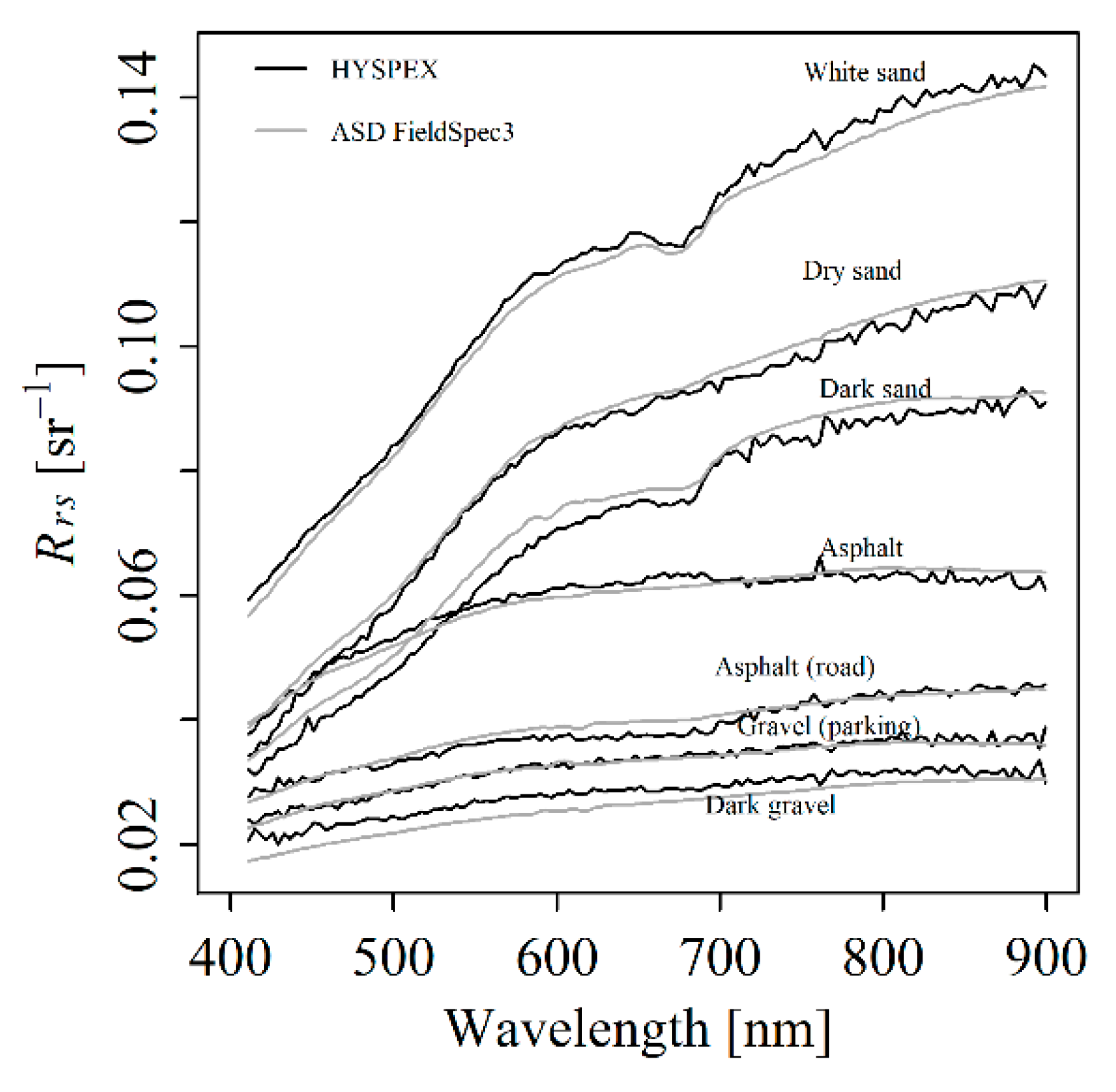
For each airborne image, residual errors were then removed using the ground control points (GCP) method described in [36]. The airborne-retrieved surface reflectance was eventually adjusted to the reflectance of a single white reference (namely a ~1 m × 1 m homogeneous area of white dry sand) measured using a hyperspectral ASD FieldSpec3 spectrometer. Using this ground reference, a simple ratio was applied to the whole scene. The fact that a single ratio proved satisfactory over a variety of surfaces (Figure 2) suggested that the mismatch between field and airborne-derived reflectance was low, and mainly due to a constant instrumental drift of the camera. The adjustment was not applied to MERIS data (see Section 2.2.2) whose calibration gains have been regularly controlled [37]. Additional in situ Rrs(λ) spectra of a variety of ground reference targets (from white sand to dark gravel) were performed to ground-truth airborne data on 21–22 September 2009 (Figure 2). For these reference targets, the root mean square error between the field- and airborne-derived Rrs(λ) was less than 0.008 sr−1. Post processing was then performed to improve the signal to noise ratio (SNR). A minimum noise fraction (MNF) was applied on a 20 spectral bands basis, thus reducing the spectral range between 400 and 900 nm. A low-pass filter was eventually applied to remove the remaining residual noise.
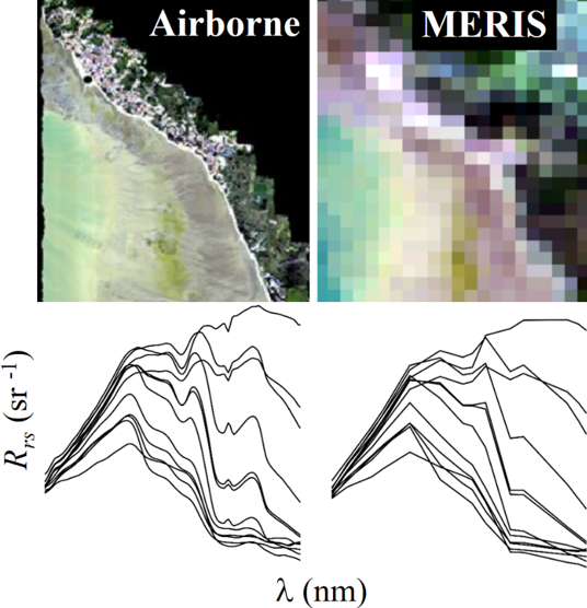
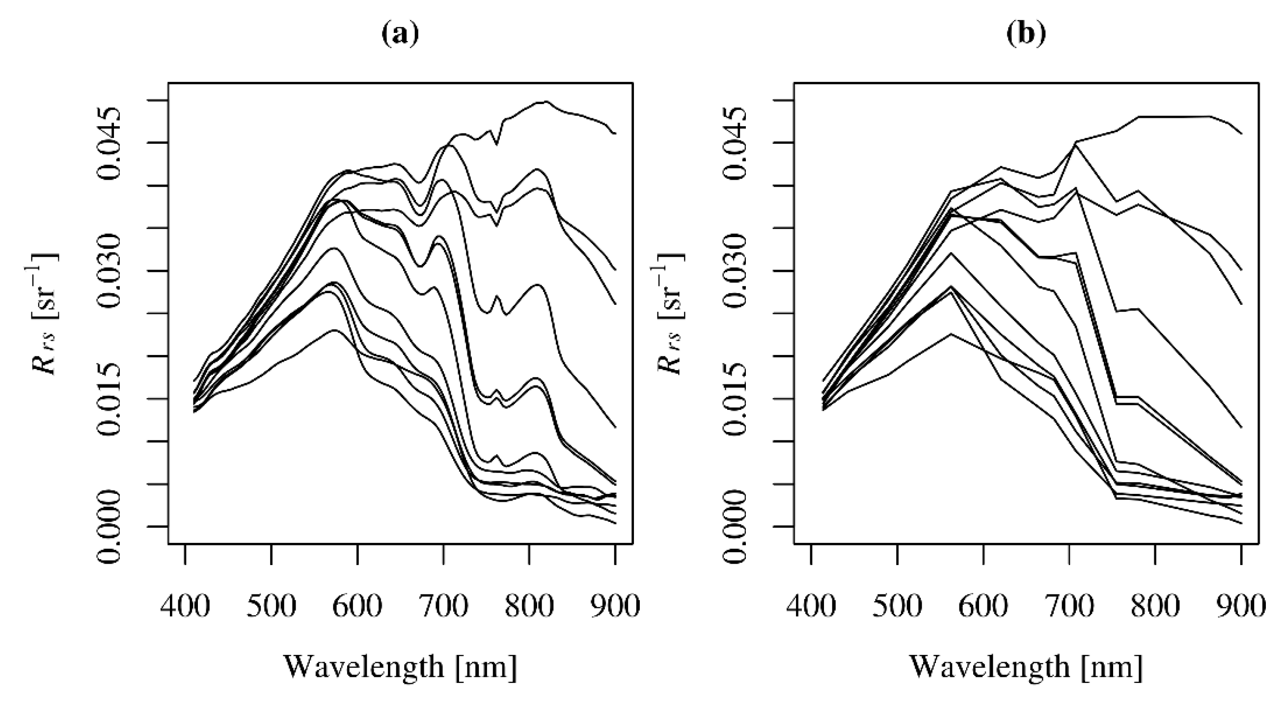
The quality-controlled, field-adjusted, and ground-truthed airborne surface reflectance data were then used as a substitute for field measurements to evaluate the accuracy of MERIS processing. Such an approach has the notable advantage of avoiding spatial scale discrepancy when comparing field sampling of an isolated point (observed surface is <10 cm) with satellite observation over macro-pixels (observed surface is >100 m). For the consistency of the HySpex–MERIS comparison, the high-resolution airborne data were spectrally downgraded at MERIS spectral resolution (15 bands) using its spectral response function (SRF) (Figure 3), and spatially downscaled from 1 to 300 m using a pixel aggregating method (Figure 4).
2.2.2. MERIS Data
The medium resolution imaging spectrometer (MERIS) has been operational from 2002 to 2012 on-board the environment satellite ENVISAT of the European space agency (ESA). MERIS had 15 spectral channels in the visible and near infrared, from 412 to 900 nm, with a spectral resolution between 3.75 and 20 nm, and an average bandwidth of 10 nm. For the present study, four images at full resolution (FR) acquired the same day than the airborne images were selected (Table 1). Top-of-atmosphere (TOA) MERIS FR data were downloaded from the MERCI web portal (http://merisfrs-merci-ds.eo.esa.int/merci/queryProducts.do), and processed using ENVI. MERIS images were georeferenced in WGS84/UTM30 and co-located with the airborne data. Numerical count (dimensionless radiance floating point value) was converted into TOA radiance, LTOA(λ) [in μW∙cm−2 nm−1∙sr−1], using the scale factors provided in the auxiliary data. As for the airborne data, the FLAASH atmospheric correction was used to compute ρ(λ) using the US standard atmospheric model with a visibility of 40 km, and a maritime aerosol model (Table 2). The sole difference between the parameterization of FLAASH for HySpex and MERIS is that no water vapor retrieval was performed for MERIS due to its too low spectral resolution in the NIR, and to the absence of a narrow spectral band at 840 nm. The water vapor amount was estimated equal to 1.42 g∙cm−2 using the atmosphere model, and uniformly applied to the whole MERIS scene. The band centered at 761 nm was removed: it corresponds to a maximum of oxygen absorption, and is strongly affected by the scattering of high clouds (cirrus). Contrary to the airborne data, MERIS data were not ground-controlled, and the surface reflectance was not adjusted after the AC. The size of the white reference (1 m) used in the post-AC adjustment is indeed incompatible with the size of a 300 m pixel.
In addition to FLAASH, two other AC methods were tested. The AC of the MERIS ground segment prototype processor (MEGS 8.1) was applied to compute the standard reflectance product. MEGS includes a bright pixel atmospheric correction (BPAC) that removes the residual marine signal in the NIR for turbid water pixels [16], before applying a standard atmospheric correction developed for clear oceanic waters [17]. Second, MERIS standard processing was compared with an alternative version of MEGS 8.1 in which the initial BPAC is replaced by the SAABIO (semi-analytical atmospheric and bio-optical processor) BPAC [18,19]. In the initial BPAC [16], turbid pixels are identified using a threshold on ρw(709 nm), and for these pixels the water-leaving reflectance is computed using iterative non-linear equations, and removed from the aerosol reflectance at 779 and 865 nm. The aerosol reflectance is then extrapolated from the NIR to the shorter wavelengths, and ρw(λ) is eventually estimated over the whole VNIR spectral range. The SAABIO BPAC is based on the same principle, but two additional bands at 560 and 620 nm are included to improve the extrapolation of the aerosol reflectance from the NIR to the visible bands [18]. Both MEGS 8.1 and SAABIO MERIS FR data were downloaded from the Kalicôtier web portal (http://kalicotier.gis-cooc.org). MERIS surface reflectance data were then cropped to the size of the airborne scene, and the three MERIS surface reflectance products (namely the FLAASH, MEGS, and SAABIO) were compared with the co-located airborne surface reflectance data.
2.3. Comparison between HySpex Airborne and MERIS Satellite Data
The FLAASH atmospheric correction makes it possible to retrieve the surface reflectance over land and water, whereas the AC used in MEGS and SAABIO is applicable only over water. As the remote sensing dataset encompasses both land (mudflats) and water, each pixel was identified and classified (Section 2.3.1) before the evaluation of the different atmospheric corrections. For the marine pixels, three turbidity classes were distinguished to assess the performance of MERIS processing in moderately turbid, very turbid, and extremely turbid waters (Section 2.3.2). Airborne vs. satellite comparison was then performed in each turbidity class and quantified using standard metrics (Section 2.3.3). Over water, the uncertainty of MERIS AC was then eventually compared with MERIS intra-pixel variability, which was quantified using airborne data at native spatial resolution (Section 2.3.4).
2.3.1. Identification of Land and Water Pixels
In the intertidal zone, the identification of land and water pixels is challenging because the frontier between very turbid waters and wet mudflats is not easy to detect. Due to the absence of short wave infrared (SWIR) bands in both HySpex and MERIS data, the commonly applied normalized differential water index (NDWI, [38]) could not be used in the present study. Instead, the identification of microphytobenthos (benthic microalgae forming biofilms at sediment’s surface during low tide) was used as a proxy of mudflat detection. Two indexes were used to detect microphytobenthos (MPB), the normalized differential vegetation index (NDVI, [39]), and the microphytobenthos index (MPBI, [28]), which were, respectively, computed as:
The NDVI is widely used in land remote sensing to detect vegetation, which is characterized by the red absorption band of chlorophyll-a at 675 nm, and by a drastic change in the reflectance spectral slope between the red and the NIR. Here, a NDVI threshold of 0.5 was applied to distinguish MPB biofilms from terrestrial vegetation and macroalgae [40]. Whereas the NDVI detects all green biomass, the MPBI is more specific to the spectral features of benthic microalgae, characterized by a reflectance maximum at 560 nm, and two minima at 490 and 675 nm. Therefore, MPB detection was enhanced by the application of a MPBI threshold, corresponding to pixels for which MPBI > NDVI [40]. The combination of the NDVI and MPBI thresholds improved MPB detection, which was used here as a proxy of mudflat detection. Water was then distinguished from mudflat using negative NDVI values. As the airborne and MERIS satellite images were acquired on the same day but not exactly at the same time, a few pixels were identified as water on the satellite images, and as land on the airborne images (and inversely). To avoid any confusion, the mudflat and water indexes were computed for both MERIS and airborne images, and only the pixels meeting the above-mentioned criteria on both images were selected.
2.3.2. Classification of Water Pixels
Water pixels were then sorted out according to SPM concentration in order to investigate the influence of turbidity on AC performance. SPM concentration was computed from HySpex airborne water-leaving reflectance using a multi-conditional algorithm recently developed for Bourgneuf Bay and validated along a wide range of turbidity [41]. Three turbidity classes were defined according to the range of SPM concentration (Table 3). Class 1 corresponds to moderately turbid water (SPM < 50 g∙m−3), class 2 to very turbid water (50 < SPM < 200 g∙m−3), and class 3 to extremely turbid waters (SPM > 200 g∙m−3). Class 1 corresponded to the area south to the island of Noirmoutier, whereas classes 2 and 3 corresponded to the northern mudflat (Figure 1). The thresholds between the three classes were set up so that each class has approximately the same number of pixels (Table 3).
2.3.3. Evaluation of MERIS Atmospheric Correction Using Airborne Macro-Pixel Data
As explained earlier, ground-truthed airborne HySpex data downscaled at MERIS spatial and spectral resolutions were used as reference dataset to evaluate the accuracy of MERIS atmospheric correction. The evaluation was performed separately for the land (mudflat) and water pixels, and within each turbidity class for the water pixels. Two standard metrics, the spectral root mean square error, RMSE(λ), and the spectral relative root mean square error, RRMSE(λ), were computed between the HySpex and MERIS remote-sensing reflectance Rrs(λ):
where Yi corresponds to MERIS Rrs(λ) at a given spectral band, Xi corresponds to HySpex Rrs(λ) of the corresponding macro-pixel at the same spectral band, and N is the number of points in each class (see Table 3).
For each macro-pixel, the spectrally averaged RMSE, hereafter noted RMSEAC, was also computed:
where Yj is MERIS Rrs(λ) at a spectral band j, Xj is the reflectance of the corresponding HySpex macro-pixel at spectral band j, and M is the number of spectral bands (i.e., M = 15). The subscript “AC” was introduced in order to differentiate the RMSE due to atmospheric correction against the RMSE due to intra-pixel spatial variability (see below).
2.3.4. Evaluation of Intra-Pixel Spatial Variability (300 m)
For each 300 m macro-pixel simulated from the airborne image, the intra-pixel variability was evaluated using the corresponding 90,000 airborne pixels at native spatial resolution (1 m). The intra-pixel RMSE, hereafter referred as RMSEPIX, was defined as:
where Yj,k is HySpex Rrs(λ) at a spectral band j, for a given pixel k at 1 m resolution, Xj corresponds to the reflectance of the corresponding macro-pixel at spectral band j, M is the number of spectral bands (i.e., M = 15), and P is the number of high-resolution pixels within a macro-pixel (i.e., P = 90,000).
3. Results
3.1. Performance of MERIS Atmospheric Correction
3.1.1. Atmospheric Correction over Land (Mudflat)
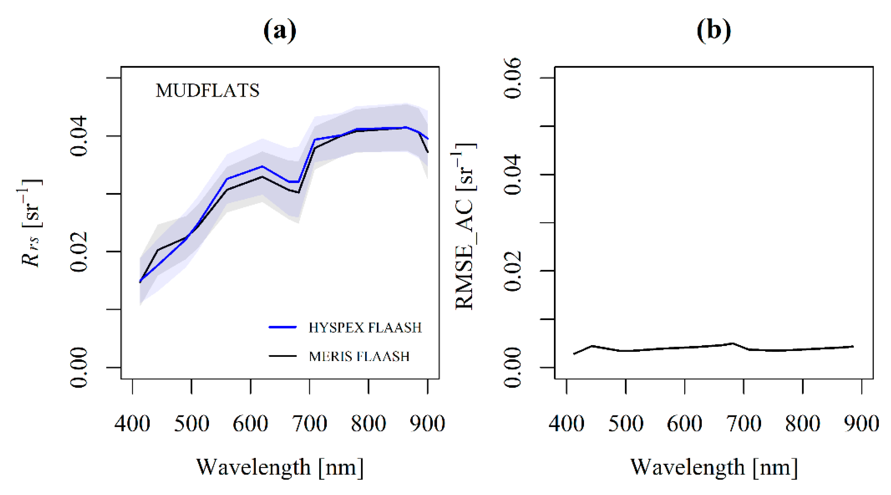
Over land, the standard deviation of the airborne Rrs(λ) spectra is low, around 0.003 sr−1, due to the radiometric homogeneity of the mudflat (Figure 5a). The averaged spectrum is typical of mud covered by a biofilm of benthic microalgae with a trough near 675 nm resulting from the red absorption by chlorophyll-a [42]. Due to the absence of Chl-a reflectance in the NIR, the airborne-derived Rrs(λ) is equal to the spectral response of the mud substrate between 700 and 900 nm [27,28]. Over the wet mudflat, the NIR plateau (0.04 sr−1) is lower than usually observed on dry mud (0.05 sr−1). The corresponding MERIS spectra are very similar in shape, intensity, and standard deviation. The RMSE between the mudflat-averaged HySpex and MERIS Rrs(λ) is spectrally flat and consistently lower than 0.004 sr−1 (Figure 5b), with an average value of 0.0035 sr−1 (Table 4).
3.1.2. Atmospheric Correction over Water
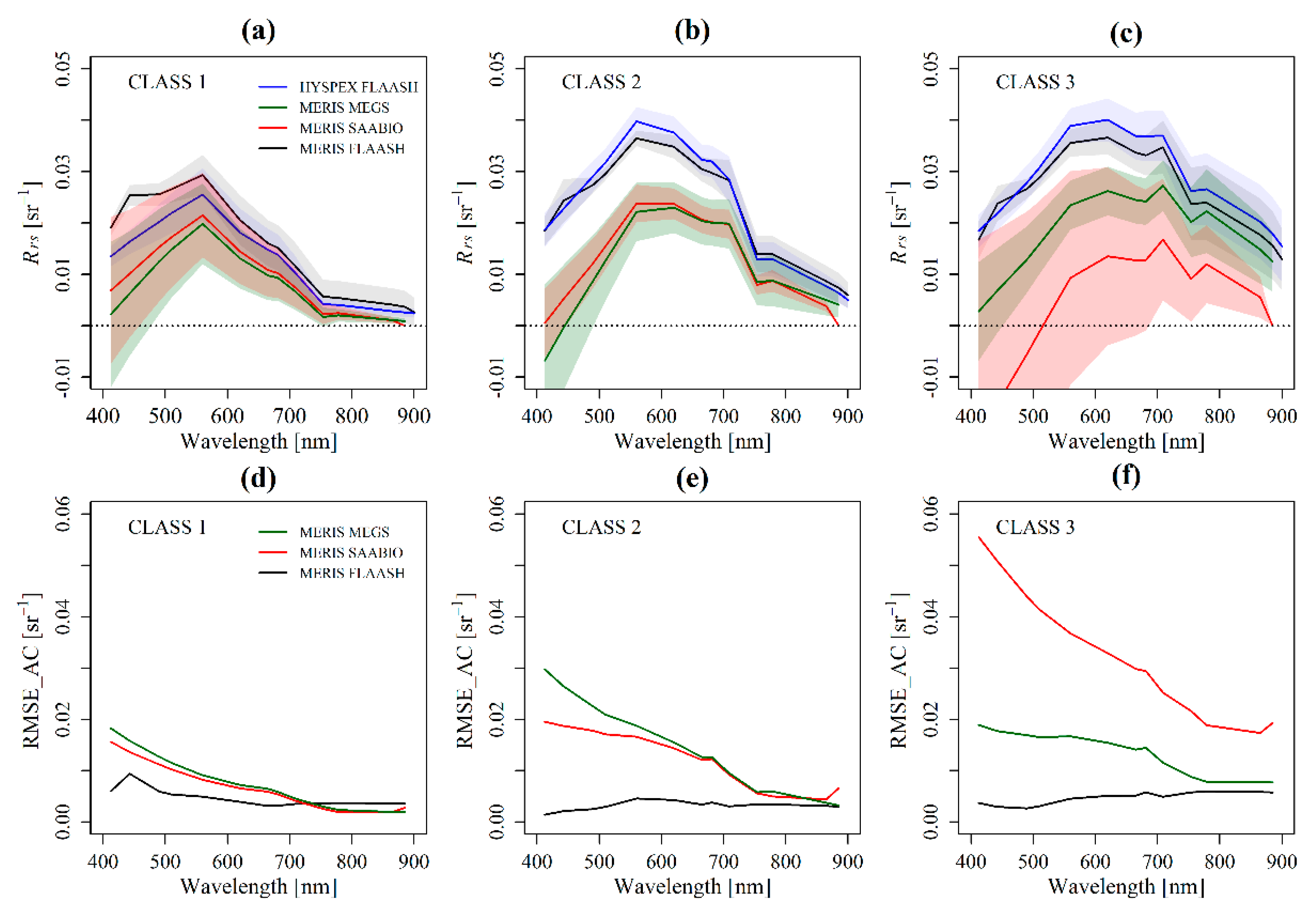
Over water, the airborne Rrs(λ) spectra consistently display the typical spectral features of Bourgneuf Bay turbid areas [33,34]. The spectral shape, intensity, and standard deviation of the Rrs(λ) spectra are very variable from one class to another (Figure 6a–c). Between class 1 (moderately turbid) and class 3 (extremely turbid), the standard deviation increases from 0.002 to 0.007 sr−1. In moderately turbid waters (class 1, Figure 6a), the averaged spectrum regularly increases from the blue to the green, and reaches a maximum of 0.025 sr−1 near 560 nm. Rrs(λ) then decreases at longer wavelengths, with a steeper slope in the red than in the NIR, where Rrs(λ) reaches a minimum of about 0.003 sr−1 at 900 nm. The spectral signature of the chlorophyll-a absorption band near 675 nm is hardly visible. In very turbid waters (class 2, Figure 6b), Rrs(λ) has a similar spectral shape in the blue and green, but the green maximum is higher (0.04 sr−1) than in class 1. In the red and NIR, Rrs(λ) displays typical features of turbid intertidal waters characterized by non-zero reflectance, and the minimum reaches 0.005 sr−1 near 900 nm. The spectral signature of chlorophyll-a near 675 nm is more visible than in class 1, and is attributable to the (tidal) resuspension of benthic microalgae. In extremely turbid waters (class 3, Figure 6c), Rrs(λ) exhibits very high red and NIR value (minimum Rrs(λ) near 900 nm is as high as 0.016 sr−1), and a pronounced chlorophyll-a signature near 675 nm.
With respect to the ground-truthed airborne data, the performance of the tested MERIS atmospheric corrections is unequal, and depends on the turbidity range (Figure 6). Compared to the airborne reference, the FLAASH-derived Rrs(λ) is overestimated by about 81% in the less turbid site off Noirmoutier island (Table 4). When SPM concentration exceeds 50 g∙m−3 (for class 2) and 200 g∙m−3 (for class 3), FLAASH becomes more accurate, and the relative RMSE between the MERIS and airborne Rrs(λ) spectra drops to 22% and 16% for classes 2 and 3, respectively. Despite an unexpected bump at 442 nm, the MERIS spectra Rrs(λ) consistently exhibit the features of turbid waters, such as the increase in the red and NIR at higher SPM concentration. The RMSE remains spectrally stable and consistently below 0.01 sr−1, whatever the range of turbidity (Figure 6d–f). The standard deviation around the averaged spectrum is similar with that of the airborne reference, and it is noteworthy that the application of FLAASH does not yield negative value.
The atmospheric correction implemented in MEGS yield several errors in the observed turbid waters. MEGS-derived Rrs(λ) is systematically lower by about 50% than the airborne reference (Figure 6a–c, and Table 4). The RMSE is wavelength-dependent, with a decreasing trend at longer wavelengths (Figure 6d–f). The RMSE is >0.01 sr−1 in the blue and green spectral bands (Figure 6d–f). The standard deviation is quite high, and negative values are observed at the shorter wavelengths.
The SAABIO AC performs similarly than MEGS in classes 1 and 2 (Table 4, Figure 6). The accuracy and robustness of the SAABIO AC however dramatically degrades when the SPM concentration exceeds 200 g∙m−3. In extremely turbid waters, the SAABIO-derived Rrs(λ) shows inconsistent spectral shape, negative values, and high instability (Figure 6c). The RMSE is high and wavelength-dependent, and increases from 0.055 to 0.02 sr−1 between 412 and 900 nm (Figure 6f). In this class of turbidity, the overall RMSE exceeds 100% (Table 4).
3.1.3. Influence of Turbidity on Atmospheric Correction
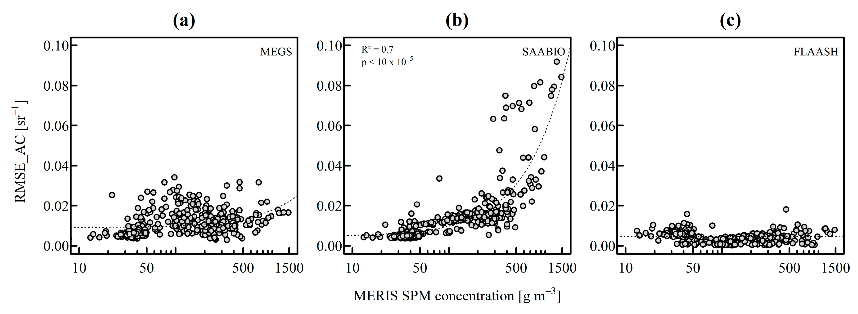
To better appraise the influence of turbidity on MERIS level 2 processing, SPM concentration was plotted against the RMSE of the tested atmospheric corrections (Figure 7). For the MEGS-derived Rrs(λ), the spectrally averaged RMSE varies between 0.005 and 0.035 sr−1, and is mostly independent of SPM concentration (Figure 7a). For the SAABIO-derived Rrs(λ), the RMSE dramatically increases with SPM concentration, exponentially varying from 0.005 to 0.1 sr−1 between 10 and 1500 g∙m−3 (Figure 7b). For the FLAASH-derived Rrs(λ), the RMSE remains systematically below 0.02 sr−1, with most points below 0.01 sr−1 whatever the SPM range (Figure 7c).
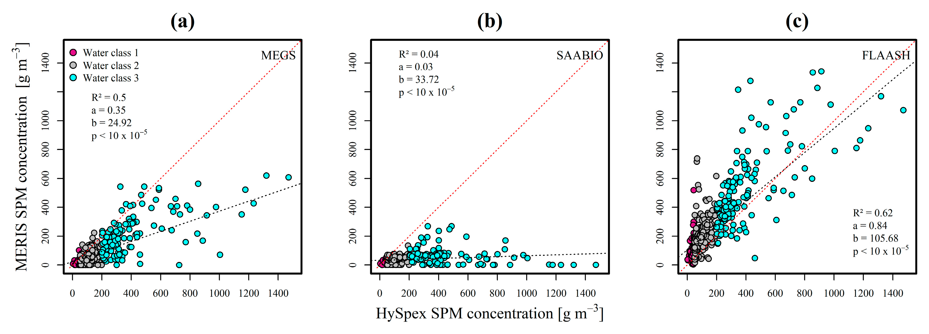
The influence of turbidity on atmospheric correction errors is further illustrated when looking at the matchups between airborne- and satellite-derived SPM products (Figure 8).
Overall, the inaccuracies are transmitted from the water-leaving reflectance to the retrieval of SPM concentration. Due to the reflectance underestimation, MEGS-derived SPM concentration is almost systematically lower by a factor of 2 than its airborne counterpart (Figure 8a). The underestimation is even worse for SAABIO (Figure 8b). Furthermore, SAABIO-and MEGS-derived SPM saturate when SPM concentration exceeds 200 and 600 g∙m−3, respectively. The SPM matchup significantly improves when the FLAASH atmospheric correction is applied (Figure 8c). The underestimation and saturation issues are avoided, and a significant linear relationship between airborne-derived and MERIS-derived SPM concentration is found all over the range of SPM concentration.
3.2. Evaluation of MERIS Intra-Pixel Variability and Comparison with AC Uncertainty
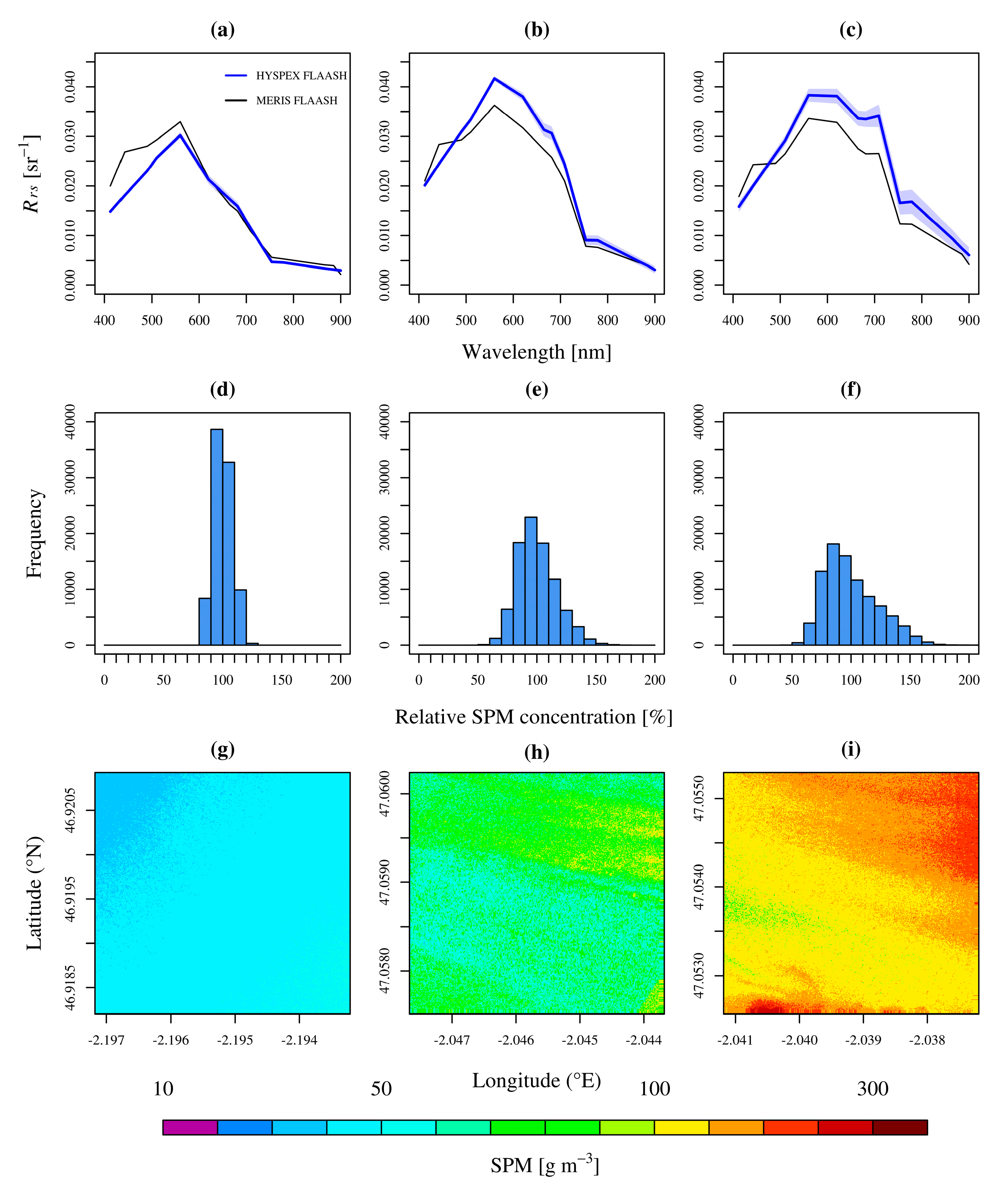
Three examples representative of moderately, highly and extremely turbid macro-pixels were selected to illustrate the amount of spatial variability within a 300 m MERIS pixel (Figure 9).
For each macro-pixel, the intra-pixel variability was evaluated using the corresponding 90,000 airborne pixels at native spatial resolution (1 m). Small-scale patchiness is clearly apparent on these examples, and increases with turbidity (Figure 9g–i). Within the moderately turbid macro-pixel, SPM concentration remains around 50 g∙m−3 (Figure 9g), with a percent deviation of about ±25% (Figure 9d). The range of SPM variability increases within the very turbid and extremely turbid macro-pixels, for which SPM concentration ranges between 50 and 170 g∙m−3 (Figure 9h), and between 50 and 260 g∙m−3 (Figure 9i), respectively. For the moderately turbid and very turbid examples, SPM intra-pixel variability follows a Gaussian law (Figure 9d,e), whereas the distribution of SPM concentration within the extremely turbid macro-pixel is shifted to the right (Figure 9f). For these three examples, the RMSE due to atmospheric correction uncertainty is one order higher than the standard deviation due to the intra-pixel spatial variability (respectively 0.0005, 0.0008 and 0.0015 sr−1 in Figure 9a–c).
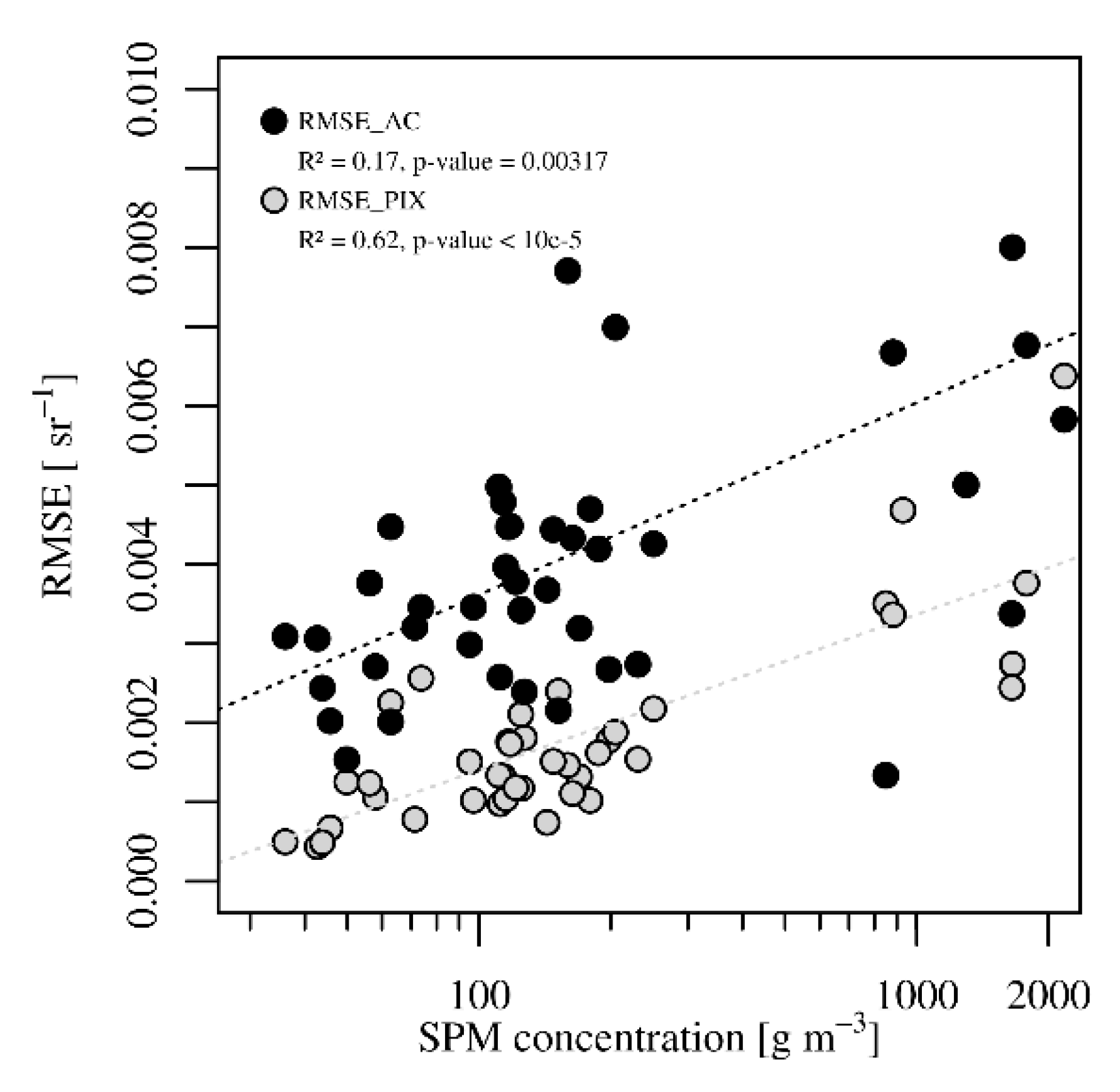
The RMSE due to the uncertainties of the FLAASH atmospheric correction (RMSEAC) was further compared with the RMSE due to intra-pixel variability (RMSEPIX) on 40 selected macro-pixels over a wide range of SPM concentration (Figure 10). Both RMSEs increase with SPM concentration, but RMSEAC is less dependent on the turbidity than RMSEPIX (r2 = 0.17, against r2 = 0.62). Interestingly, as RMSEPIX increases with turbidity more rapidly than RMSEAC, the difference between the two RMSEs is lower at higher SPM concentration. When SPM concentration exceeds 500 g∙m−3, the RMSEAC to RMSEPIX ratio can be as low as 15%, whereas it is generally higher than 100% in the 30–300 g∙m−3 range.
4. Discussion
4.1. Validity Range of AC Algorithms
In the present study, the atmospheric corrections implemented in MEGS and SAABIO were suitable for moderately turbid coastal waters, for which a limit could be approximately set to SPM concentration < 50 g∙m−3. In this range of SPM concentration, their RMSE is lower than 0.02 sr−1, and they provided the most accurate results in the NIR spectral domain (Figure 6b). At higher turbidity, and particularly when SPM concentration exceeds 100 g∙m−3, both methods yield several errors including Rrs(λ) underestimation, retrieval of negative Rrs(λ), and spatial instability, as shown by the high standard deviation of the Rrs(λ) spectra within a single turbidity class (Figure 6f). These limitations were previously documented in the literature, and partly attributed to the overestimation of the aerosol optical thickness at 865 nm [43]. Due to the extrapolation from the NIR to the visible, any error in the inversion of the aerosol optical properties will be transmitted and exponentially amplified at the shorter wavelengths. Another source of error is associated with the range of validity of the bio-optical model implemented in the BPAC. The marine reflectance model implemented in SAABIO has been developed using a large dataset of in situ measurements acquired over a variety of coastal waters in Europe [44,45], and validated in moderately turbid coastal waters for a range of SPM concentration < 100 g∙m−3 [19]. This upper limit, frequently surpassed in Bourgneuf Bay, is not adapted to turbid intertidal zones and coastal waters adjacent to mudflats.
In contrast, FLAASH provided satisfactory results in the turbid nearshore waters, whereas its performance in the moderately turbid waters off Noirmoutier was equivalent to that of the two other ACs. Contrary to the two other ACs, in FLAASH, there is no assumption on the optical properties of the suspended colored constituents, and the atmospheric model is independent of the marine signal. Due to the optical diversity and small-scale spatial variability of nearshore waters, the modeling of the seawater optical properties is very challenging [46,47], and subject to many uncertainties. In this context, FLAASH-derived surface reflectance is less exposed to biases and artefacts than the two other approaches.
The main limitation of FLAASH is the assumption of a uniform atmosphere over the whole scene. FLAASH is consequently valid only over areas where the atmosphere and aerosol models are appropriate. In the present study, a maritime aerosol model was selected. Such an aerosol model, that considers both the influence of oceanic air masses and the presence of aerosols of terrestrial origin, is by definition more appropriate nearshore than offshore. In this context, it is not surprising that FLAASH yields accurate results in Bourgneuf Bay, a semi-enclosed environment where the atmosphere contains a notable proportion of aerosols from terrestrial origin. Similarly, the moderate performance off Noirmoutier Island is not surprising, as the area is less influenced by continental air masses than Bourgneuf Bay’s mudflats. In summary, as FLAASH can be parameterized for coastal areas influenced by both terrestrial and marine aerosol model, it is particularly adapted to nearshore areas, which are generally also very turbid due to sediment resuspension in intertidal mudflats.
4.2. Transmission of AC Errors in SPM Retrieval
The present study highlighted the transmission of AC errors to the computation of SPM concentration. Here, SPM concentration was computed using a multi-conditional algorithm, specifically calibrated and validated for Bourgneuf Bay and the Loire estuary [41]. The errors in SPM retrieval are therefore mostly due to AC failures, rather than to uncertainties in the bio-optical algorithm. Similarly, other bio-geo-physical parameters derived from water-leaving reflectance are known to be affected by AC errors, particularly when they require the use of blue spectral bands, such as the diverse ocean color algorithms [48,49] used to retrieve Chl-a concentration.
Interestingly, for a given atmospheric correction, the SPM-retrieval error was lower with the band-switching algorithm than with a simple NIR-to-red band ratio algorithm [33] (data not shown). Multi-conditional or blending algorithms [41,50,51] that optimize the selection of satellite spectral bands are consequently expected to be more robust to AC failures in turbid coastal waters.
4.3. Other Advantages of FLAASH
Besides its ability to satisfactorily retrieve Rrs(λ) and SPM concentration in the highly turbid nearshore waters, FLAASH has also two main other advantages for the remote sensing of mudflats. First, the same AC can be used over water and land, which makes it possible to use a single AC processing when studying the land–water continuum in intertidal ecosystems. More broadly, the development of land–water AC could help improving the monitoring of inland, transitional, coastal and shelf–sea interconnected systems [4]. Second, as the use of MODTRAN makes it possible to simulate the spectral response of atmospheric molecules and aerosols at extremely high spectral resolution, FLAASH can be applied to a variety of multispectral satellite sensors. For example, FLAASH was used for a MODIS/Landsat/Formosat study of SPM distribution in a US estuarine system [29], and for the analysis of benthic microalgae spatial interactions using long-term Landsat and SPOT time-series in an intertidal ecosystem [52]. The present study confirmed the efficiency of FLAASH for the processing of hyperspectral airborne data as well as MERIS multispectral satellite data, and FLAASH can be equally applied to many other airborne and satellite sensors. The reliability of FLAASH for MERIS makes available a 10-years data archive (2002–2012) to study intertidal ecosystems, and the expected applicability of FLAASH to Sentinel3’s OLCI would allow extending nearshore environmental monitoring to the next decade.
4.4. Airborne Data, Spatial Scales, and Satellite Validation
Coastal areas are very dynamic media characterized by a wide range of spatial and temporal variability due to wind, waves, river flow, tides, and bathymetry changes [53]. In Bourgneuf Bay’s nearshore waters, the variability in the concentration of SPM and of other colored constituents is mainly driven by tidal variability and bathymetry changes [33,34]. As turbidity varies due to tidal cycles of erosion, resuspension and redeposition, the most turbid areas generally correspond to the areas where hydrodynamics and/or tidal currents are maximal. In such turbid maxima, SPM spatial distribution is highly heterogeneous due to plumes and stretches of high-concentrated mud suspensions, and the associated surface patchiness has spatial scales varying from <1 cm to >10 m. This entails two corollaries for the remote sensing of turbid areas: (i) satellite observation is required at high spatial resolution to quantify SPM dynamics without biases [54]; and (ii) SPM patchiness should be taken into account in validation strategy and in situ measurement acquisition protocol [55].
As far as validation is concerned, the degree of MERIS intra-pixel spatial variability reported in the present study, especially in highly turbid waters, questions about the pertinence of discrete in situ measurements commonly used to validate medium resolution satellite data. In contrast, airborne observation can resolve the scale issue, as the very high resolution airborne images can be downscaled at the spatial resolution of any targeted satellite sensor. Ideally, the airborne acquisition should be synchronous with satellite overflight to avoid any temporal bias. In practice, such constraint is difficult to achieve. In the present study, the time difference between airborne and satellite acquisition was lower than 2 h, and we did not see any significant influence of time difference on Rrs(λ) RMSE, but our dataset was not designed to investigate temporal variability. The use of continuous acquisition platforms or buoys improves the temporal representativeness of observation [55], but such measurements are less useful to validate satellite images over spatially heterogeneous water masses. Ideally, fixed-station time-series should be completed by airborne data, as it encompasses much larger areas, including zones that are difficult to instrument or to sample in the field. Beside the quantification of intra-pixel variability and the resolution of the scale issue, a validation method based on airborne acquisition also significantly increases the number of reflectance measurements available for validation purpose. As an example, in the present study, about 400 MERIS-like macro-pixels were available with only four airborne images. In contrast, a huge field sampling effort would be needed to equal the number of Rrs(λ) spectra acquired during a single airborne overflight. Even though the acquisition of airborne data is technically demanding, it should be considered as an alternative strategy for the validation of satellite observation in highly dynamics and optically heterogeneous coastal areas.
5. Conclusions
The performance of the FLAASH, MEGS and SAABIO atmospheric corrections were evaluated for MERIS remote sensing in coastal turbid waters. As the SPM spatial distribution was characterized by significant intra-pixel variability and small-scale surface patchiness in the most turbid areas, the validation method was based on the use of high resolution airborne hyperspectral images instead of traditional in situ matchup points. Airborne images indeed cover optically diverse and large areas, provide large numbers of radiometric measurements, and offer a consistent intermediate scale between macro-scale satellite observation and local field measurements. In moderately turbid waters (SPM concentration from 10 to 50 g∙m−3), MEGS and SAABIO provided the most accurate results, with a reflectance RMSE lower than 0.02 and 0.01 sr−1 in the blue-green, and red-NIR spectral domains, respectively. For the nearshore turbid waters (SPM concentration from 50 to 1500 g∙m−3), both methods exhibited significant failures such as RMSE spectral dependency, Rrs(λ) and SPM underestimation, and Rrs(λ) negative retrieval in the blue-green spectral bands. In contrast, FLAASH yields satisfactory results in turbid nearshore waters, with a reflectance RMSE consistently lower than 0.01 sr−1 all over the VNIR spectrum and whatever the turbidity range. Due to its multi-sensor plasticity and ability to retrieve surface reflectance over land as well as nearshore waters influenced by terrestrial aerosols, FLAASH could be consistently applied to a variety of satellite missions for the observation of the land–ocean continuum.
Data Availability
MERIS data are freely distributed by ESA. Airborne RGB images are available online (http://ids.osuna.univ-nantes.fr/). Raw airborne data are available upon request.
Acknowledgments
The ASD field spectroradiometer and HySpex hyperspectral camera of the LPG were funded by the “contrat de projet état région” (CPER) in Pays de la Loire (R 51_p6 2007–2013) with European regional development fund (ERDF). Airborne hyperspectral data were acquired in the frame of HySens and of the Geopal regional program for coastal observation, funded by the Region Pays de Loire and coordinated by the “observatoire des sciences de l’univers de Nantes Atlantique” (OSUNA). The European space agency is acknowledged for the acquisition and distribution of MERIS FR data. MEGS 8.1 and SAABIO MERIS FR data were available on the Kalicôtier web portal, which was funded and developed in the frame of the GIS-COOC (a joint CNES-UPMC-CNRS-ACRI group of scientific interest for ocean color remote sensing). This article is part of M.L.’s PhD project, which was funded by the “agence nationale pour la recherche et la technologie“ (grant # 2014/1271), ACRI-ST, and the CNES. We thank two anonymous reviewers for their comments.
Author Contributions
All authors conceived and designed the experiments; P.L. acquired and pre-processed the hyperspectral data; M.L. analysed the satellite and airborne data; and M.L. and P.G. wrote the paper.
Conflicts of Interest
The authors declare no conflict of interest.
References
- Cloern, J.E.; Jassby, A.D. Drivers of change in estuarine-coastal ecosystems: Discoveries from four decades of study in San Francisco Bay. Rev. Geophys. 2012, 50, RG4001. [Google Scholar] [CrossRef]
- Morel, A.; Prieur, L. Analysis of variations in ocean color1. Limnol. Oceanogr. 1977, 22, 709–722. [Google Scholar] [CrossRef]
- Nechad, B.; Ruddick, K.G.; Park, Y. Calibration and validation of a generic multisensor algorithm for mapping of total suspended matter in turbid waters. Remote Sens. Environ. 2010, 114, 854–866. [Google Scholar] [CrossRef]
- Tyler, A.N.; Hunter, P.D.; Spyrakos, E.; Groom, S.; Constantinescu, A.M.; Kitchen, J. Developments in Earth observation for the assessment and monitoring of inland, transitional, coastal and shelf-sea waters. Sci. Total Environ. 2016, 572, 1307–1321. [Google Scholar] [CrossRef] [PubMed]
- Wang, M.; Gordon, H.R. A simple, moderately accurate, atmospheric correction algorithm for SeaWiFS. Remote Sens. Environ. 1994, 50, 231–239. [Google Scholar] [CrossRef]
- Ångström, A. Apparent solar constant variations and their relation to the variability of atmospheric transmission. Tellus 1970, 22, 205–218. [Google Scholar] [CrossRef]
- Doron, M.; Bélanger, S.; Doxaran, D.; Babin, M. Spectral variations in the near-infrared ocean reflectance. Remote Sens. Environ. 2011, 115, 1617–1631. [Google Scholar] [CrossRef]
- Siegel, D.A.; Wang, M.; Maritorena, S.; Robinson, W. Atmospheric correction of satellite ocean color imagery: The black pixel assumption. Appl. Opt. 2000, 39, 3582–3591. [Google Scholar] [CrossRef] [PubMed]
- Bailey, S.W.; Franz, B.A.; Werdell, P.J. Estimation of near-infrared water-leaving reflectance for satellite ocean color data processing. Opt. Express 2010, 18, 7521–7527. [Google Scholar] [CrossRef] [PubMed]
- Shi, W.; Wang, M. Satellite views of the Bohai Sea, Yellow Sea, and East China Sea. Prog. Oceanogr. 2012, 104, 30–45. [Google Scholar] [CrossRef]
- Wang, M.; Shi, W. The NIR-SWIR combined atmospheric correction approach for MODIS ocean color data processing. Opt. Express 2007, 15, 15722–15733. [Google Scholar] [CrossRef] [PubMed]
- Wang, M.; Son, S.; Shi, W. Evaluation of MODIS SWIR and NIR-SWIR atmospheric correction algorithms using SeaBASS data. Remote Sens. Environ. 2009, 113, 635–644. [Google Scholar] [CrossRef]
- Vanhellemont, Q.; Bailey, S.; Franz, B.; Shea, D. Atmospheric Correction of Landsat-8 Imagery Using SeaDAS. In Proceedings of the ESA Sentinel-2 for Science Workshop, Frascati, Italy, 20–23 May 2014; Volume 726. [Google Scholar]
- Knaeps, E.; Dogliotti, A.I.; Raymaekers, D.; Ruddick, K.; Sterckx, S. In situ evidence of non-zero reflectance in the OLCI 1020nm band for a turbid estuary. Remote Sens. Environ. 2012, 120, 133–144. [Google Scholar] [CrossRef]
- Moore, G.F.; Aiken, J.; Lavender, S.J. The atmospheric correction of water colour and the quantitative retrieval of suspended particulate matter in Case II waters: Application to MERIS. Int. J. Remote Sens. 1999, 20, 1713–1733. [Google Scholar] [CrossRef]
- Moore, G.; Lavender, S. MERIS ATBD 2.6—Case II’s Bright Pixel Atmospheric Correction; ESA: Paris, France, 2011. [Google Scholar]
- Antoine, D.; Morel, A. A multiple scattering algorithm for atmospheric correction of remotely sensed ocean colour (MERIS instrument): Principle and implementation for atmospheres carrying various aerosols including absorbing ones. Int. J. Remote Sens. 1999, 20, 1875–1916. [Google Scholar] [CrossRef]
- Mazeran, C.; Babin, M. Développement d’un Algorithme de Corrections Atmosphériques Dédié Aux Eaux Turbides; CNES Report 044-R 661; CNES: Paris, France, 2008. [Google Scholar]
- Mazeran, C. Algorithmes Couleur de L’océan en Milieu Côtier—Corrections Atmosphériques; CNES Report 044-R744-RF-v1; CNES: Paris, France, 2010. [Google Scholar]
- Schiller, H.; Doerffer, R. Neural network for emulation of an inverse model operational derivation of Case II water properties from MERIS data. Int. J. Remote Sens. 1999, 20, 1735–1746. [Google Scholar] [CrossRef]
- Saulquin, B.; Fablet, R.; Bourg, L.; Mercier, G.; d’Andon, O.F. Use of prior knowledge and a bayesian latent class model for ocean color atmospheric corrections in coastal complex water. In Proceedings of the 2015 IEEE International Conference on Image Processing (ICIP), Quebec City, QC, Canada, 27–30 September 2015. [Google Scholar]
- Adler-Golden, S.; Berk, A.; Bernstein, L.S.; Richtsmeier, S.; Acharya, P.K.; Matthew, M.W.; Anderson, G.P.; Allred, C.L.; Jeong, L.S.; Chetwynd, J.H. FLAASH, A MODTRAN4 Atmospheric Correction Package for Hyperspectral Data Retrievals and Simulations. In Proceedings of the 7th Annual JPL Airborne Earth Science Workshop, Pasadena, CA, USA, 12–16 January 1998; Volume 97, pp. 9–14. [Google Scholar]
- Gao, B.-C.; Montes, M.J.; Davis, C.O.; Goetz, A.F.H. Atmospheric correction algorithms for hyperspectral remote sensing data of land and ocean. Remote Sens. Environ. 2009, 113, S17–S24. [Google Scholar] [CrossRef]
- Matthew, M.W.; Adler-Golden, S.M.; Berk, A.; Felde, G.; Anderson, G.P.; Gorodetzky, D.; Paswaters, S.; Shippert, M. Atmospheric correction of spectral imagery: Evaluation of the FLAASH algorithm with AVIRIS data. In Proceedings of the 31st Applied Imagery Pattern Recognition Workshop, Washington, DC, USA, 16–18 October 2002; pp. 157–163. [Google Scholar]
- Berk, A.; Anderson, G.P.; Bernstein, L.S.; Acharya, P.K.; Dothe, H.; Matthew, M.W.; Adler-Golden, S.M.; Chetwynd, J.H., Jr.; Richtsmeier, S.C.; Pukall, B. MODTRAN 4 radiative transfer modeling for atmospheric correction. In Proceedings of the SPIE- The International Society for Optical Engineering, Denver, CO, USA, 20–23 July 1999; Volume 3756, pp. 348–353. [Google Scholar]
- Berk, A.; Adler-Golden, S.M.; Ratkowski, A.J.; Felde, G.W.; Anderson, G.P.; Hoke, M.L.; Cooley, T.; Chetwynd, J.H.; Gardner, J.A.; Matthew, M.W. Exploiting MODTRAN radiation transport for atmospheric correction: The FLAASH algorithm. In Proceedings of the Fifth International Conference on Information Fusion, Annapolis, MD, USA, 8–11 July 2002; IEEE: Piscataway, NJ, USA, 2002; Volume 2, pp. 798–803. [Google Scholar]
- Kazemipour, F.; Méléder, V.; Launeau, P. Optical properties of microphytobenthic biofilms (MPBOM): Biomass retrieval implication. J. Quant. Spectrosc. Radiat. Transf. 2011, 112, 131–142. [Google Scholar] [CrossRef]
- Kazemipour, F.; Launeau, P.; Méléder, V. Microphytobenthos biomass mapping using the optical model of diatom biofilms: Application to hyperspectral images of Bourgneuf Bay. Remote Sens. Environ. 2012, 127, 1–13. [Google Scholar] [CrossRef]
- Miller, R.L.; Liu, C.-C.; Buonassissi, C.J.; Wu, A.-M. A Multi-Sensor Approach to Examining the Distribution of Total Suspended Matter (TSM) in the Albemarle-Pamlico Estuarine System, NC, USA. Remote Sens. 2011, 3, 962–974. [Google Scholar] [CrossRef]
- Martin, J.L.; Haure, J.; Dupuy, B.; Papin, M.; Palvadeau, H.; Nourry, M.; Penisson, C.; Thouard, E. Estimation des Stocks D’huîtres Sauvages sur les Zones non Concédées de la Partie Vendéenne de la Baie de Bourgneuf; Rapport IFREMER, AGS/LGP/Bouin/2005-01; IFREMER: Bouin, France, 2005; p. 17. [Google Scholar]
- Barille-Boyer, A.-L.; Haure, J.; Baud, J.-P. L’ostréiculture en Baie de Bourgneuf. Relation Entre la Croissance des Huîtres Crassostrea Gigas et le Milieu Naturel : Synthèse de 1986 à 1995; IFREMER: Nantes, France, 1997. [Google Scholar]
- Dutertre, M.; Beninger, P.G.; Barillé, L.; Papin, M.; Rosa, P.; Barillé, A.-L.; Haure, J. Temperature and seston quantity and quality effects on field reproduction of farmed oysters, Crassostrea gigas, in Bourgneuf Bay, France. Aquat. Living Resour. 2009, 22, 319–329. [Google Scholar] [CrossRef]
- Gernez, P.; Barillé, L.; Lerouxel, A.; Mazeran, C.; Lucas, A.; Doxaran, D. Remote sensing of suspended particulate matter in turbid oyster-farming ecosystems. J. Geophys. Res. Oceans 2014, 119, 7277–7294. [Google Scholar] [CrossRef]
- Gernez, P.; Doxaran, D.; Barillé, L. Shellfish Aquaculture from Space: Potential of Sentinel2 to Monitor Tide-Driven Changes in Turbidity, Chlorophyll Concentration and Oyster Physiological Response at the Scale of an Oyster Farm. Front. Mar. Sci. 2017, 4. [Google Scholar] [CrossRef]
- Orvain, F.; Lefebvre, S.; Montepini, J.; Sébire, M.; Gangnery, A.; Sylvand, B. Spatial and temporal interaction between sediment and microphytobenthos in a temperate estuarine macro-intertidal bay. Mar. Ecol. Prog. Ser. 2012, 458, 53–68. [Google Scholar] [CrossRef]
- Clark, R.N.; Swayze, G.A.; Eric Livo, K.; Kokaly, R.F.; King, T.V.V.; Dalton, J.B.; Rockwell, B.W.; Hoefen, T.; McDougal, R.R. Surface Reflectance Calibration of Terrestrial Imaging Spectroscopy Data: A Tutorial Using AVIRIS. In Proceedings of the 10th JPL Airborne Earth Science Workshop; Jet Propulsion laboratory: Pasadena, CA, USA, 2002. [Google Scholar]
- Delwart, S.; Bourg, L. Radiometric calibration of MERIS. Proc. SPIE 2011, 8176. [Google Scholar] [CrossRef]
- Gao, B.-C. NDWI—A normalized difference water index for remote sensing of vegetation liquid water from space. Remote Sens. Environ. 1996, 58, 257–266. [Google Scholar] [CrossRef]
- Rouse, J., Jr.; Haas, R.H.; Schell, J.A.; Deering, D.W. Monitoring Vegetation Systems in the Great Plains with ERTS; NASA: Washington, DC, USA, 1974.
- Combe, J.-P.; Launeau, P.; Carrère, V.; Despan, D.; Méléder, V.; Laurent, B.; Sotin, C. Mapping microphytobenthos biomass by non-linear inversion of visible-infrared hyperspectral images. Remote Sens. Environ. 2005, 98, 371–387. [Google Scholar] [CrossRef]
- Novoa, S.; Doxaran, D.; Ody, A.; Vanhellemont, Q.; Lafon, V.; Lubac, B.; Gernez, P. Atmospheric Corrections and Multi-Conditional Algorithm for Multi-Sensor Remote Sensing of Suspended Particulate Matter in Low-to-High Turbidity Levels Coastal Waters. Remote Sens. 2017, 9, 61. [Google Scholar] [CrossRef]
- Barillé, L.; Mouget, J.-L.; Méléder, V.; Rosa, P.; Jesus, B. Spectral response of benthic diatoms with different sediment backgrounds. Remote Sens. Environ. 2011, 115, 1034–1042. [Google Scholar] [CrossRef]
- Aznay, O.; Santer, R.; Zagolski, F. Validation of atmospheric scattering functions used in atmospheric correction over the ocean. Int. J. Remote Sens. 2014, 35, 4984–5003. [Google Scholar] [CrossRef]
- Babin, M.; Morel, A.; Fournier-Sicre, V.; Fell, F.; Stramski, D. Light scattering properties of marine particles in coastal and open ocean waters as related to the particle mass concentration. Limnol. Oceanogr. 2003, 48, 843–859. [Google Scholar] [CrossRef]
- Babin, M.; Stramski, D.; Ferrari, G.M.; Claustre, H.; Bricaud, A.; Obolensky, G.; Hoepffner, N. Variations in the light absorption coefficients of phytoplankton, nonalgal particles, and dissolved organic matter in coastal waters around Europe. J. Geophys. Res. 2003, 108. [Google Scholar] [CrossRef]
- Odermatt, D.; Gitelson, A.; Brando, V.E.; Schaepman, M. Review of constituent retrieval in optically deep and complex waters from satellite imagery. Remote Sens. Environ. 2012, 118, 116–126. [Google Scholar] [CrossRef] [Green Version]
- Spyrakos, E.; O’Donnell, R.; Hunter, P.D.; Miller, C.; Scott, M.; Simis, S.G.H.; Neil, C.; Barbosa, C.C.F.; Binding, C.E.; Bradt, S.; et al. Optical types of inland and coastal waters: Optical types of inland and coastal waters. Limnol. Oceanogr. 2017. [Google Scholar] [CrossRef]
- O’Reilly, J.E.; Maritorena, S.; Mitchell, B.G.; Siegel, D.A.; Carder, J.K.; Garver, S.A.; Kahru, M.; McClain, C. Ocean color chlorophyll algorithms for SeaWiFS. J. Geophys. Res. Oceans 1998, 103, 24937–24953. [Google Scholar] [CrossRef]
- Gohin, F.; Druon, J.N.; Lampert, L. A five channel chlorophyll concentration algorithm applied to SeaWiFS data processed by SeaDAS in coastal waters. Int. J. Remote Sens. 2002, 23, 1639–1661. [Google Scholar] [CrossRef]
- Moore, T.S.; Dowell, M.D.; Bradt, S.; Ruiz Verdu, A. An optical water type framework for selecting and blending retrievals from bio-optical algorithms in lakes and coastal waters. Remote Sens. Environ. 2014, 143, 97–111. [Google Scholar] [CrossRef] [PubMed]
- Matsushita, B.; Yang, W.; Yu, G.; Oyama, Y.; Yoshimura, K.; Fukushima, T. A hybrid algorithm for estimating the chlorophyll-a concentration across different trophic states in Asian inland waters. ISPRS J. Photogramm. Remote Sens. 2015, 102, 28–37. [Google Scholar] [CrossRef]
- Echappé, C.; Gernez, P.; Méléder, V.; Jesus, B.; Cognie, B.; Decottignies, P.; Sabbe, K.; Barillé, L. Satellite remote sensing reveals a positive impact of living oyster reefs on microalgal biofilm development. Biogeosci. 2018, 15, 1–14. [Google Scholar] [CrossRef]
- Baeye, M.; Fettweis, M.; Voulgaris, G.; Van Lancker, V. Sediment mobility in response to tidal and wind-driven flows along the Belgian inner shelf, southern North Sea. Ocean Dyn. 2011, 61, 611–622. [Google Scholar] [CrossRef]
- Dorji, P.; Fearns, P. Impact of the spatial resolution of satellite remote sensing sensors in the quantification of total suspended sediment concentration: A case study in turbid waters of Northern Western Australia. PLoS ONE 2017, 12, e0175042. [Google Scholar] [CrossRef] [PubMed]
- Fettweis, M.; Nechad, B.; Van den Eynde, D. An estimate of the suspended particulate matter (SPM) transport in the southern North Sea using SeaWiFS images, in situ measurements and numerical model results. Cont. Shelf Res. 2007, 27, 1568–1583. [Google Scholar] [CrossRef]
Figure 1.
Map of Bourgneuf Bay and Noirmoutier island on the French Atlantic coast, showing the scenes observed during the hyperspectral flights (black rectangles), the intertidal zone (grey area), and the location of oyster farms (black polygons).
Figure 1.
Map of Bourgneuf Bay and Noirmoutier island on the French Atlantic coast, showing the scenes observed during the hyperspectral flights (black rectangles), the intertidal zone (grey area), and the location of oyster farms (black polygons).
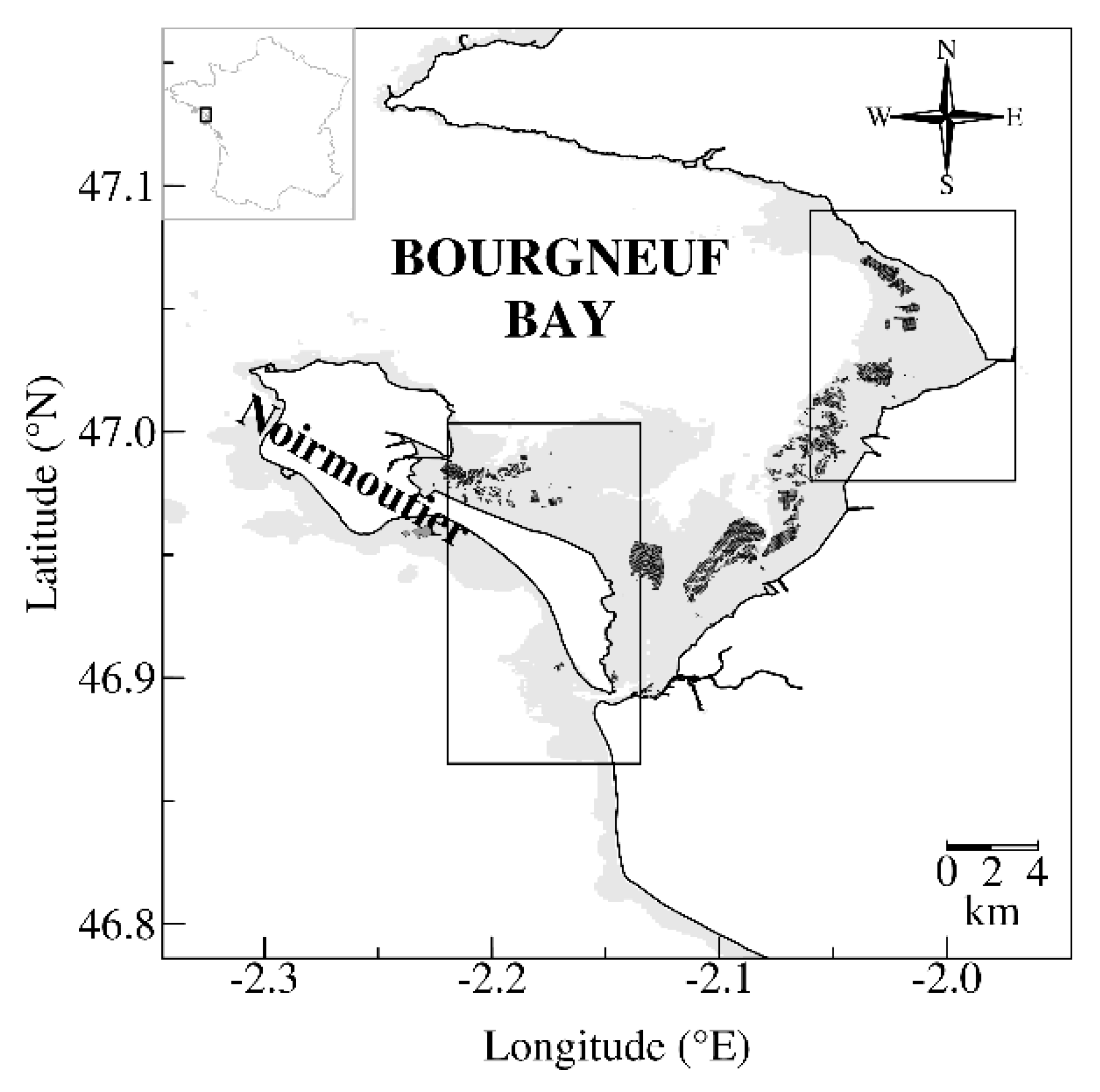
Figure 2.
Comparison between in situ and airborne remote sensing reflectance spectra Rrs(λ) for a variety of reference targets. The airborne data were acquired in Bourgneuf Bay waters, on the 22 September 2009 using HySpex camera. In situ data were acquired using a hyperspectral ASD FieldSpec3 spectrometer. The comparison was performed before reducing the noise by post-processing.

Figure 3.
Example spectra of airborne-derived remote-sensing reflectance, Rrs(λ), at either: the original hyperspectral resolution (a); or the simulated MERIS spectral resolution (b). Pixels were selected to represent the optical diversity generally observed in the northern part of the bay.
Figure 3.
Example spectra of airborne-derived remote-sensing reflectance, Rrs(λ), at either: the original hyperspectral resolution (a); or the simulated MERIS spectral resolution (b). Pixels were selected to represent the optical diversity generally observed in the northern part of the bay.

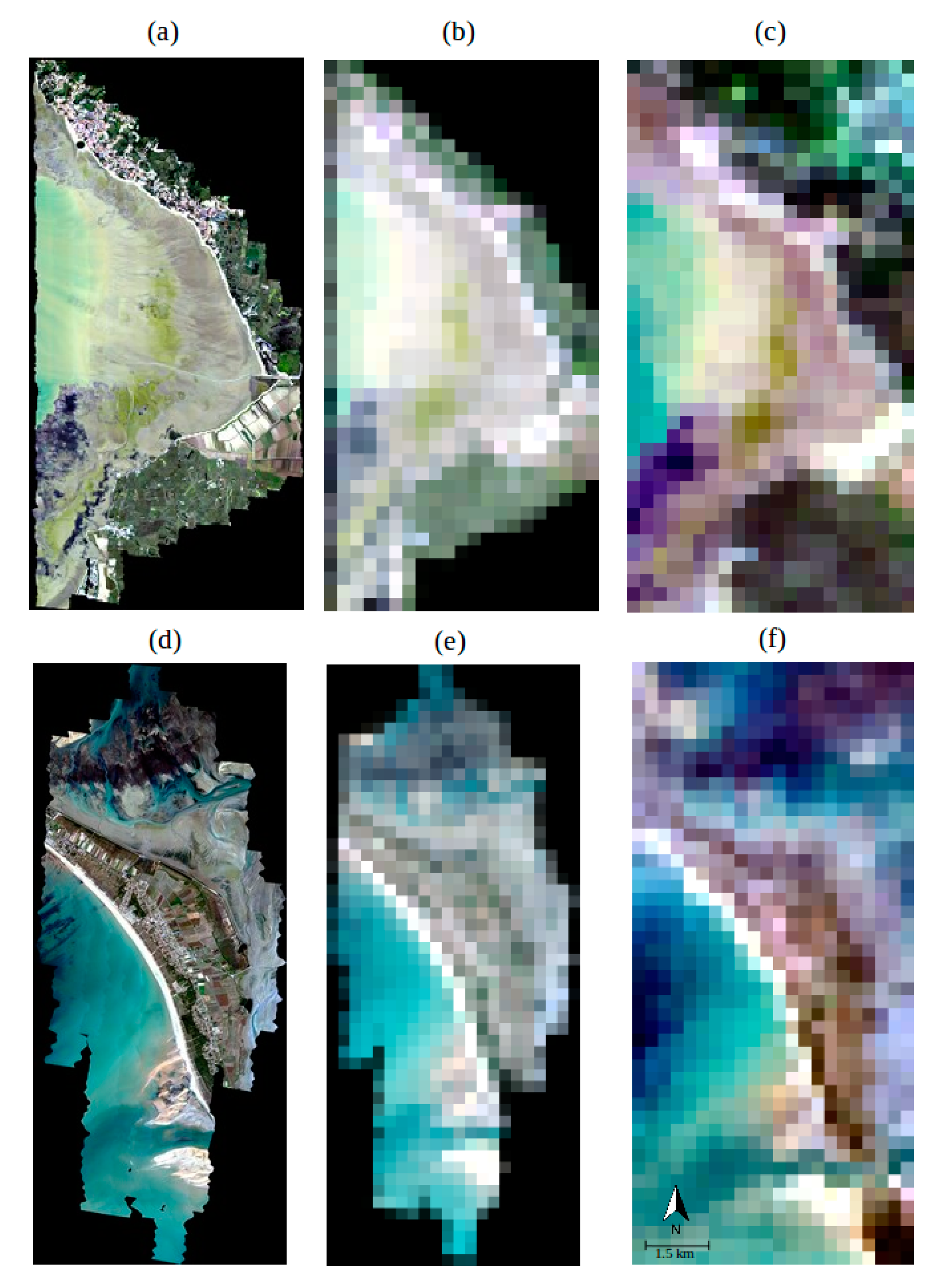
Figure 4.
RGB (red: 620 nm, green: 560 nm, blue: 442.5 nm) images of the two observed sites: Bourgneuf Bay northern mudflat on 28 September 2011 (a–c); and coastal zone off Noirmoutier island on 22 September 2009 (d–f). Airborne data are shown: at their original spatial resolution (1 m) (a,d); and at MERIS-like resolution (300 m) (b,e). Concomitant MERIS images are shown in (c,f).

Figure 5.
For the land pixels: (a) Average spectrum of the ground-truthed airborne remote-sensing reflectance Rrs(λ), in blue line (+/− standard deviation). The corresponding MERIS spectra are shown in black line. (b) Spectral variation of the root mean square error, RMSE(λ), between airborne and MERIS data. Note that the limit of the y-axis was set to that of Figure 6 for comparison purpose.

Figure 6.
For the marine pixels of the three turbidity classes: (a–c) Average spectrum of the ground-truthed airborne remote-sensing reflectance Rrs(λ), in blue line (+/− standard deviation). The corresponding MERIS spectra are shown in green (MEGS), red (SAABIO) and black (FLAASH). (d–f) Similar to (a–c) but for the spectral root mean square error, RMSE(λ), between airborne and MERIS data. The turbidity classes 1, 2, and 3, respectively, correspond to the following ranges of SPM concentration: 0–50, 50–200, and >200 g∙m−3.

Figure 7.
Scatterplot between the concentration of suspended particulate matter (SPM) and the spectrally-averaged root mean square error (RMSE) of: MEGS (a); SAABIO (b); and FLAASH (c) atmospheric corrections for MERIS, using the ground-truthed airborne data as reference.
Figure 7.
Scatterplot between the concentration of suspended particulate matter (SPM) and the spectrally-averaged root mean square error (RMSE) of: MEGS (a); SAABIO (b); and FLAASH (c) atmospheric corrections for MERIS, using the ground-truthed airborne data as reference.

Figure 8.
Comparison between airborne- and MERIS-derived SPM concentration, using: MEGS (a); SAABIO (b); and FLAASH (c) for MERIS atmospheric correction. SPM concentration was computed using a band-switching algorithm [41]. The turbidity classes 1, 2, and 3, respectively, correspond to the following ranges of SPM concentration: 0–50, 50–200, and >200 g∙m−3. The red dashed line corresponds to the 1:1 relationship, and the black dashed line the SPM linear fit, with associated squared coefficient (r2), slope (a), intercept at origin (b), and p-value.

Figure 9.
Examples of intra-pixel variability for three macro-pixels representative of: moderately turbid (a,d,g); highly turbid (b,e,h); and extremely turbid (c,f,i) waters. (a–c) MERIS remote-sensing reflectance Rrs(λ), in black, is compared with the spatially-averaged airborne-derived Rrs(λ), in blue. The blue shade corresponds to the standard deviation of the 90,000 airborne spectra within each macro-pixel. (d–f) Histogram of the 90,000 airborne-derived SPM concentration, represented as a percentage of the mean value. (g–i) Color-scale representation of SPM spatial variation within each macro-pixel.

Figure 10.
For 40 selected macro-pixels, the root mean square error due to MERIS atmospheric correction (RMSEAC, black symbols) or intra-pixel variability (RMSEPIX, grey symbols) is represented as a function of suspended particulate matter (SPM) concentration.
Figure 10.
For 40 selected macro-pixels, the root mean square error due to MERIS atmospheric correction (RMSEAC, black symbols) or intra-pixel variability (RMSEPIX, grey symbols) is represented as a function of suspended particulate matter (SPM) concentration.


Table 1.
Time and date of selected airborne and MERIS images. Low tide time was provided by the national institute for hydrography and oceanography (SHOM). All times are in universal time (UT).
Table 1.
Time and date of selected airborne and MERIS images. Low tide time was provided by the national institute for hydrography and oceanography (SHOM). All times are in universal time (UT).
| Date | Observed Site | Airborne Time | MERIS Time | Low Tide Time 1 |
|---|---|---|---|---|
| 21 September 2009 | northern mudflat | 11:53–13:12 | 11:11 | 11:22 |
| 22 September 2009 | northern mudflat | 10:00–11:19 | 10:40 | 12:03 |
| 22 September 2009 | off Noirmoutier | 11:33–13:13 | 10:40 | 12:24 |
| 28 September 2011 | northern mudflat | 09:59–11:36 | 10:38 | 10:06 |
1 The nearest SHOM stations were used as reference: Pornic for the northern mudflat, and Fromentine off Noirmoutier.
Table 2.
Parameters used in FLAASH for the atmospheric correction of HySpex and MERIS data.
| Parameter | HySpex | MERIS |
|---|---|---|
| Atmosphere visibility | 40 km | 40 km |
| Atmosphere model | US standard | US standard |
| Aerosol model | maritime | maritime |
| Water vapor retrieval | 840 nm | none |
| Aerosol retrieval | none | none |
Table 3.
Number of macro-pixels observed in the land and water classes, after atmospheric correction. For the water pixels, the range of suspended particulate concentration (SPM) concentration in the turbidity classes 1, 2, and 3 is, respectively, 0–50, 50–200, and > 200 g∙m−3.
Table 3.
Number of macro-pixels observed in the land and water classes, after atmospheric correction. For the water pixels, the range of suspended particulate concentration (SPM) concentration in the turbidity classes 1, 2, and 3 is, respectively, 0–50, 50–200, and > 200 g∙m−3.
| Pixel Type | HySpex | MERIS-MEGS | MERIS-SAABIO | MERIS-FLAASH |
|---|---|---|---|---|
| Land | 426 | NA | NA | 426 |
| Water (all classes) | 398 | 385 | 385 | 398 |
| Water (class 1) | 166 | 163 | 163 | 166 |
| Water (class 2) | 104 | 103 | 103 | 104 |
| Water (class 3) | 128 | 119 | 119 | 128 |
Table 4.
Averaged root mean square error (RMSE) and relative RMSE between airborne reference and MERIS Rrs(λ) retrieved using either the MEGS, SAABIO or FLAASH atmospheric correction. The RMSE and RRMSE are indicated for the land and water pixels, and for each turbidity class. Turbidity classes 1, 2, and 3, respectively, correspond to SPM ranges: 0–50, 50–200, and >200 g∙m−3.
| Pixel Type | Metrics 1 | MEGS | SAABIO | FLAASH |
|---|---|---|---|---|
| Land | RMSE | NA | NA | 0.0035 |
| RRMSE | NA | NA | 14 | |
| Water (all) | RMSE | 0.0104 | 0.0137 | 0.0039 |
| RRMSE | 53 | 70 | 45 | |
| Water (class 1) | RMSE | 0.0058 | 0.0041 | 0.0045 |
| RRMSE | 53 | 49 | 81 | |
| Water (class 2) | RMSE | 0.0152 | 0.0128 | 0.0028 |
| RRMSE | 64 | 58 | 22 | |
| Water (class 3) | RMSE | 0.0127 | 0.0274 | 0.0041 |
| RRMSE | 46 | 108 | 16 |
1 RMSE is in sr−1, and RRMSE in %.
© 2018 by the authors. Licensee MDPI, Basel, Switzerland. This article is an open access article distributed under the terms and conditions of the Creative Commons Attribution (CC BY) license (http://creativecommons.org/licenses/by/4.0/).
Share and Cite
MDPI and ACS Style
Larnicol, M.; Launeau, P.; Gernez, P. Using High-Resolution Airborne Data to Evaluate MERIS Atmospheric Correction and Intra-Pixel Variability in Nearshore Turbid Waters. Remote Sens. 2018, 10, 274. https://doi.org/10.3390/rs10020274
AMA Style
Larnicol M, Launeau P, Gernez P. Using High-Resolution Airborne Data to Evaluate MERIS Atmospheric Correction and Intra-Pixel Variability in Nearshore Turbid Waters. Remote Sensing. 2018; 10(2):274. https://doi.org/10.3390/rs10020274
Chicago/Turabian StyleLarnicol, Morgane, Patrick Launeau, and Pierre Gernez. 2018. "Using High-Resolution Airborne Data to Evaluate MERIS Atmospheric Correction and Intra-Pixel Variability in Nearshore Turbid Waters" Remote Sensing 10, no. 2: 274. https://doi.org/10.3390/rs10020274
Note that from the first issue of 2016, this journal uses article numbers instead of page numbers. See further details here.