A Semi-Empirical SNR Model for Soil Moisture Retrieval Using GNSS SNR Data

1
School of Electronic and Information Engineering, Beihang University, Beijing 100191, China
2
Beijing Vegetable Research Center, Beijing Academy of Agricultural and Forestry Sciences, Beijing 100097, China
*
Author to whom correspondence should be addressed.
Remote Sens. 2018, 10(2), 280; https://doi.org/10.3390/rs10020280
Submission received: 26 November 2017
/
Revised: 8 February 2018
/
Accepted: 9 February 2018
/
Published: 11 February 2018
(This article belongs to the Special Issue Soil Moisture Remote Sensing Across Scales)
Abstract
:The Global Navigation Satellite System-Interferometry and Reflectometry (GNSS-IR) technique on soil moisture remote sensing was studied. A semi-empirical Signal-to-Noise Ratio (SNR) model was proposed as a curve-fitting model for SNR data routinely collected by a GNSS receiver. This model aims at reconstructing the direct and reflected signal from SNR data and at the same time extracting frequency and phase information that is affected by soil moisture as proposed by K. M. Larson et al. This is achieved empirically through approximating the direct and reflected signal by a second-order and fourth-order polynomial, respectively, based on the well-established SNR model. Compared with other models (K. M. Larson et al., T. Yang et al.), this model can improve the Quality of Fit (QoF) with little prior knowledge needed and can allow soil permittivity to be estimated from the reconstructed signals. In developing this model, we showed how noise affects the receiver SNR estimation and thus the model performance through simulations under the bare soil assumption. Results showed that the reconstructed signals with a grazing angle of 5°–15° were better for soil moisture retrieval. The QoF was improved by around 45%, which resulted in better estimation of the frequency and phase information. However, we found that the improvement on phase estimation could be neglected. Experimental data collected at Lamasquère, France, were also used to validate the proposed model. The results were compared with the simulation and previous works. It was found that the model could ensure good fitting quality even in the case of irregular SNR variation. Additionally, the soil moisture calculated from the reconstructed signals was about 15% closer in relation to the ground truth measurements. A deeper insight into the Larson model and the proposed model was given at this stage, which formed a possible explanation of this fact. Furthermore, frequency and phase information extracted using this model were also studied for their capability to monitor soil moisture variation. Finally, phenomena such as retrieval ambiguity and error sensitivity were stated and discussed.
1. Introduction
Soil Moisture Content (SMC) is a key parameter in the study of agriculture and the global water cycle. The Time-Domain Reflectometer (TDR), Frequency-Domain Reflectometer (FDR) and active/passive remote sensing methods [1] have been developed to measure SMC. In 1993, Martín-Neira proposed an ocean altimetry system called the Passive Reflectometry and Interferometry System (PARIS), which uses Global Positioning System (GPS) reflected signals. Later, researchers demonstrated its feasibility on soil moisture measurement from different platforms including ground-based [2], airborne [3,4] and space-borne [5]. These studies use specially-designed receivers equipped with two antennas of different polarizations (right-handed circularly polarized and left-handed circularly polarized) to collect the direct and reflected signals, respectively [6]. All the results demonstrate that the L-band navigation signals are very sensitive to SMC, which is in accordance with microwave remote sensing theory (F. T. Ulaby et al., 2013 [7]).
In recent years, parallel studies have shown that continuously operating GNSS receivers with one geodetic-quality antenna can also be used to sense environmental parameters including soil moisture [8], snow depth [9] and tides [10]. This technique is called the Interference Pattern Technique (IPT) or Global Navigation Satellite System Interferometry and Reflectometry (GNSS-IR). It focuses on studying the temporal changes of SNR data that are affected by reflected signals that in turn are affected by the environment surrounding the antenna. Among these applications, soil moisture monitoring has gained wide interest. Part of the efforts made in this field is to extract SMC-related metrics from SNR data and develop models to retrieve SMC. K. M. Larson et al. performed a series of analyses on SNR data collected by receivers that are affiliated with the the EarthScope Plate Boundary Observatory (PBO) [8]. Additionally, three metrics were extracted from SNR including amplitude, phase and frequency (reflector height) using the SNR model proposed by K. M. Larson et al. [11] (hereafter referred to as the Larson model). Results showed that these metrics were empirically in linear relation to in situ soil moisture. Several scenario-dependent empirical models have been developed to retrieve SMC based on this observation [12,13]. Besides using the geodetic-quality antenna that is Right-Handed Circularly Polarized (RHCP), other researchers proposed using linearly-polarized antennas to collect the SNR data. In these cases, the characteristics of SNR variation are different from the previous one; thus, new metrics have been discovered such as “notch” [14] and the “local minima and maxima” [15,16] of SNR. Results showed that it was possible to estimate the soil permittivity from these new metrics, after which well-developed dielectric models on microwave frequencies can be used to retrieve soil moisture (M. T. Hallikainen et al. 1985 [17], J. R. Wang et al. 1980 [18]). However, since the use of linearly-polarized antenna changes the normal hardware configuration of GNSS receivers, this may prevent its wide usage.
Recent efforts made by T. Yang et al. [19] showed that it was also possible to extract soil permittivity from SNR data collected via an RHCP antenna. This was achieved by incorporating soil permittivity into well-established SNR model (V. U. Zavorotny et al. 2010 [20]) and fitting with SNR data directly using the Least SQuare(LSQ) method. As seen from the results, the Quality of Fit (QoF) could be improved compared with the Larson model, which used a polynomial de-trending followed by cosine modeling. However, this cannot be achieved if the scattering mechanism and system parameters such as the antenna gain pattern are unknown in advance.
In this paper, a semi-empirical SNR model was proposed as a curve-fitting model. It aimed at reconstructing the direct and reflected signals from SNR data collected via one RHCP antenna and simultaneously extracting frequency and phase metrics related to SMC. Compared with previous models, the QoF could be improved with little prior knowledge needed, and the estimation accuracy of frequency and phase was better. We demonstrated that it was also possible to estimate soil permittivity from the reconstructed signals through necessary corrections such as the antenna gain pattern. The model design was also based on the well-established SNR model, but we empirically chose a second-order and fourth-order polynomial to approximate the direct and reflected signal, respectively. The justification for introducing the high-order polynomial is that it is easier to model high-order attenuation experienced by the reflected signals in reality. In developing this model, we showed how noise affects the receiver SNR estimation and thus the model performance through simulation under the bare soil assumption, which was seldom considered in the previous simulation studies of this field. Furthermore, experimental data collected at Lamasquère, France [21], were also used to validate the proposed model. The results were evaluated and compared with previous works. A deeper insight into the Larson model was given at the same time, and the reason why it cannot give good results was clearly explained.
This paper is organized as follows. Section 2 re-examines the SNR model from the receiver’s point of view, which lays the foundation for the subsequent model design and simulation. Section 3 describes the design and application of the proposed model in detail. In Section 4, the simulation settings are described. The model performance is analyzed under the effect of noise. In Section 5, experimental data validation is performed. The results are given and compared with simulations and previous works. Section 6 discusses the problems and phenomena that appeared in the simulation and experimental data validation. Finally, Section 7 summarizes the main conclusions of this paper.
2. Receiver SNR Modeling and Estimation under Noise
The GNSS-IR technique utilizes the interference phenomenon that occurs between the direct signal and the ground multipath/reflected signal. Although this phenomenon happens spontaneously at the front of the antenna regardless of receiver architecture, it cannot be easily observed because of the spread spectrum technology used in the navigation signal. Normally, the power of the spread spectrum signal is lower than the noise power, which causes the interference effect to be embedded in noise. Hence, a de-spread operation, which is implemented as a correlator, is commonly performed within the GNSS receiver [22] to increase the SNR. Therefore, the interference effect can be detected. The result of this operation can be described by the well-established receiver signal model. Under the assumption of perfect carrier frequency tracking in a GPS receiver, the baseband signal from the correlator output can be expressed as [23]:
where is the transmitted carrier power, is the normalized auto-correlation function of the PRN (Pseudo-Random Noise) modulation code, is narrow band complex white Gaussian noise with identical independent distribution in its real and imaginary part, and are the local code and carrier phase, respectively, is the attenuation factor and and are the code and carrier phase delay of the incoming signal, respectively, with representing the direct signal. Note that , and are all functions of satellite elevation angle, which in turn is a function of time implicitly; K is the total number of multipath signals. In subsequent descriptions, K is assumed to be one. This assumption is reasonable if the antenna height is low and the ground is flat (surface height variation is less than one wavelength). Navigation bit modulation is assumed to be known in advance through methods such as external aiding [23], and thus, long-time coherent accumulation is allowed to improve SNR estimation.
According to [23], the SNR of the base-band GNSS signal can be expressed as follows:
In signal estimation theory, the Maximum Likelihood Estimate (MLE) is a method that can be used to estimate the SNR. Let = be a vector of M consecutive correlator output in the period of T seconds, where M is given by and is the modulation code period. is assumed to be 1 ms hereafter. In the ground-based case, when T is less than 1 s, the multipath variation is slow, so all the entries of vector can be assumed equal if no noise is presented.
Finally, SNR is estimated as:
M can be seen as the number of coherent accumulations, and it determines how noisy the SNR estimation is. As M increases, the noise on SNR data decreases.
Also note that the numerator of Equation (3) is the maximum likelihood estimation of . Since is approximately zero in the ground-based case, and thus , then after some manipulation, the following equation can be obtained:
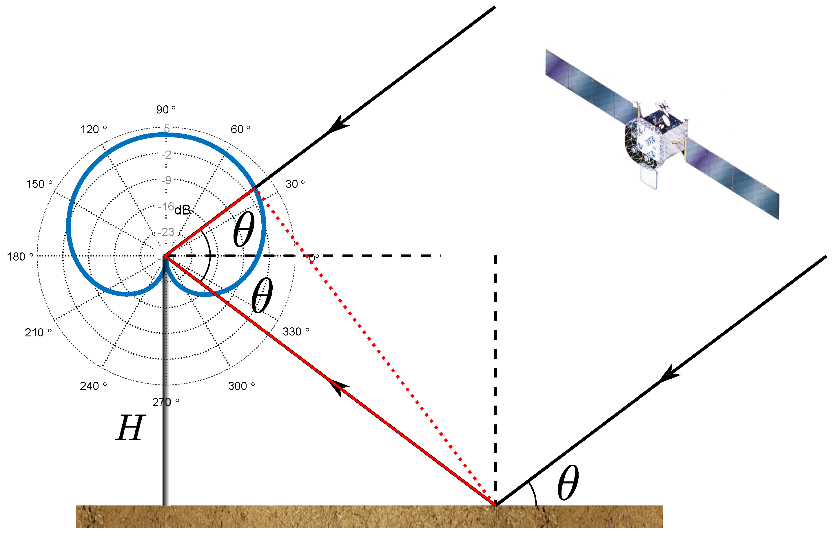
where contains the phase of the attenuation and additional phase terms, the local carrier phase in Equation (1) is canceled during manipulation and is the phase difference between the direct and reflected signal caused by the path difference (see Figure 1) that can be modeled as:
where is the wavelength, is satellite elevation angle and H is antenna effective height [20], which determines the frequency of SNR variation. In general, Equation (4) is a commonly-used SNR model assuming only specular reflection. Typical multipath reflection geometry is illustrated in Figure 1.
3. Semi-Empirical SNR Model: SNR Metrics’ Retrieval
In Equation (4), and are inherited from Equation (1) to account for various nonlinear attenuation factors in the signal transmitting, propagating and processing chain. In the ground-based case, some of these factors are nearly the same for direct and reflected signals, including the effect of satellite antenna gain pattern, atmosphere [24], Radio Frequency (RF) front-end devices (for example, Automatic Gain Control (AGC) [25]), etc. However, significant differences appear when it comes to receiver antenna gain and scattering loss. Firstly, in a normal geodetic receiver configuration, antenna gain is designed to decay rapidly at the bottom to suppress the multipath signal, so the attenuation is more severe on the reflected signal than on the direct signal. Secondly, the reflected signal suffers from additional loss caused by land scattering, which is governed by electromagnetic theory. When only specular reflection and the RHCP signal component are considered, the scattering can be described by the RR (RHCP to RHCP) reflection coefficient [26]:
where is satellite elevation angle and is soil relative permittivity.
It can be concluded that the reflected signal experiences higher order variation than the direct signal. Therefore, a high-order polynomial is proposed to approximate the decibel attenuation of the reflected signal, while a low-order polynomial is used to approximate the decibel attenuation of the direct signal. The idea can be expressed as:
where is the polynomial function, and represent the order of the corresponding polynomial and . The minus sign in Equation (7b) indicates that the reflected signal is incident from the bottom of the antenna as shown in Figure 1.
By substituting Equation (7) into Equation (4), the new SNR model can be obtained as follows:
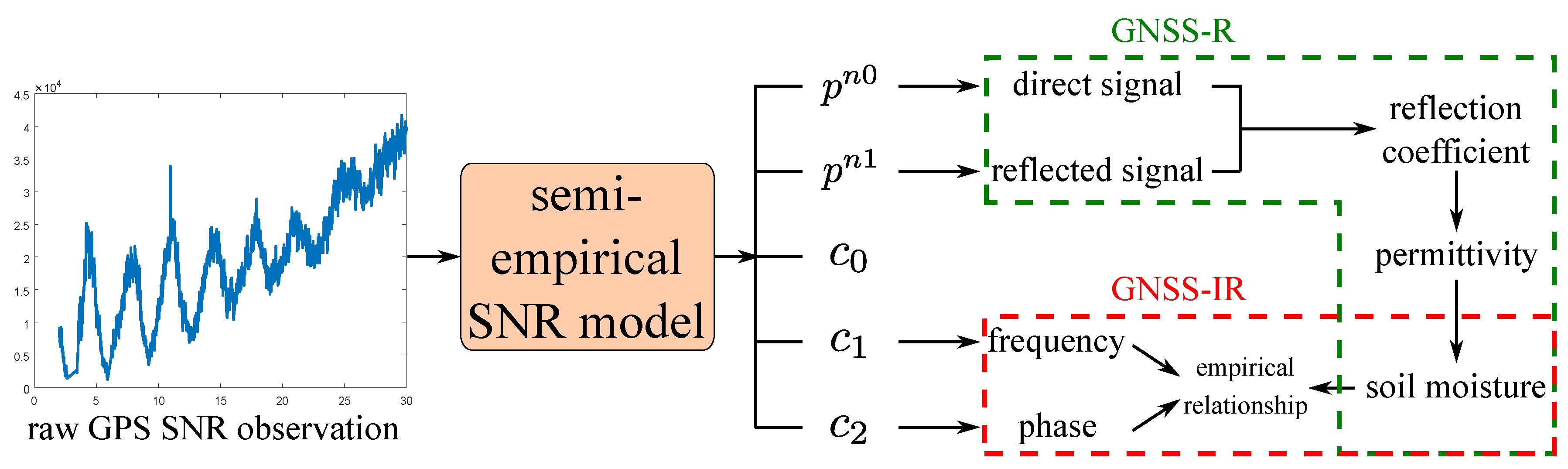
where represents the SNR offset (when expressed in a base-10 logarithm) and , represent the frequency and phase of interference pattern, respectively. Taking the coefficients of these polynomials into account, there are undetermined parameters in total. All of them can be obtained by fitting Equation (8) with the low-elevation-angle SNR observation. Subsequent retrieval can be performed using two existing methods. Firstly, two polynomials representing direct and reflected signals can be used to estimate the reflection coefficient, which is mainly determined by soil moisture. In this procedure, common attenuation factors contained in the reconstructed signals can be partially canceled. This is similar to the GNSS Reflectometry (GNSS-R) method except that co-polarization is used rather than cross-polarization. Secondly, estimated phase and frequency can also be used to study how they are related to soil moisture empirically. The overall retrieval procedure is illustrated in Figure 2.
The remainder of this paper is dedicated to the study of the performance of this SNR model through simulation and experimental data validation.
4. Simulations
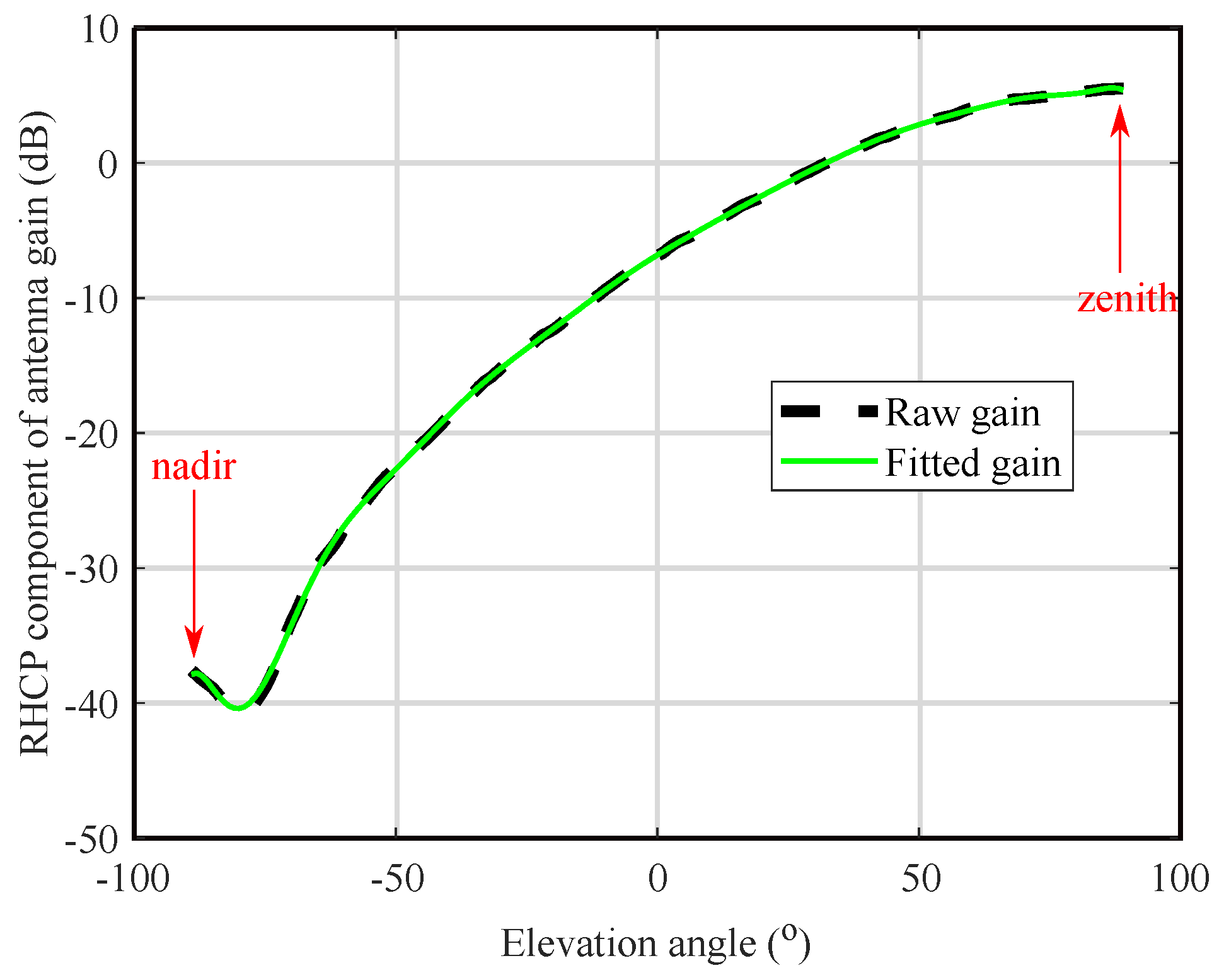
In this section, SNR data were generated considering noise, the reflection coefficient and the receiver antenna gain pattern as the main factors mentioned in Section 2 and Section 3. Additionally, the model validation was based on the simulated SNR. Among these factors, the antenna gain pattern used is shown in Figure 3, which is a measurement of the RHCP component of one actual antenna [21]. An eighth-order Fourier fitting was used to smooth the gain pattern. It was assumed that the antenna gain was omnidirectional.
Table 1 shows other simulation parameters used.
In Table 1, single sideband power spectrum density and front-end bandwidth B were used to calculate base-band noise variance. The simulated noise made it possible to investigate the model performance statistically under different noise conditions. This was achieved by varying the number of coherent accumulation M. If necessary, the simulation was performed 200 times for each M value to cover different realizations of this stochastic process. Finally, Hallikainen’s well-known empirical dielectric model [17] was used to simulate the soil moisture’s effect on reflected signal through relative permittivity . Under the assumption that the soil type is silt clay that contains 18% sand (S) and 41% clay (C) in terms of textural components (measured by weight) [21] and has zero conductivity, the empirical model can be expressed as follows:
4.1. Simulation Results: Reconstruction and Retrieval
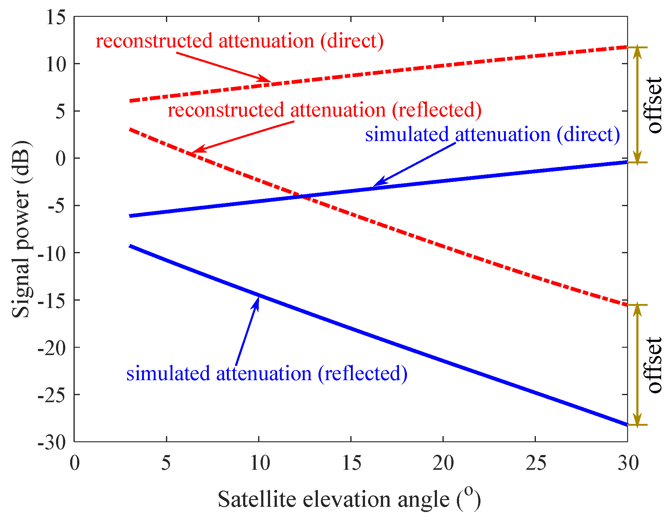
To test the behavior of this SNR model under weak noise conditions, the number of coherent summation M was set to 400 ms temporarily, in which case the noise variance is relatively small. The reconstructed signals after fitting are shown in Figure 4.
The results shown in Figure 4 were obtained with a QoF of about 0.95. The QoF was calculated as follows:
where is raw data and represents the fitting result.
Figure 4 shows that reconstructed signals varied nearly the same as the simulated signals, but had an offset. This means that the proposed semi-empirical model could not be used to reconstruct the signal absolutely. This offset was the difference between estimated offset and the true value of , where is noise variance. Since the offset is nearly the same for both the direct and reflected signal, it can be canceled in the subsequent processing. Then, according to bistatic radar Equation [25] and considering only specular reflection, the reflectivity can be expressed as:
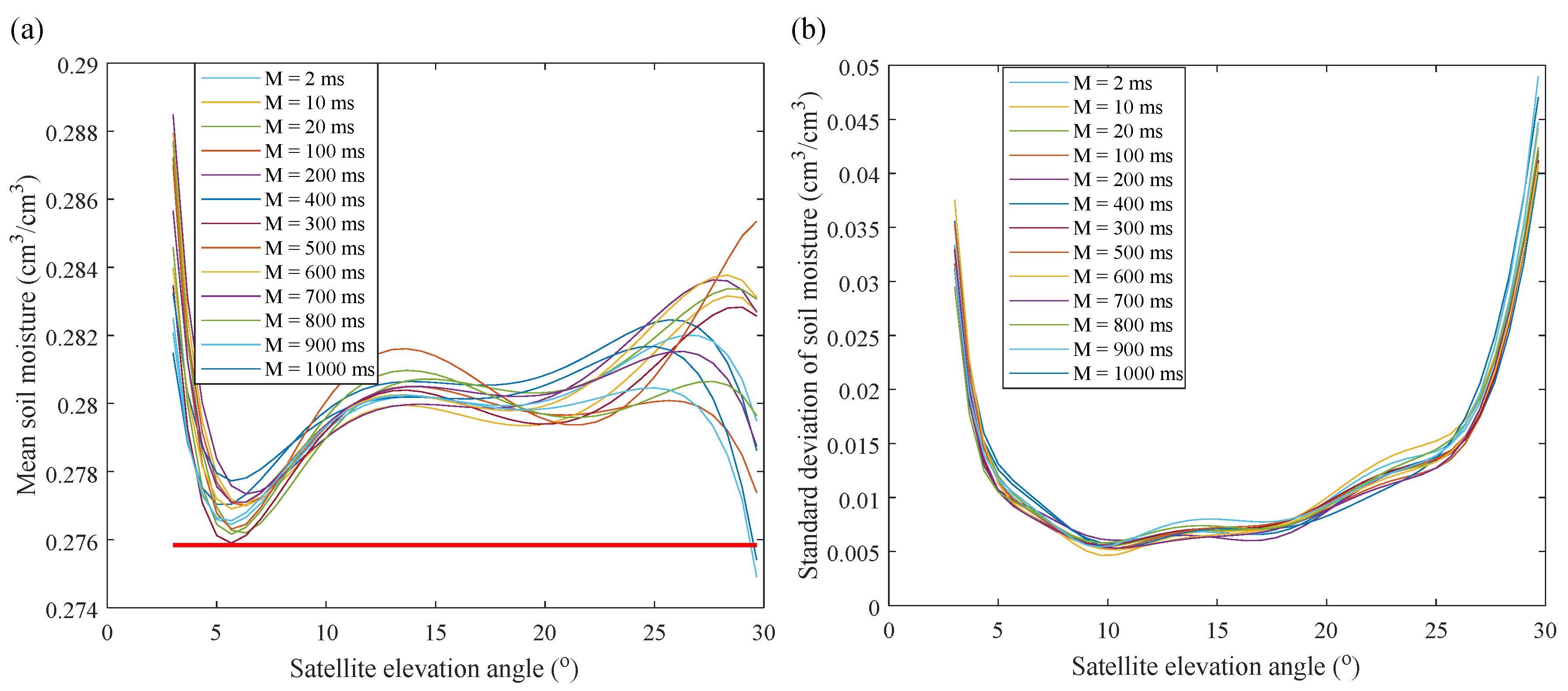
where and are antenna gain experienced by the direct and reflected signal, respectively. They were recorded in [21] and are shown in Figure 3. Then, soil moisture can be calculated using Equations (6) and (9). Figure 5 shows statistical results obtained from 200 simulations for each M value. In Figure 5a, the bold red line represents the true soil moisture, which was used to generate the SNR. It shows that the mean retrieval results deviated from the true value under all the elevation angles. The maximum deviation was about 0.01 , which appeared at 3°. Also note that the variation of mean retrieval results was similar to the variation of the fourth-order polynomial, which was caused by the SNR model used. Figure 5b shows that the standard deviation of SMC retrieval varied from 0.005 to 0.05 . A large standard deviation appeared at both ends. Then, it can be concluded that the reflected signal with a 5°–15° grazing angle is more suitable for performing retrieval.
4.2. Simulation Results: Phase and Frequency Estimation
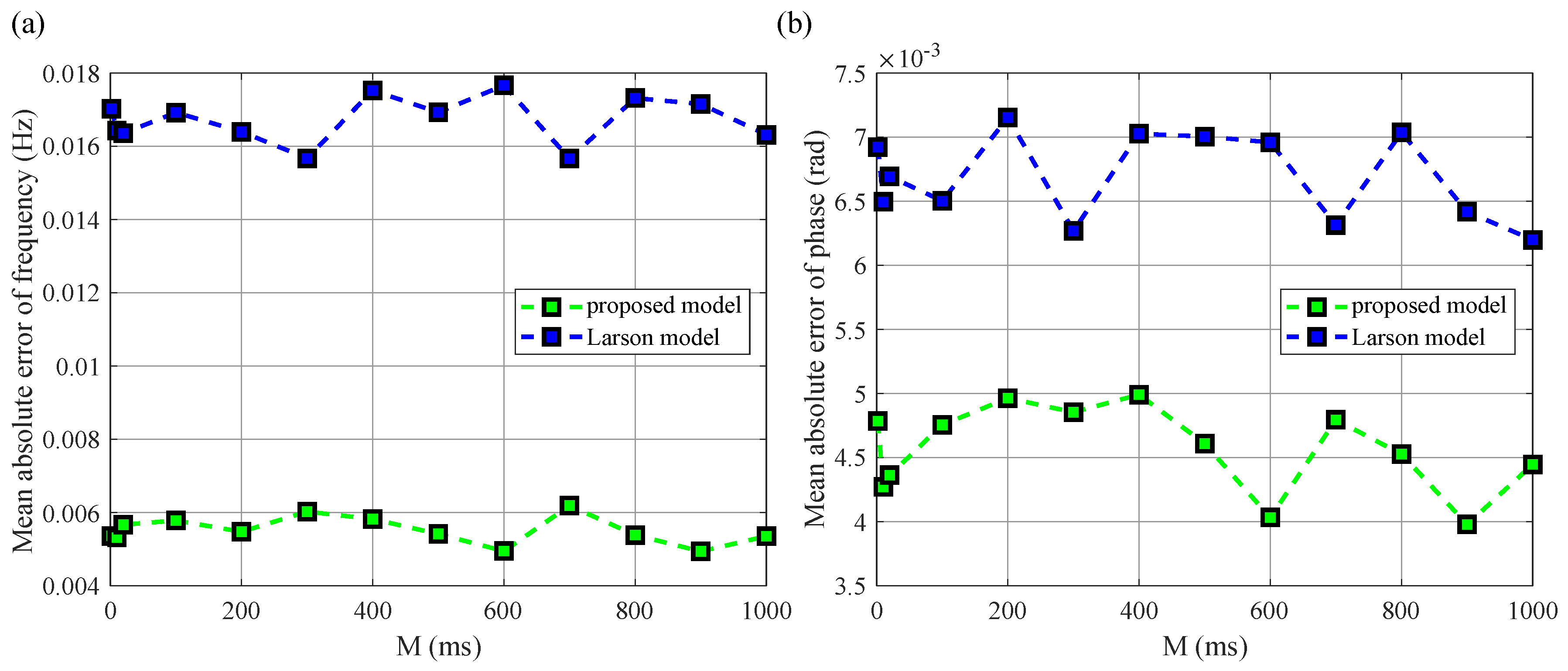
Phase and frequency estimation results were compared with those obtained using the Larson model and are shown in Figure 6.
Figure 6 shows that the estimation error is reduced under all the noise conditions (indicated by the change of M) for both of the metrics. It can also be seen that the noise on SNR data does not significantly affect the estimation error either of the metrics, which might indicate that the pre-processing of SNR data such as filtering would not improve estimation error significantly. Furthermore, it is necessary to compare the extent to which the estimation accuracy is improved. The improvement is calculated as follows:
where represents errors obtained from the proposed model, represents errors obtained from the Larson model, represents the true value of the SNR metric and represents the number of M values, which is 13 in this simulation. Results showed that the accuracy improvement in frequency estimation was 0.0214, while the improvement in phase estimation was only 1.0113 × 10, which could be neglected compared with the frequency estimation. Actually, all the improvements were motivated by the improved QoF values (from 0.55 to 0.95), which were achieved by the proposed SNR model.
5. Experimental Data Validation
To validate the simulation results, GPS L1 data collected at Lamasquère, France (43°29′14.45″N; 1°13′44.11″E), were processed, covering about 40 days from 5th of February 2014 to 15th of March 2014 [21]. The site was a soya field equipped with a Leica GR25 receiver and an AR10 antenna. At the same time, a Theta Probe ML3 soil moisture sensor was installed to collect ground truth measurements. The sensor measured soil moisture every 2 min at 2-cm and 5-cm depths and was located a few meters away from the receiver. The antenna height was about 1.7 m. The soil type is silt clay, which consists of 18% sand, 41% clay and 41% silt. The soil temperature variation was between 5 °C and 16 °C. Additionally, the ground was nearly bare in the entire experiment period. Other site information is thoroughly recorded in [21], so its description is omitted here. Since the proposed SNR model tries to reconstruct the reflected signal, only the low-elevation-angle (2−30) SNR with strong reflection was processed.
5.1. Soil Moisture Retrieval Using the Reconstructed Signal
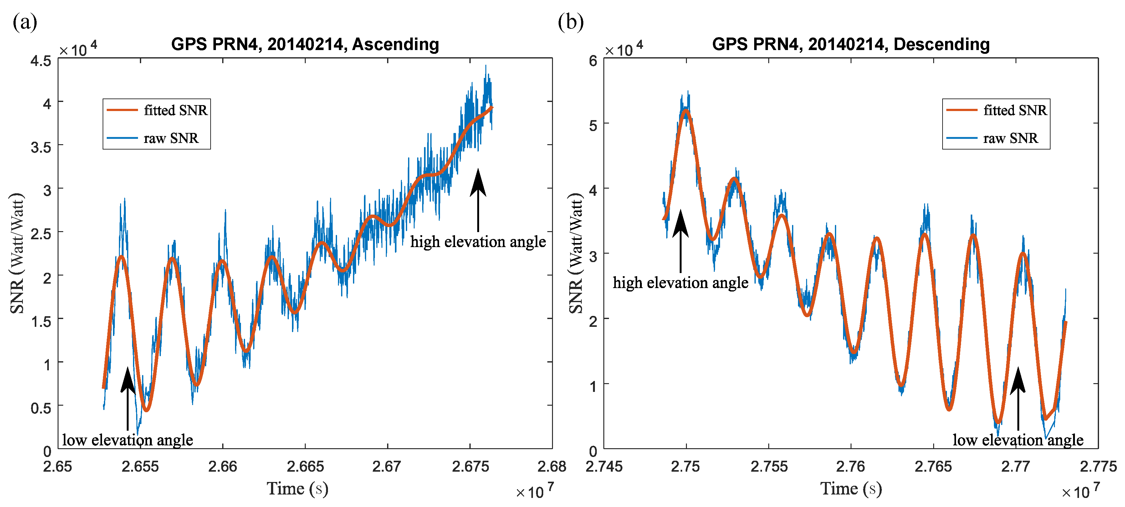
Firstly, the actual fitting results of the ascending path and descending path are shown in Figure 7 using GPS PRN No. 4 as an example. The orders of polynomials were the same as those used in the simulation.
The QoF values for the ascending and descending path were 0.9123 and 0.9392, respectively. Normally, the SNR fluctuation becomes weaker at a higher elevation angle according to the simulation, which should also look like the ascending path shown in Figure 7a. However, the SNR of the descending path showed some irregular variation: (1) the oscillation amplitude suddenly increased at a high elevation angle; and (2) the amplitude attenuation rate was slow compared with the ascending path. This means that some additional sources of high-order variation experienced by the reflected signal may not have been covered in the simulation. However, as seen from Figure 7b, the fourth-order polynomial used in the proposed SNR model could track the irregular variation adequately.
Secondly, soil moisture retrieval was carried out following the procedure described in Section 4.1 and Figure 2. However, Equation (11) should be modified to take soil roughness [27] into consideration by introducing a correction term:
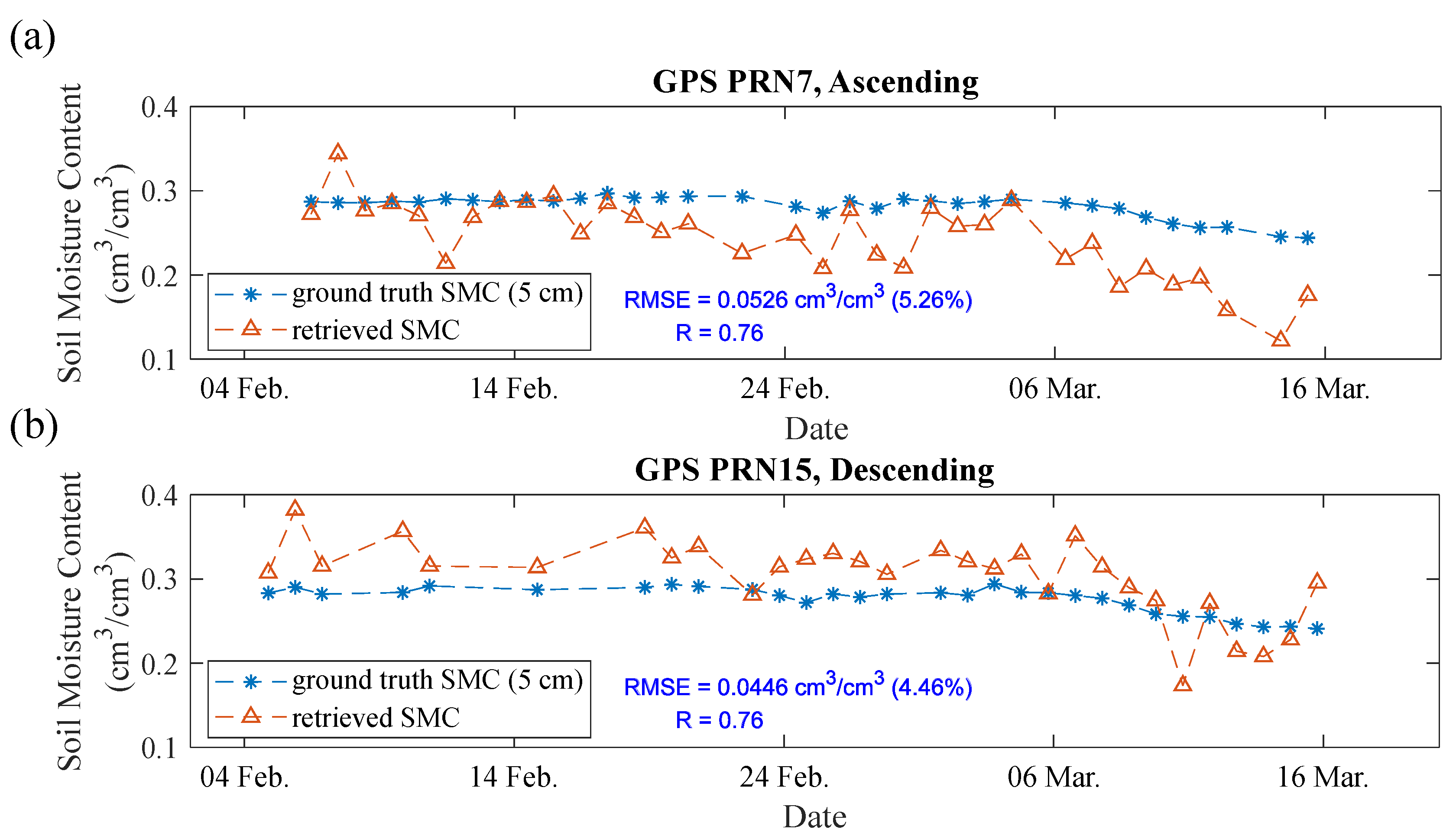
where is mean surface height variation, which was assumed to be 2 cm here. According to the simulation results obtained in Section 4.1, retrieval results between 5° and 15° were both accurate and relatively stable. Here, the 10° elevation angle was chosen to perform retrieval. This indicated that the specular point would be located at about 10 m from the receiver, and the first Fresnel zone covered an area of about 39 . This setting was the same for all the satellites. The retrieval results given by the descending and ascending path were compared with ground truth measurements separately. The results with the best Root-Mean-Square Error (RMSE) are shown in Figure 8.
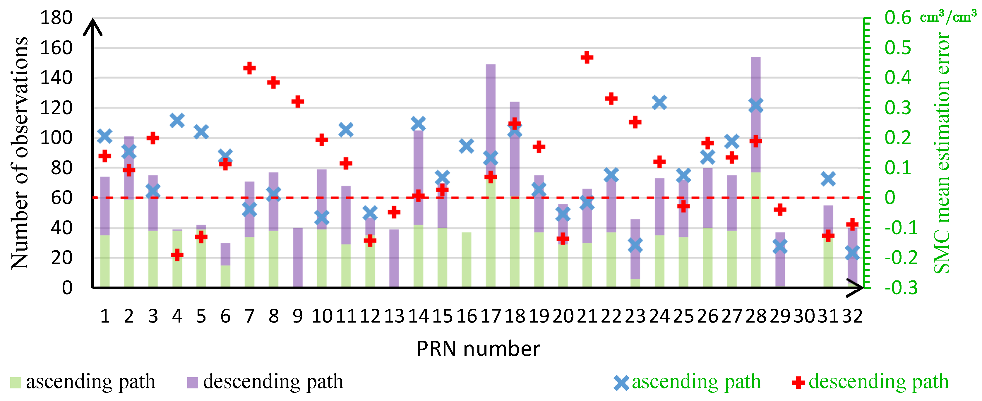
Figure 8a shows the time series of retrieved SMC during satellite PRN No. 7’s ascending period. The RMSE was 0.0526 , and the correlation coefficient R was 0.76. As for the descending period, PRN No. 15 gave the best results, with an RMSE of 0.0446 and a correlation coefficient R of 0.76. Note that a few missing points shown in Figure 8 were retrieval results that fell out of the range 0.06−0.99 . These points were considered as bad data points. The choice of this criterion will be discussed in Section 6.2. By contrast, almost all of the retrieval results given by the descending path of PRN No. 4 fell outside of this range, as shown in the bar plot in Figure 9. This was caused by the irregular SNR variation shown in Figure 7b. Thus, although the proposed SNR model is able to track the irregular variation, a large SMC retrieval error will still occur if subsequent processing cannot find out the causes and correct their effects.
In Figure 9, the bar plot with the y-axis on the left shows the number of valid retrieval results belonging to each satellite’s ascending and descending path during the 40 days of observations. The scatter plot with the y-axis on the right shows the Mean Error (ME) calculated as the mean difference between the retrieved SMC values and the ground truth measurements. Positive ME indicates that the retrieved SMC values were generally greater than ground truth measurement values during the entire experiment period. As a whole, more than 70% of the satellites gave larger retrieval values than ground truth values for both the ascending and descending path. This phenomenon might validate one of the simulation results shown in Figure 5a, where the mean retrieval values were larger than the true values at a 10° elevation angle. Also note from Figure 9 that the mean errors showed some repeating patterns in terms of PRN number, for example the descending path MEs of PRN Nos. 7 to 11 and PRN Nos. 21 to 25. This was caused by a similar reflection geometry formed between the antenna and the two groups of satellites, which was indicated by similar satellite elevation angles (2°−30°) and azimuth angle range (for PRN Nos. 7 to 11, it was 59°−149°, and for PRN Nos. 21 to 25, it was 64°−128°).
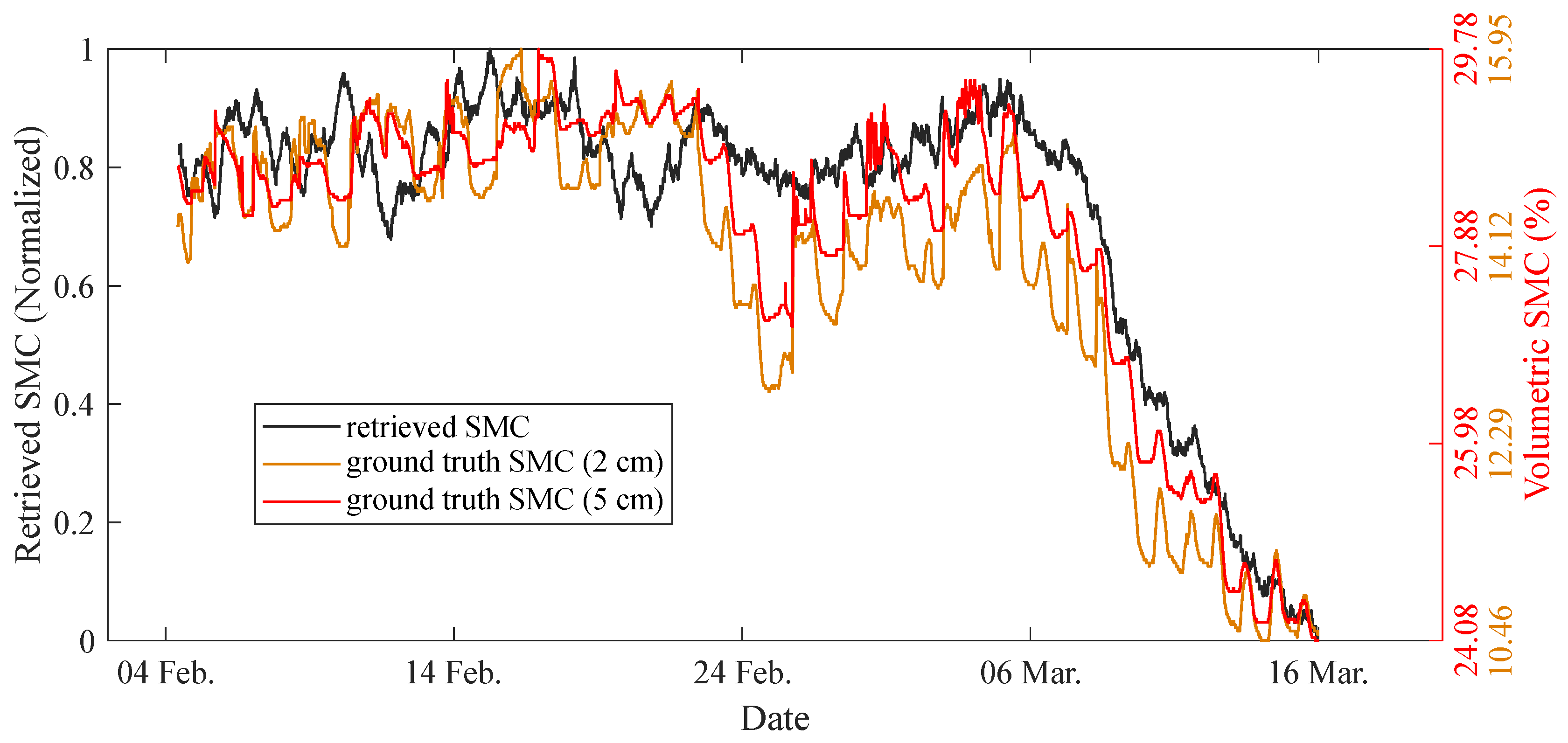
Next, in order to facilitate further comparison and to increase the time resolution, the method proposed by N. Roussel et al. [21] was used. The ground truth measurements and retrieval results obtained from both the ascending and descending path of different satellite were normalized to 0−1 and then combined into a time series. After that, a moving average was performed to smooth the time series with a moving window specified by step length and half window width . In this and subsequent processing, was set to 10 min, which was the same as in [21]. The correlations between ground truth measurements and combined retrieval results are shown in Figure 10.
In this processing, 22.13% bad data points whose retrieval results fell out of range 0.06−0.99 were discarded before normalization and smoothing. The remaining points were smoothed with a half window width . The resulting correlation coefficient R with 5-cm SMC was 0.9370, while the correlation coefficient with 2-cm SMC was 0.8824. Both of the results were obviously improved compared with the correlation coefficient (, , 2-cm SMC) obtained using the amplitude metric as presented in [21]. Note that a reduced window width still resulted in a large improvement in R. Similar results were also shown by C. Chew et al. [12] that the correlation between amplitude and SMC was low compared with that obtained from the other two metrics. The reason why the amplitude obtained from the Larson model did not give good results was mainly caused by de-trending of raw SNR through polynomial fitting directly. It was previously thought that the de-trended signal could be normally expressed by a cosine function:
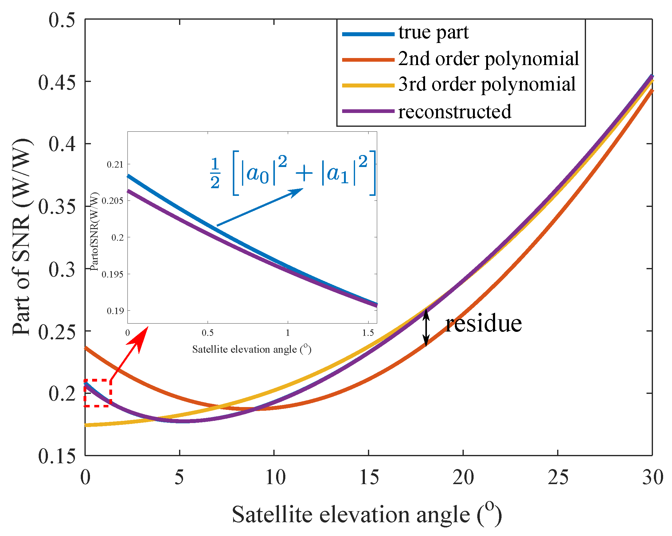
The form of Equation (14) is exactly the same as the third term in Equation (4). This means that this term can only be obtained if we can model adequately and subtract it from Equation (4). However, simulation results showed that polynomial fitting of raw SNR failed to model the direct and reflected signal components and thus failed to model the interference effect. This is shown in Figure 11. In Figure 11, all of the signals were normalized by the carrier power to facilitate comparison. The difference between the true part of SNR and polynomial fitting of raw SNR was more obvious at a low elevation angle. As a result, the residue of the direct and reflected signal enters the de-trended signal, which is an additive effect. In addition, the direct signal also couples with a reflected signal in the amplitude of the de-trended signal according to Equation (4), which is a multiplicative effect. Hence, all the factors that contribute to direct and reflected signal variation will also impact the amplitude estimation. The difficulty in estimating the direct signal also caused a difficulty in correcting the amplitude estimation. To conclude, the amplitude extracted from the Larson model is a rough representation of reflected signal variation. From another point of view, the reflection coefficient can be seen as a refined version of multipath amplitude, which truly represents soil moisture variation. The essence of the proposed SNR model is to reconstruct the reflection coefficient through decoupling/reconstructing the direct and reflected signal. In this sense, the proposed SNR model could be expected to give better results.
5.2. Correlation between SMC and Frequency/Phase Estimation
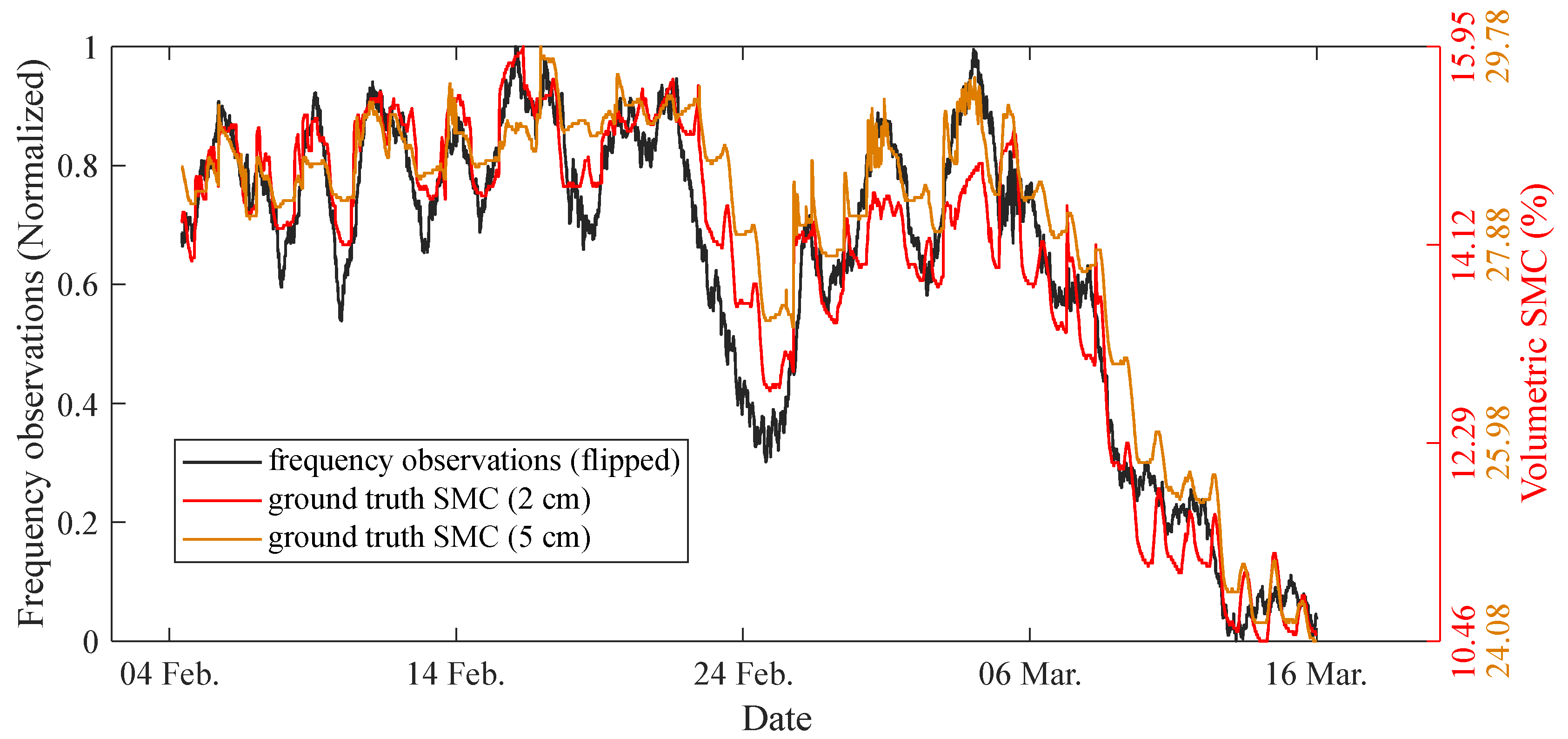
Figure 12 shows the correlation between ground truth measurements and frequency observations obtained from the proposed SNR model.
The frequency variation was inversely proportional to soil moisture variation, as reported in [12,21]. The correlation coefficient between frequency observations and 2-cm SMC was improved to 0.9548 (absolute value, ) as compared with previous work [21], which was 0.90 (, 2-cm SMC). Bad data points of only 4.27% were discarded before giving the results shown in Figure 12.
The correlation coefficient between ground truth SMC and phase observations obtained from the proposed SNR model was also calculated. The resulting correlation was 0.9301 with , which was slightly degraded compared with the value from previous work, which was 0.95 (, 2-cm SMC). The results could not be expected to be improved because the reduced phase estimation error achieved by the proposed SNR model was only 1.0113 × 10, which can be neglected according to the simulation results shown in Section 4.2. Finally, bad data points of only 5.20% were discarded before giving the correlation results.
The experimental results are summarized in Table 2.
6. Discussion
6.1. Choice of Fitting Function
In the proposed model, we use a polynomial function to describe the decibel variation of the signal power, which naturally results in a combination of the polynomial function and exponential function in Equation (8). In general, it is free to choose the form of the exponential function. Through testing, the following exponential functions gave the same QoF:
The basic design principle is that the signal power should always be positive. The exponential function is one of the functions that possesses this property. The first function in Equation (15) was finally chosen because both the function itself and its base-10 logarithm have physical significance.
6.2. Retrieval Ambiguity
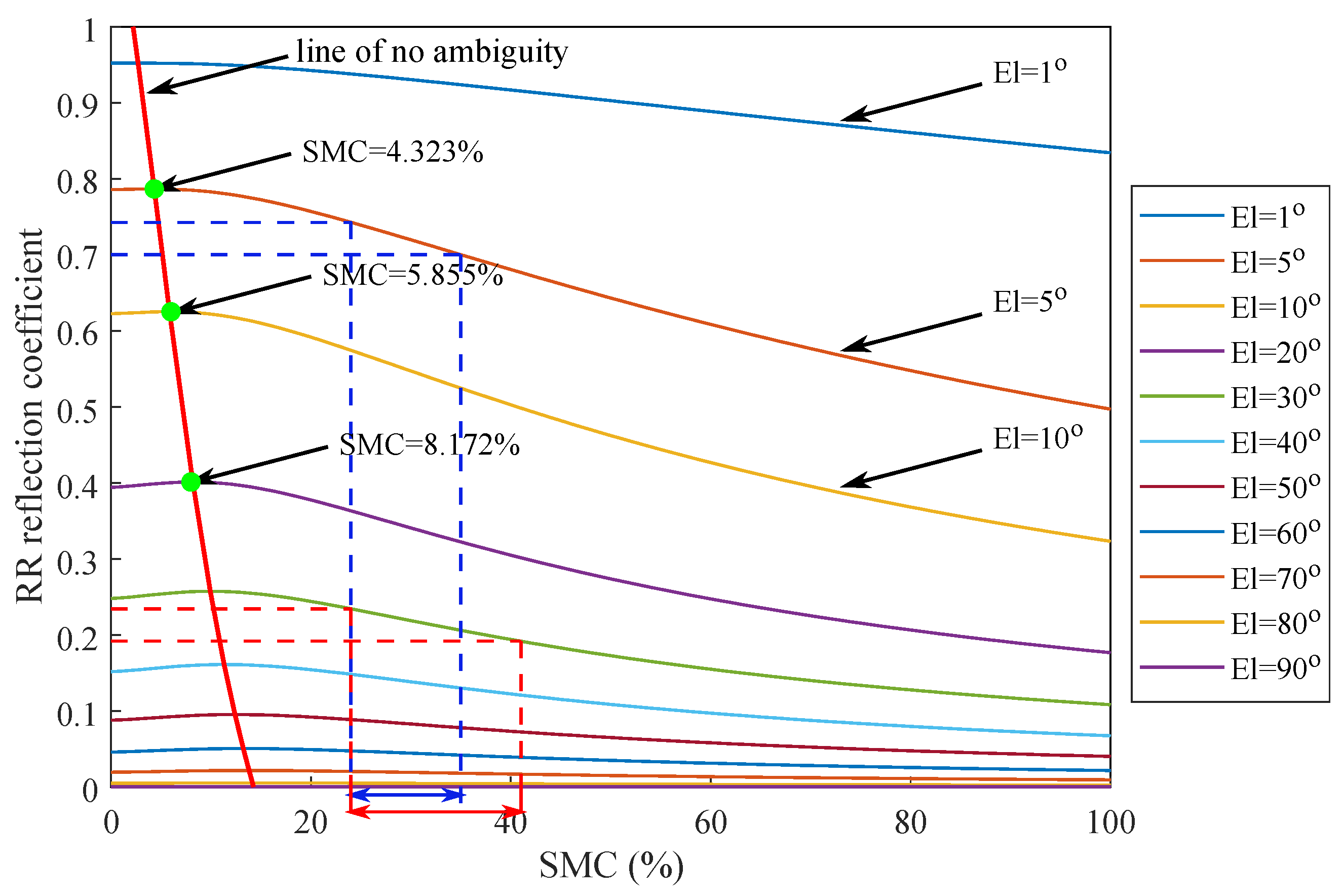
An ambiguity problem was encountered in retrieval using the reconstructed reflection coefficient. It is illustrated in Figure 13.
Figure 13 shows that the relationship between the RR reflection coefficient and soil moisture was not monotonic. When there was little soil moisture, the reflection coefficient increased slightly with soil moisture. However, after a certain point, which was determined by the elevation angle, this relationship became inverse. This means that one reflection coefficient might be associated with two soil moisture values, which would give rise to the ambiguity problem. To clarify this, a red line was plotted to indicate the points that have no ambiguity problem. In Section 5.1, the retrieval was performed at a 10° elevation angle, so the point with no ambiguity was located at 5.855% soil moisture. Furthermore, data from ground truth measurements showed that the soil moisture was larger than 6% during the experiment period, so retrieval results that were below 6% were regarded as bad data points and were discarded in the processing. Though not shown in Figure 13, we have to mention that the ambiguity is essentially caused by the non-monotonic relation between the RR reflection coefficient and dielectric constant at fixed elevation angles.
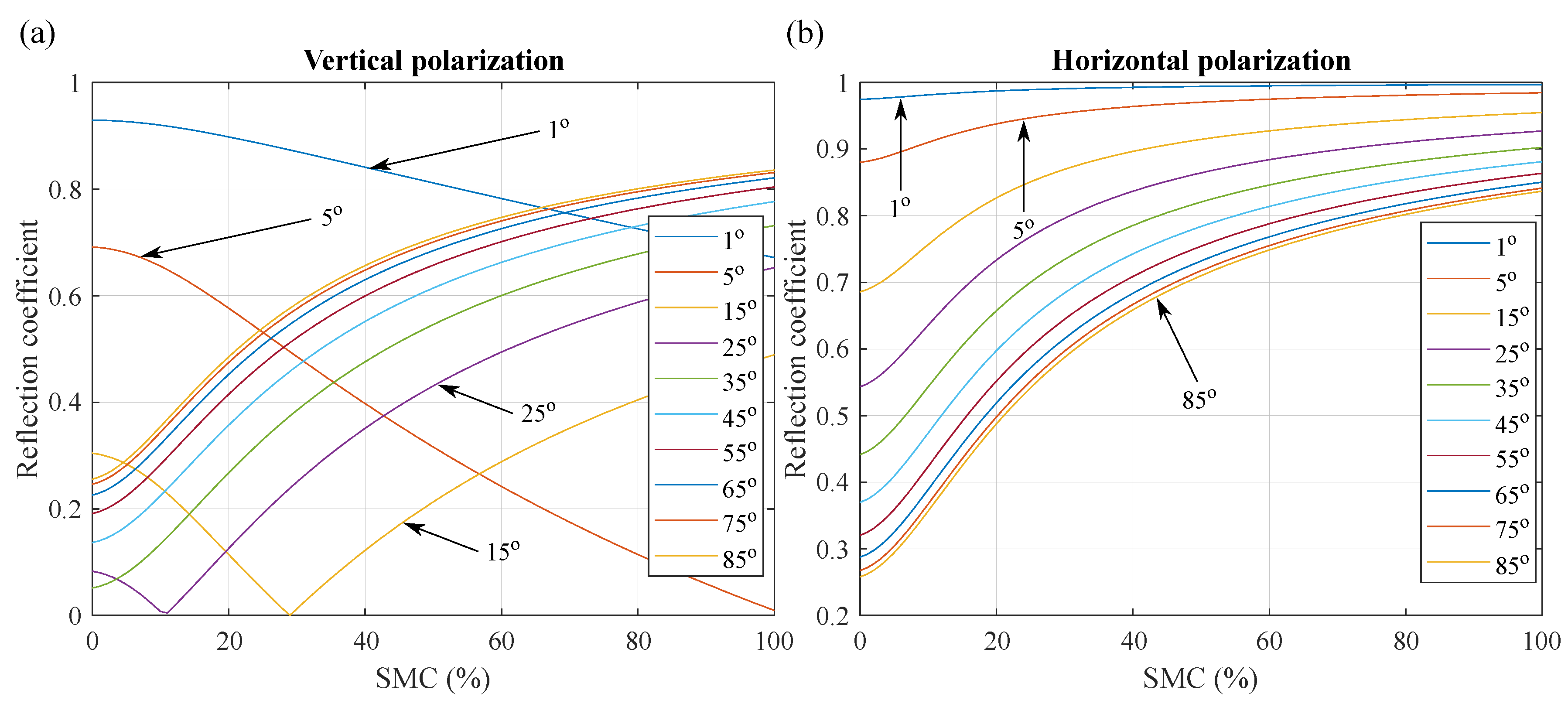
Since GNSS-IR using the linear polarized antenna configuration was also seen in the literature, two other linear polarized reflection coefficients were also studied. The results are shown in Figure 14.
As seen in Figure 14, vertical polarization shows no ambiguity problem when the elevation angle is above Brewster’s angle, which is near 30°, while horizontal polarization does not have this problem under any of the elevation angles.
6.3. Performance Analysis
In simulation and experimental data validation using a reconstructed reflection coefficient, two phenomena were observed: (1) the retrieval results statistically deviated from the true value; (2) it tended to give more bad results compared with the other two metrics (frequency and phase, as seen in Table 2). This indicated that the retrieval is not so robust, as reported in [28]. Possible explanations are as follows.
Several reasons cause the phenomenon in (1). Firstly, the noise on the SNR data is not Gaussian noise, seen from Equation (3). The Probability Density Function (PDF) of noise is changed after nonlinear operations such as square and division. This also results in the non-zero mean of noise. Under these situations, estimation results will deviate from the true value even if the model error is zero. Secondly, polynomial functions used in the SNR model cannot fully model the direct and reflected signal variation, especially when there is complex irregular variation caused by unpredictable factors. Thirdly, subsequent corrections such as antenna gain correction may not be accurate. The antenna gain used here was only obtained from two-dimensional measurements. We further assumed that the antenna gain was omnidirectional in the azimuth direction, but in reality, this was not the case. When the satellite is moving around, the transmitted signal will enter the antenna from a different azimuth direction, and the imperfect azimuthal antenna gain pattern probably cannot be ignored. For example, the ascending and descending paths of a satellite usually have a big difference regarding their azimuth angle range. Under this situation, the imperfect azimuthal antenna gain will result in a big difference between the retrieved SMC from the two paths, for instance the SMC estimation errors from the ascending and descending path of PRN No. 7 have a big difference as shown in Figure 9. Moreover, every antenna has cross-polarization [29]. For this reason, the LHCP component of the reflected signal could also enter the antenna and interfere with the direct signal, and we did not take this effect into consideration either. Finally, Hallikainen’s dielectric model used here may not be accurate. This dielectric model was developed based on the data collected from the five types of soil at room temperature (23 °C) [17]. The soil type in this experiment is silt clay, which fit in one of the five soil types; however, the soil temperature in the period of this experiment varied between 5 °C and 16 °C. Therefore, this would introduce some error. Recent studies suggested using the more complicated Mironov model, which incorporated the temperature parameter into the model and was tested on a wider range of soil types [30,31]. Although all these factors contribute to the error, the effect of the SNR model error and inaccurate corrections are most significant.
Error sensitivity caused the phenomenon in (2). As shown in Figure 13, the blue and red dashed lines illustrate the problem. For SMC retrieval using the RR reflection coefficient, a small error in reflection coefficient estimation can cause large errors in SMC estimation, which means that the result is very sensitive to error or noise. This effect is even worse for very low and very high elevation angles, which can explain why the standard deviation of errors was even worse at both ends in Figure 5b. The elevation angle we chose in this processing was 10°; its error sensitivity is relatively weak.
7. Conclusions
In this paper, the GNSS-IR (Global Navigation Satellite System-Interferometry and Reflectometry) soil moisture retrieval technique was studied. A semi-empirical SNR model was designed to fit with SNR data routinely collected by a GNSS receiver in a least square sense. One of the advantages of this model is that the direct and reflected signal can be reconstructed from SNR data with little prior knowledge needed. At the same time, the quality of fit can be improved causing the better estimation of frequency and phase information, which were widely recognized as good indicators of soil moisture variation. The main idea of this design is to approximate the direct and reflected signal by a second-order and fourth-order polynomial, respectively, based on the well-established SNR model. Both simulation and experimental data analysis were carried out to validate the model performance, and the results were compared with that obtained using the Larson model. Particularly, the simulation was performed considering the noise effect. The main results and findings were as follows:
Firstly, simulation results statistically showed that soil permittivity could be estimated from the reconstructed signals. The soil moisture retrieval was satisfactory in a specific elevation angle range such as from 5° to 15°. However, this process suffer from the ambiguity problem when the true soil moisture was very low (∼0.06 ). In addition, the estimation accuracy of frequency and phase was also slightly improved since the proposed SNR model improved the quality of fit from 55% to 95%. However, it was found that the improvement on phase estimation could be neglected.
Secondly, experimental data validation showed that it tended to give more bad results in soil moisture retrieval using reconstructed signals under the effect of model error and non-zero mean and non-Gaussian noise. This roots from the the error sensitivity of the reflection coefficient regarding the right-handed circular polarization. The most accurate estimation was given by PRN No. 15 during its descending period, with RMSE of 0.0446 . Furthermore, the correlation coefficient between the retrieved soil moisture and ground truth measurements was increased by at least 0.15, as compared with the correlation calculated from the SNR amplitude based on the same dataset. This improvement mainly benefited from appropriate modeling of the signal interference that was ignored in the Larson model. Two other obtained SNR metrics (frequency and phase) were also tested using the same dataset to study the performance of the proposed model. Results showed that the correlation coefficient between estimated frequency and ground truth measurements was improved from 90% to 95%, while the correlation coefficient calculated from phase measurement was slightly degraded from 95% to 93%. Some of the results were qualitatively in accordance with the simulation.
Further effort should be focused on improving the QoF even under more complicated irregular SNR variation through fitting function design. We next aim at identifying the source of these irregular variations and incorporating them into the subsequent retrieval model. In addition, the retrieval model used currently still needs further refinement to improve the accuracy of reflection coefficient estimation, including more accurate antenna gain correction and cross-polarization suppression, etc. Furthermore, the simulation carried out in this paper only considered white noise, and further simulation study should take speckle noise into consideration if the surface height variation is comparable to one wavelength or if ribbings/ridges are formed during the farming period. Since this proposed SNR model could capture high-order nonlinear SNR variation, it might be used to monitor vegetation in the future.
Acknowledgments
The authors would like to thank F. Baup and K. Boniface for collecting the meteorological data, as well as Roussel and F. Frappart for collecting GNSS observation data. The authors are also grateful to J. Darrozes for providing the data. This work was supported by the National Natural Science Foundation of China (No. 41774028), the National Key Research and Development (R&D) Plan (No. 2017YFB0502802), the Cross Disciplinary Cooperation Project of Beijing Science and Technology New Star Program (No. xxjc201603), the Open Project of National Engineering Research Center for Information Technology in Agriculture (No. KF2015W003) and the Beidou Technology Transformation and Industrialization grant of Beihang University (No. BARI1709).
Author Contributions
M. Han proposed the approach and drafted the manuscript. Y. Zhu organized the architecture of the paper. D. Yang carried out the simulations. X. Hong processed the data. S. Song analyzed the results. all of the authors contributed to the discussion.
Conflicts of Interest
The authors declare no conflict of interest.
Abbreviations
The following abbreviations are used in this manuscript:
| GNSS | Global Navigation Satellite System |
| GNSS-R | GNSS Reflectometry |
| GNSS-IR | GNSS Interferometry and Reflectometry |
| GPS | Global Positioning System |
| SNR | Signal-to-Noise Ratio |
| IPT | Interference Pattern Technique |
| SMC | Soil Moisture Content |
| QoF | Quality of Fit |
| RMSE | Root-Mean-Square Error |
| ME | Mean Error |
| Probability Density Function | |
| RHCP | Right-Handed Circularly Polarized |
| LHCP | Left-Handed Circularly Polarized |
| V-POL | Vertical-Polarized |
| H-POL | Horizontal-Polarized |
| MLE | Maximum Likelihood Estimate |
| AGC | Automatic Gain Control |
| PRN | Pseudo-Random Noise |
| RF | Radio Frequency |
| LSQ | Least SQuare |
| RR | RHCP to RHCP |
References
- Derksen, C.; Xu, X.; Dunbar, R.S.; Colliander, A.; Kim, Y.; Kimball, J.S.; Black, T.A.; Euskirchen, E.; Langlois, A.; Loranty, M.M.; et al. Retrieving Landscape Freeze/Thaw State from Soil Moisture Active Passive (SMAP) Radar and Radiometer Measurements. Remote Sens. Environ. 2017, 194, 48–62. [Google Scholar] [CrossRef]
- Alonso-Arroyo, A.; Torrecilla, S.; Querol, J.; Camps, A.; Pascual, D.; Park, H.; Onrubia, R. Two Dedicated Soil Moisture Experiments Using the Scatterometric Properties of GNSS-Reflectometry. In Proceedings of the 2015 IEEE International Geoscience and Remote Sensing Symposium (IGARSS), Milan, Italy, 26–31 July 2015; pp. 3921–3924. [Google Scholar]
- Katzberg, S.J.; Torres, O.; Grant, M.S.; Masters, D. Utilizing Calibrated GPS Reflected Signals to Estimate Soil Reflectivity and Dielectric Constant: Results from SMEX02. Remote Sens. Environ. 2006, 100, 17–28. [Google Scholar] [CrossRef]
- Sánchez, N.; Alonso-Arroyo, A.; Martínez-Fernández, J.; Piles, M.; González-Zamora, Á.; Camps, A.; Vall-llosera, M. On the Synergy of Airborne GNSS-R and Landsat 8 for Soil Moisture Estimation. Remote Sens. 2015, 7, 9954–9974. [Google Scholar] [CrossRef] [Green Version]
- Carreno-Luengo, H.; Lowe, S.; Zuffada, C.; Esterhuizen, S.; Oveisgharan, S. Spaceborne GNSS-R from the SMAP Mission: First Assessment of Polarimetric Scatterometry over Land and Cryosphere. Remote Sens. 2017, 9, 2072–4292. [Google Scholar] [CrossRef]
- Egido, A.; Caparrini, M.; Ruffini, G.; Paloscia, S.; Santi, E.; Guerriero, L.; Pierdicca, N.; Floury, N. Global Navigation Satellite Systems Reflectometry as a Remote Sensing Tool for Agriculture. Remote Sens. 2012, 4, 2356–2372. [Google Scholar] [CrossRef]
- Ulaby, F.T.; Long, D.G.; Blackwell, W.; Sarabandi, K.; Elachi, C. Microwave Radar and Radiometric Remote Sensing; Artech House: Norwood, MA, USA, 2013. [Google Scholar]
- Larson, K.M.; Small, E.E.; Gutmann, E.; Bilich, A.; Axelrad, P.; Braun, J. Using GPS Multipath to Measure Soil Moisture Fluctuations: Initial Results. GPS Solut. 2008, 12, 173–177. [Google Scholar] [CrossRef]
- Rodriguez Alvarez, N.; Aguasca, A.; Valencia, E.; Bosch, X.; Ramos-Perez, I.; Park, H.; Camps, A.; Vall-llossera, M. Snow Monitoring Using GNSS-R Techniques. In Proceedings of the 2011 International Geoscience and Remote Sensing Symposium (IGARSS), Vancouver, BC, Canada, 24–29 July 2011; pp. 4375–4378. [Google Scholar]
- Roussel, N.; Ramillien, G.; Frappart, F.; Darrozes, J.; Gay, A.; Biancale, R.; Striebig, N.; Hanquiez, V.; Bertin, X.; Allain, D. Sea level Monitoring and Sea State Estimate Using a Single Geodetic Receiver. Remote Sens. Environ. 2015, 171, 261–277. [Google Scholar] [CrossRef]
- Larson, K.M.; Braun, J.J.; Small, E.E.; Zavorotny, V.U.; Gutmann, E.D.; Bilich, A.L. GPS Multipath and Its Relation to Near-Surface Soil Moisture Content. IEEE J. Sel. Top. Appl. Earth Obs. Remote Sens. 2010, 3, 91–99. [Google Scholar] [CrossRef]
- Chew, C.; Small, E.E.; Larson, K.M.; Zavorotny, V.U. Effects of Near-Surface Soil Moisture on GPS SNR Data: Development of a Retrieval Algorithm for Soil Moisture. IEEE Trans. Geosci. Remote Sens. 2014, 52, 537–543. [Google Scholar] [CrossRef]
- Chew, C.; Small, E.E.; Larson, K.M. An Algorithm for Soil Moisture Estimation Using GPS-Interferometric Reflectometry for Bare and Vegetated Soil. GPS Solut. 2016, 20, 525–537. [Google Scholar] [CrossRef]
- Rodriguez-Alvarez, N.; Bosch-Lluis, X.; Camps, A.; Vall-Llossera, M.; Valencia, E.; Marchan-Hernandez, J.F.; Ramos-Perez, I. Soil Moisture Retrieval Using GNSS-R Techniques: Experimental Results Over a Bare Soil Field. IEEE Trans. Geosci. Remote Sens. 2009, 47, 3616–3624. [Google Scholar] [CrossRef]
- Arroyo, A.A.; Camps, A.; Monerris, A.; Rüdiger, C.; Walker, J.P.; Forte, G.; Pascual, D.; Park, H.; Onrubia, R. The Dual Polarization GNSS-R Interference Pattern Technique. In Proceedings of the 2014 International Geoscience and Remote Sensing Symposium (IGARSS), Quebec City, QC, Canada, 13–18 July 2014; pp. 3921–3924. [Google Scholar]
- Arroyo, A.A.; Camps, A.; Aguasca, A.; Forte, G.F.; Monerris, A.; Rüdiger, C.; Walker, J.P.; Park, H.; Pascual, D.; Onrubia, R. Dual-Polarization GNSS-R Interference Pattern Technique for Soil Moisture Mapping. IEEE J. Sel. Top. Appl. Earth Obs. Remote Sens. 2014, 7, 1533–1544. [Google Scholar] [CrossRef]
- Hallikainen, M.T.; Ulaby, F.T.; Dobson, M.C.; El-rayes, M.A.; Wu, L. Microwave Dielectric Behavior of Wet Soil-Part 1: Empirical Models and Experimental Observations. IEEE Trans. Geosci. Remote Sens. 1985, GE-23, 25–34. [Google Scholar] [CrossRef]
- Wang, J.R.; Schmugge, T.J. An Empirical Model for the Complex Dielectric Permittivity of Soils as a Function of Water Content. IEEE Trans. Geosci. Remote Sens. 1980, GE-18, 288–295. [Google Scholar] [CrossRef]
- Yang, T.; Wan, W.; Chen, X.; Chu, T.; Hong, Y. Using BDS SNR Observations to Measure Near-Surface Soil Moisture Fluctuations: Results From Low Vegetated Surface. IEEE Geosci. Remote Sens. Lett. 2017, 14, 1308–1312. [Google Scholar] [CrossRef]
- Zavorotny, V.U.; Larson, K.M.; Braun, J.J.; Small, E.E.; Gutmann, E.D.; Bilich, A.L. A Physical Model for GPS Multipath Caused by Land Reflections: Toward Bare Soil Moisture Retrievals. IEEE J. Sel. Top. Appl. Earth Obs. Remote Sens. 2010, 3, 100–110. [Google Scholar] [CrossRef]
- Roussel, N.; Frappart, F.; Ramillien, G.; Darrozes, J.; Baup, F.; Lestarquit, L.; Ha, M.C. Detection of Soil Moisture Variations Using GPS and GLONASS SNR Data for Elevation Angles Ranging From 2° to 70°. IEEE J. Sel. Top. Appl. Earth Obs. Remote Sens. 2016, 9, 4781–4794. [Google Scholar] [CrossRef]
- Kaplan, E.D.; Hegarty, C. Understanding GPS: Principles and Application; Artech House: Norwood, MA, USA, 2005. [Google Scholar]
- Satyanarayana, S.; Borio, D.; Lachapelle, G. C/N0 Estimation: Design Criteria and Reliability Analysis Under Global Navigation Satellite System (GNSS) Weak Signal Scenarios. IET Radar Sonar Navig. 2012, 6, 81–89. [Google Scholar] [CrossRef]
- Roussel, N.; Frappart, F.; Ramillien, G.; Darrozes, J.; Desjardins, C.; Gegout, P.; Pérosanz, F.; Biancale, R. Simulations of Direct and Reflected Wave Trajectories for Ground-Based GNSS-R Experiments. Geosci. Model Dev. 2014, 7, 2261–2279. [Google Scholar] [CrossRef] [Green Version]
- Masters, D.; Axelrad, P.; Katzberg, S. Initial Results of Land-Reflected GPS Bistatic Radar Measurements in SMEX02. Remote Sens. Environ. 2004, 92, 507–520. [Google Scholar] [CrossRef]
- Stutzman, W. Polarization in Electromagnetic Systems; Artech House: Norwood, MA, USA, 1993. [Google Scholar]
- Davies, H. The Reflection of Electromagnetic Waves From a Rough Surface. Proc. IEE Part III Radio Commun. Eng. 1954, 101, 209–214. [Google Scholar] [CrossRef]
- Peng, X.; Wan, W.; Chen, X. Using GPS SNR Data to Estimate Soil Moisture Variations: Proposing a New Interference Model. In Proceedings of the 2016 IEEE International Geoscience and Remote Sensing Symposium (IGARSS), Beijing, China, 10–15 July 2016; pp. 4819–4822. [Google Scholar]
- Kraus, J.D.; Marhefka, R.J. Antennas For All Applications; McGraw-Hill: Columbus, OH, USA, 2003. [Google Scholar]
- Mironov, V.L.; Fomin, S.V. Temperature and Mineralogy Dependable Model for Microwave Dielectric Spectra of Moist Soils. Piers Online 2009, 5, 411–415. [Google Scholar] [CrossRef]
- Wigneron, J.P.; Chanzy, A.; Kerr, Y.H.; Lawrence, H.; Shi, J.; Escorihuela, M.J.; Mironov, V.; Mialon, A.; Demontoux, F.; de Rosnay, P.; et al. Evaluating an Improved Parameterization of the Soil Emission in L-MEB. IEEE Trans. Geosci. Remote Sens. 2011, 49, 1177–1189. [Google Scholar] [CrossRef]
Figure 1.
Typical multipath reflection geometry.

Figure 2.
The overall retrieval procedure.

Figure 3.
Antenna gain pattern.

Figure 4.
Reconstruction results.

Figure 5.
Statistical results of SMC retrieval under different satellite elevation angles and coherent accumulation M. (a) Mean; (b) standard deviation.
Figure 5.
Statistical results of SMC retrieval under different satellite elevation angles and coherent accumulation M. (a) Mean; (b) standard deviation.

Figure 6.
A mean absolute estimation error comparison between the proposed model and the Larson model. (a) Frequency estimation error; (b) phase estimation error.
Figure 6.
A mean absolute estimation error comparison between the proposed model and the Larson model. (a) Frequency estimation error; (b) phase estimation error.

Figure 7.
Fitting results of GPS PRN No. 4. (a) Ascending path; (b) Descending path.

Figure 8.
Retrieval results obtained from the reconstructed signal. (a) Results obtained from the ascending path of PRN No. 7; and (b) results obtained from the descending path of PRN No. 15.
Figure 8.
Retrieval results obtained from the reconstructed signal. (a) Results obtained from the ascending path of PRN No. 7; and (b) results obtained from the descending path of PRN No. 15.

Figure 9.
Valid results obtained from the reconstructed signal for all the satellites.

Figure 10.
Normalized, combined and smoothed results.

Figure 11.
Fitting results of some parts of the simulated SNR.

Figure 12.
Normalized, combined and smoothed results using frequency observation.

Figure 13.
Retrieval ambiguity.

Figure 14.
Relationship between SMC and linear polarized reflection coefficient under different elevation angles. (a) Vertical polarization; and (b) horizontal polarization.
Figure 14.
Relationship between SMC and linear polarized reflection coefficient under different elevation angles. (a) Vertical polarization; and (b) horizontal polarization.


Table 1.
Other simulation settings.
| Parameter | Value | Unit |
|---|---|---|
| Carrier Frequency | 1575.42 | MHz |
| Carrier Signal Power | −160 | dBw |
| Single Sideband Power Spectrum Density | –205.2 | dBw/Hz |
| Front-end Bandwidth B | 2.046 | MHz |
| Antenna Height H | 2 | m |
| Satellite Elevation Angle Changing Rate | 1.16347 × 10 | rad/s |
| Satellite Elevation Angle Range | deg | |
| Volumetric Soil Moisture Content SMC | 0.2785 | |
| Proportion of Sand in Soil S | 18 | % |
| Proportion of Clay in Soil C | 41 | % |
| Polynomial Order , | 2, 4 | |
| Number of Coherent Accumulation M | 2, 10, 20, 100, 200, 300, ⋯, 1000 | ms |
| Number of Simulation Runs | 200 |
Table 2.
Correlation coefficient between SNR metrics and ground truth measurements.
| SNR Metrics | Reconstructed Reflection Coefficient | Frequency | Phase | ||
|---|---|---|---|---|---|
| Values | |||||
| Assessment | |||||
| Absolute correlation (2 cm/5 cm) | 0.8824/0.9370 () | 0.9548/0.9463 () | 0.9301/0.9036 () | ||
| Discarded bad data | 22.13% | 4.27% | 5.20% | ||
© 2018 by the authors. Licensee MDPI, Basel, Switzerland. This article is an open access article distributed under the terms and conditions of the Creative Commons Attribution (CC BY) license (http://creativecommons.org/licenses/by/4.0/).
Share and Cite
MDPI and ACS Style
Han, M.; Zhu, Y.; Yang, D.; Hong, X.; Song, S. A Semi-Empirical SNR Model for Soil Moisture Retrieval Using GNSS SNR Data. Remote Sens. 2018, 10, 280. https://doi.org/10.3390/rs10020280
AMA Style
Han M, Zhu Y, Yang D, Hong X, Song S. A Semi-Empirical SNR Model for Soil Moisture Retrieval Using GNSS SNR Data. Remote Sensing. 2018; 10(2):280. https://doi.org/10.3390/rs10020280
Chicago/Turabian StyleHan, Mutian, Yunlong Zhu, Dongkai Yang, Xuebao Hong, and Shuhui Song. 2018. "A Semi-Empirical SNR Model for Soil Moisture Retrieval Using GNSS SNR Data" Remote Sensing 10, no. 2: 280. https://doi.org/10.3390/rs10020280
Note that from the first issue of 2016, this journal uses article numbers instead of page numbers. See further details here.