An Automatic Random Forest-OBIA Algorithm for Early Weed Mapping between and within Crop Rows Using UAV Imagery

Abstract

Accurate and timely detection of weeds between and within crop rows in the early growth stage is considered one of the main challenges in site-specific weed management (SSWM). In this context, a robust and innovative automatic object-based image analysis (OBIA) algorithm was developed on Unmanned Aerial Vehicle (UAV) images to design early post-emergence prescription maps. This novel algorithm makes the major contribution. The OBIA algorithm combined Digital Surface Models (DSMs), orthomosaics and machine learning techniques (Random Forest, RF). OBIA-based plant heights were accurately estimated and used as a feature in the automatic sample selection by the RF classifier; this was the second research contribution. RF randomly selected a class balanced training set, obtained the optimum features values and classified the image, requiring no manual training, making this procedure time-efficient and more accurate, since it removes errors due to a subjective manual task. The ability to discriminate weeds was significantly affected by the imagery spatial resolution and weed density, making the use of higher spatial resolution images more suitable. Finally, prescription maps for in-season post-emergence SSWM were created based on the weed maps—the third research contribution—which could help farmers in decision-making to optimize crop management by rationalization of the herbicide application. The short time involved in the process (image capture and analysis) would allow timely weed control during critical periods, crucial for preventing yield loss.

1. Introduction

In recent years, images acquired by Unmanned Aerial Vehicles (UAVs) have proven their suitability for the early weed detection in crops [1,2,3]. This ability is even effective in challenging scenarios, such as weed detection in early season herbaceous crops, when the small plants of crop and weeds have high spectral similarity [4,5]. The success of UAV imagery for early season weed detection in herbaceous crops is based on three main factors: (1) images can be acquired at the most crucial agronomic moment for weed control (early post-emergence) due to the high flexibility of UAV flight scheduling; (2) orthomosaics generated from UAV images have very high spatial resolution (pixels < 5 cm) because UAVs can fly at low altitudes, making the detection of plants (crop and weeds) possible, even at the earliest phenological stage; and (3) UAV imagery acquisition with high overlaps permits the generation of Digital Surface Models (DSMs) by using photo-reconstruction techniques [6]. Such UAV-based DSMs have recently been used for different objectives in herbaceous crops. For example, Bendig et al. [7] created crop height models to estimate fresh and dry biomasses at a barley test site, Geipel et al. [8] combined crop surface models with spectral information to model corn yield, Iqbal et al. [9] employed DSM-based crop height to estimate the capsule volume of poppy crops, and Ostos et al. [10] calculated bioethanol potential via high-throughput phenotyping in cereals.

In addition, in early season agronomic scenarios, where crop and weed seedling show similar spectral signatures, the development of Object Based Image Analysis (OBIA) techniques allows better classification results to be obtained, compared to traditional pixel-based image analysis [11]. OBIA overcomes some of the limitations of pixel-based methods by segmenting the images into groups of adjacent pixels with homogenous spectral values and then using these groups, called “objects”, as the basic elements of its classification analysis [12]. OBIA techniques then combine spectral, topological, and contextual information from these objects to address challenging classification scenarios [11]. Therefore, the combination of UAV imagery and OBIA has enabled the significant challenge of automating early weed detection in early season herbaceous crops to be tackled [11,13], which represents a great advance in weed science. To achieve this goal, subsequent issues have been consecutively addressed: the discrimination of bare soil and vegetation; the detection of crop rows; and the detection of weeds, assuming that they are the vegetation objects growing outside the crop rows. However, the automatic detection of weeds growing inside the crop rows still remains an open challenge. In this context, Pérez-Ortiz et al. [3,14] used a Support Vector Machine (SVM) to map weeds within the crop rows, although user intervention for manual training patterns selection was required, which is time intensive and consequently, expensive, and could be a subjective task [15].

A variety of classification methods have been used to map weeds from UAV images. In recent years, especially for large dimensional and complex data, machine learning algorithms have emerged as more accurate and efficient alternatives to conventional parametric algorithms [16]. Among the multiple machine learning algorithms, the Random Forest classifier (RF) has received increasing attention from the remote sensing community due to its generalized performance and fast operation speed [16,17,18]. RF is an ensemble of classification trees, where each decision tree employs a subset of training samples and variables selected by a bagging approach, while the remaining samples are used for internal cross-validation of the RF performance [19]. The classifier chooses the membership classes having the most votes, for a given case [20]. Whereas RF only requires two parameters to be defined to generate the model [21], other machine learning techniques (e.g., neural networks and support vector machines) are difficult to automate. Reasons for this are the larger number of critical parameters that need to be set [22,23], and a tendency to over-fit the data [24]. Moreover, RF has been shown to be highly suitable for high resolution UAV data classification [25,26], suggesting that, in most cases, it should be considered for agricultural mapping [21].

As per the above discussion, the main objective of this work was the early season weed detection between and within rows in herbaceous crops, for the purpose of designing an in-season early post-emergence prescription map. To achieve this objective, we developed a new OBIA algorithm to create an RF classifier without any user intervention. Another original contribution is the use of plant height, which is calculated from the UAV-based DSMs, as an additional feature for weeds and crop discrimination.

2. Materials and Methods

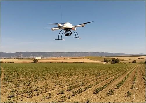
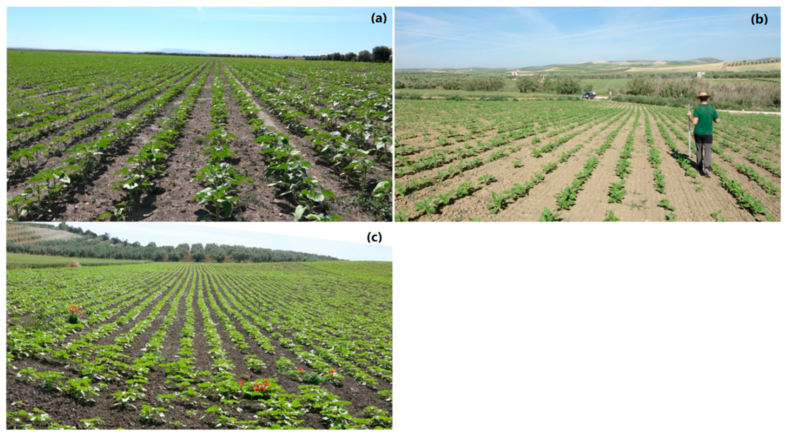
2.1. Study Site and UAV Flights

The experiments were carried out in three sunflower fields and two cotton fields, located in Córdoba and Sevilla provinces (Southern Spain). An overview of the study site characteristics and UAV flights can be found in

Table 1. Study fields and UAV-flight data.

Crop	Name	Flight Date	Crop Row Separation (m)	Area (ha)	Weed Validation Frames
Sunflower	S1–16	June 2016	0.8	4.22	107
	S1–17	May 2017	0.7	1.03	26
	S2–17	May 2017	0.7	1.56	37
Cotton	C1–16	June 2016	0.95	1.13	31
	C2–16	June 2016	0.95	1.05	27

.

In the overflown sunflower fields (Figure 1), with flat ground (average slope < 1%), the crops were in the 17, 18 growth stage of the BBCH (Biologische Bundesantalt, Bundessortenamt and Chemische Industrie) scale [27]. However, a small area in the S1–16 field had plants at a slightly earlier development stages (15, 16 stage), resulting in a wider range of plant heights. All fields were naturally infested by bindweed (Convolvulus arvensis L.), turnsole (Chrozophora tinctoria (L.) A. Juss.), knotweed (Polygonum aviculare L.) pigweed (Amaranthus blitoides S. Wats.) and canary grass (Phalaris spp.), the most common being bindweed. In addition to these species, the S2–17 field also exhibited a low infestation of poppy (Papaver rhoeas L.).

Crop plants growing in the cotton fields (Figure 2), which were also flat, were in stage 17, 18 of the BBCH scale. These fields, naturally infested with bindweed, turnsole, pigweed, and cocklebur (Xanthium strumarium L.), were managed for furrow irrigation, showing a structure of furrows and ridges.

Crop row separation was similar for both cotton fields (Table 1), and it varied from 0.7 to 0.8 m in sunflower fields. Weed plants had a similar size or, in some cases, were even smaller than the crop plants, specially inside the crop row, in all the studied fields, which is a common scenario in the early crop growth stages [3,14].

The remote images were acquired through UAV flights at 30 and 60 m ground height using a quadcopter model MD4-1000 (microdrones GmhH, Siegen, Germany). Flight data are shown in Table 1. The UAV can fly either by remote control (1000 m control range) or autonomously, with the aid of its Global Navigation Satellite System (GNSS) receiver and its waypoint navigation system. The UAV is battery powered and can load any sensor weighing up to 1.25 kg. The images were acquired with a lightweight (413 g), modified, commercial, off-the-shelf camera, model Sony ILCE-6000 (Sony Corporation, Tokyo, Japan). The camera was modified to capture information in both NIR and visible light (green and red) through adding a 49-mm filter ring to the front nose of the lens, manufactured by the company Mosaicmill (Mosaicmill Oy, Vantaa, Finlandia), where a focus calibration process was carried out (http://www.mosaicmill.com/images/broad_band_camera.jpg). This model is composed of a 23.5 × 15.6 mm APS-C CMOS sensor, capable of acquiring 24 megapixel (6000 × 4000 pixels) spatial resolution images with 8-bit radiometric resolution (for each channel), and is equipped with a 20-mm fixed lens.

The flight routes were designed to take photos with a forward overlap of 93% and a side overlap of 60%, large enough to achieve the 3D reconstruction of crops, according to previous research [28]. The flight operations fulfilled the list of requirements established by the Spanish National Agency of Aerial Security, including the pilot license, safety regulations and limited flight distance [29].

This approach, consisting of two crops growing in five different sites, and using several flight dates, made it possible to analyze the frequent variability in these field conditions.

2.2. DSM and Orthomosaic Generation

Geomatic products, such as DSM and orthomosaics, were generated using Agisoft PhotoScan Professional Edition software (Agisoft LLC, St. Petersburg, Russia) version 1.2.4 build 1874. With the exception of the manual localization of six ground control points (GCP) in the corners and center of each field to georeference the DSM and the orthomosaic; the mosaic development process was fully automatic. To work in Real Time Kinematic (RTK) mode with centimetric positioning accuracy, each GCP was measured using two GNSS receivers. One of the receivers was a reference station from the GNSS RAP network from the Institute for Statistics and Cartography of Andalusia, Spain, and the other one was a rover receiver Trimble R4 (Trimble, Sunnyvale, CA, USA).

The DSM and orthomosaic generation involved three main steps: (1) aligning images; (2) building field geometry; and (3) ortho-photo generation. First, the software searched for common points in the images and matched them, to estimate the camera position in each image, and next the camera calibration parameters were calculated. Next, the dense 3D point cloud file was created by applying the Structure from Motion (SfM) technique to the images. On the basis of the estimated camera position and the images themselves, the DSM with height information was developed from the 3D point cloud (Figure 3). The DSM is a 3D polygon mesh that represents the overflown area, and reflects the irregular geometry of the ground as well as the plant shape. Finally, the individual images were projected over the DSM, and the orthomosaic was generated. The DSMs were saved in grayscale tiff format and joined to the orthomosaic, which produced a 4-band multi-layer file (Red, Green, NIR and DSM). More details about the Photoscan functioning are given in [30].

The orthomosaic pixel size was directly proportional to the flight altitude, with values of 0.6 cm at 30 m, and 1.2 cm at 60 m. Similarly, the DSM spatial resolution varied from 1.2 cm to 2.4 cm, for the 30 m and 60 m flight altitudes, respectively.

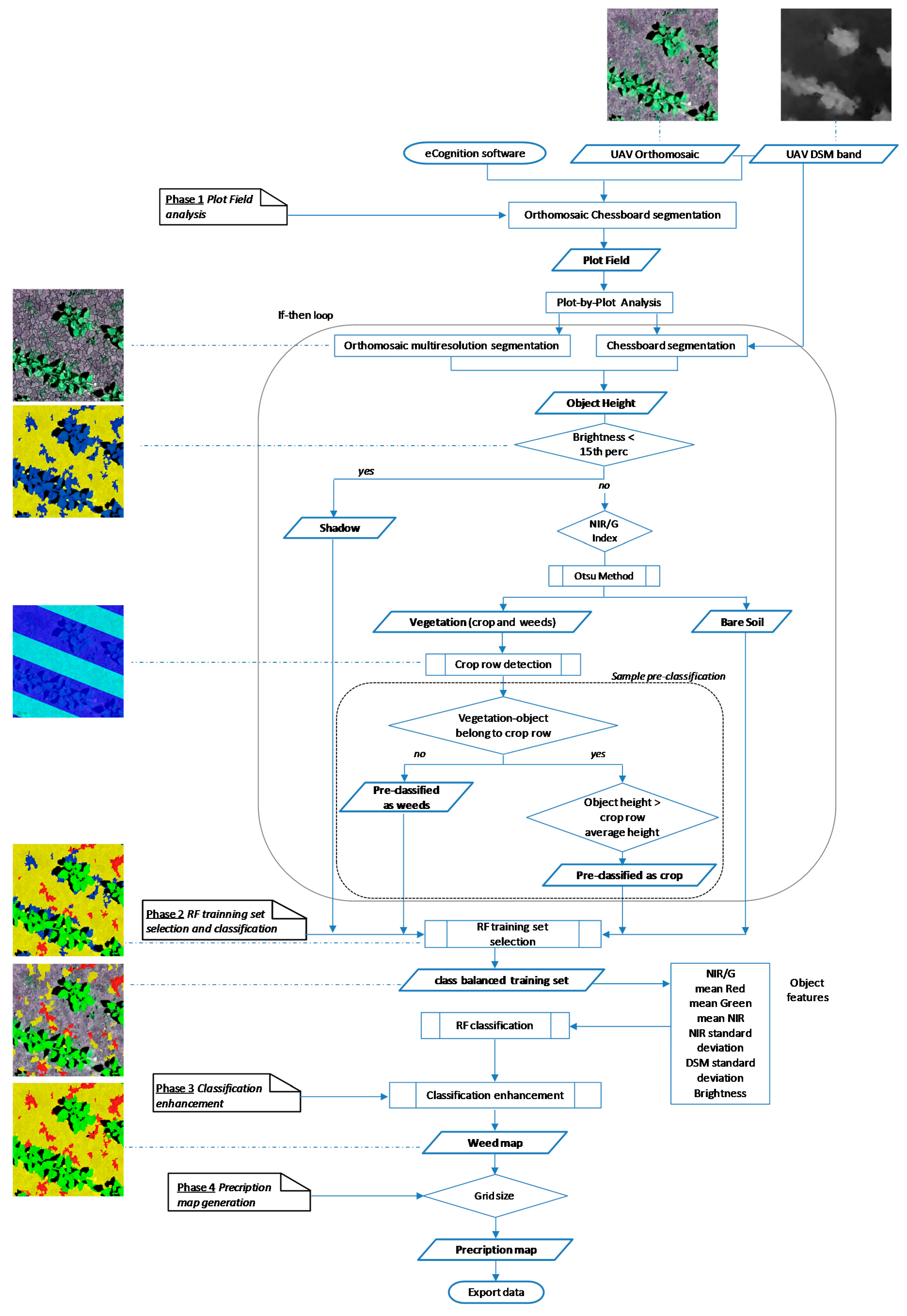
2.3. Image Analysis Algorithm Description

The OBIA algorithm for the detection of weeds was developed using the Cognition Network programming language with eCognition Developer 9 software (Trimble GeoSpatial, Munich, Germany). The algorithm was based on the versions fully described in our previous work, conducted in sunflower and maize fields [5,11,13]. These previous versions classified the vegetation growing outside the crop rows as weeds, and, consequently, the weeds within the crop row were not detected. Therefore, the new version presented here is original, and includes improvements to distinguish weeds both outside and within crop rows. Another novelty of the algorithm version presented here is that it automatically trains the samples that feed the RF process, without any user intervention.

The algorithm was composed of a sequence of phases (Figure 4), using the orthomosaic and DSM as inputs, which are described as follows.

2.3.1. Plot Field Analysis

The orthomosaic is segmented into small parcels by applying a chessboard segmentation process. The sub-parcel size is user-configurable, and, in this experiment, a 10 × 10 m² parcel size was selected. Each individual sub-parcel was automatically and sequentially analyzed to address the spatial and spectral variability of the crop:

• Object height calculation: A chessboard segmentation algorithm was used to segment the DSM of every sub-parcel into squares of 0.5 m. Then, the minimum height above sea level was calculated, to build the digital terrain model (DTM), i.e., a graphical representation of the terrain height. Next, the orthomosaic, containing the spectral and height information, was segmented, using the multiresolution segmentation algorithm (known as MRS) [31] (Figure 4). MRS is a bottom-up segmentation algorithm based on a pairwise region merging technique in which, on the basis of several parameters defined by the operator (scale, color/shape, smoothness/compactness), the image is subdivided into homogeneous objects.
  The scale parameter was fixed at 17, as obtained in a previous study, in which a large set of herbaceous crop plot imagery was tested by using a tool developed for scale value optimization, in accordance with [32]. This tool was implemented as a generic tool for the eCognition software in order to parameterize multi-scale image segmentation, enabling objectivity and automation of GEOBIA analysis. In addition, shape and compactness parameters were fixed to 0.4 and 0.5, respectively, to be well suited for vegetation detection by using UAV imagery [33].
  Once the objects were created, the height above the terrain was extracted from the Crop Height Model (CHM), which was calculated by subtracting the DTM from the DSM.
• Shadow removing: shadows were removed by using an overall intensity measurement given by the brightness feature, as shadows are less bright than vegetation and bare soil [34]. The 15th percentile brightness was used as the threshold to accurately select and remove shadow objects, based on previous studies (Figure 4).
• Vegetation thresholding: Once homogenous objects were created by MRS, vegetation (crop and weeds) objects were separated from bare soil by using the NIR/G band ratio. This is an easy to implement ratio, designed to detect structural and color differences in land classes [35], and is insensitive to soil effects, e.g., differences observed in this ratio have been used to separate vegetation and bare soil, as NIR reflectance is higher for vegetation than for bare soil, while more similar spectral values are shown for vegetation and bare soil when considering a broad waveband in the green region, which enhances these diferences [36]. The optimum ratio value for vegetation distinction was conducted using an automatic and iterative threshold approach, following the Otsu method [37], implemented in eCognition, in accordance with Torres-Sánchez et al. [28].
• Crop row detection: A new level was created to define the main orientation of the crop rows, where a merging operation was performed to create lengthwise vegetation objects following the shape of a crop row. In this operation, two candidate vegetation objects were merged only if the length/width ratio of the target object increased after the merging. Next, the largest-in-size object, with orientation close to row one, was classified as a seed object belonging to a crop row. Finally, the seed object grew in both directions, following the row orientation, and a looping merging process was performed until all the crop rows hit the parcel limits. This procedure is fully described in Peña et al. [38]. After a stripe was classified as a sunflower (or cotton) crop-line, the separation distance between rows was used to mask the adjacent stripes, to avoid misclassifying weed infestation as crop rows (Figure 4).
• Sample pre-classification: Once vegetation objects were identified, the algorithm searched for potential samples of crops and weeds in every sub-parcel. Inside the row, vegetation objects with an above average height, previously determined for each crop row as the average height of plants in a row, were pre-classified as crops. All vegetation objects outside the crop rows were classified as weeds (Figure 4). Weeds growing inside the row, regardless of height, could be properly classified in the next step.

The average height of the crop row was shown to be a suitable feature for sample selection, as most weeds growing within the crop row in this scenario are generally smaller than the crop plants.

2.3.2. RF Training Set Selection and Classification

Since the RF classifier should use a class balanced training set to be efficient [17], a random sampling process was implemented to pick the same number of objects per class in the whole image. Then, NIR/G, mean Red, mean Green, mean NIR, brightness, NIR standard deviation, and CHM standard deviation values were extracted for every object making up the training set, and used as features to discriminate weed, crop and bare soil, using the RF implemented in eCognition. These features were previously selected from a set of spectral, textural, contextual and morphological features and vegetation indices, using the Rattle (the R Analytical Tool to Learn Easily) package [39], which is a recognized tool that provides a toolbox for quickly trying out and comparing different machine learning methods on new data sets. A quantity of 500 decision trees were used in the training process, as this value has been proven to be an acceptable value when using RF classifier on remotely sensed data, according to Belgiu and Drăguţ [17]. To avoid any misclassification of large weeds between or within the rows, the object height was not included as a classification feature. Once the RF was trained, this classification algorithm was applied to the unclassified whole field (Figure 4).

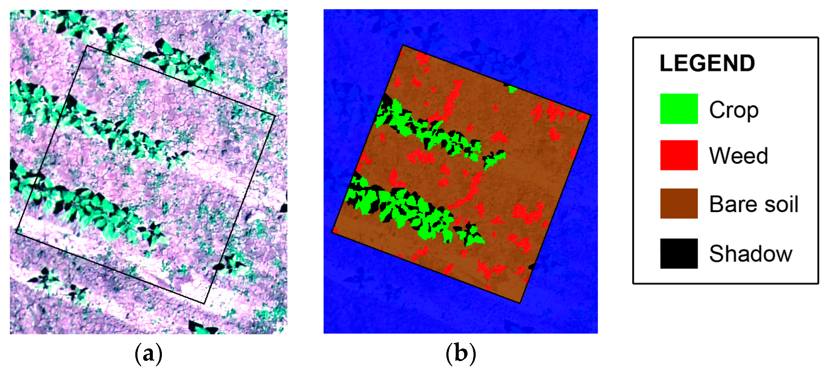
2.3.3. Classification Enhancement

As part of the automatic algorithm, a classification improvement was carried out by removing objects with anomalous spectral values, as follows: First, where the RF classifier had assigned objects to the wrong class in step 6, objects originally classified as bare soil in step 3 were correctly reclassified as bare soil; then, every object classified as crop outside the crop row was classified as a weed. Finally, the isolated small weed objects within the crop rows, and surrounded by bare soil or crops, were properly reclassified as crops (Figure 4).

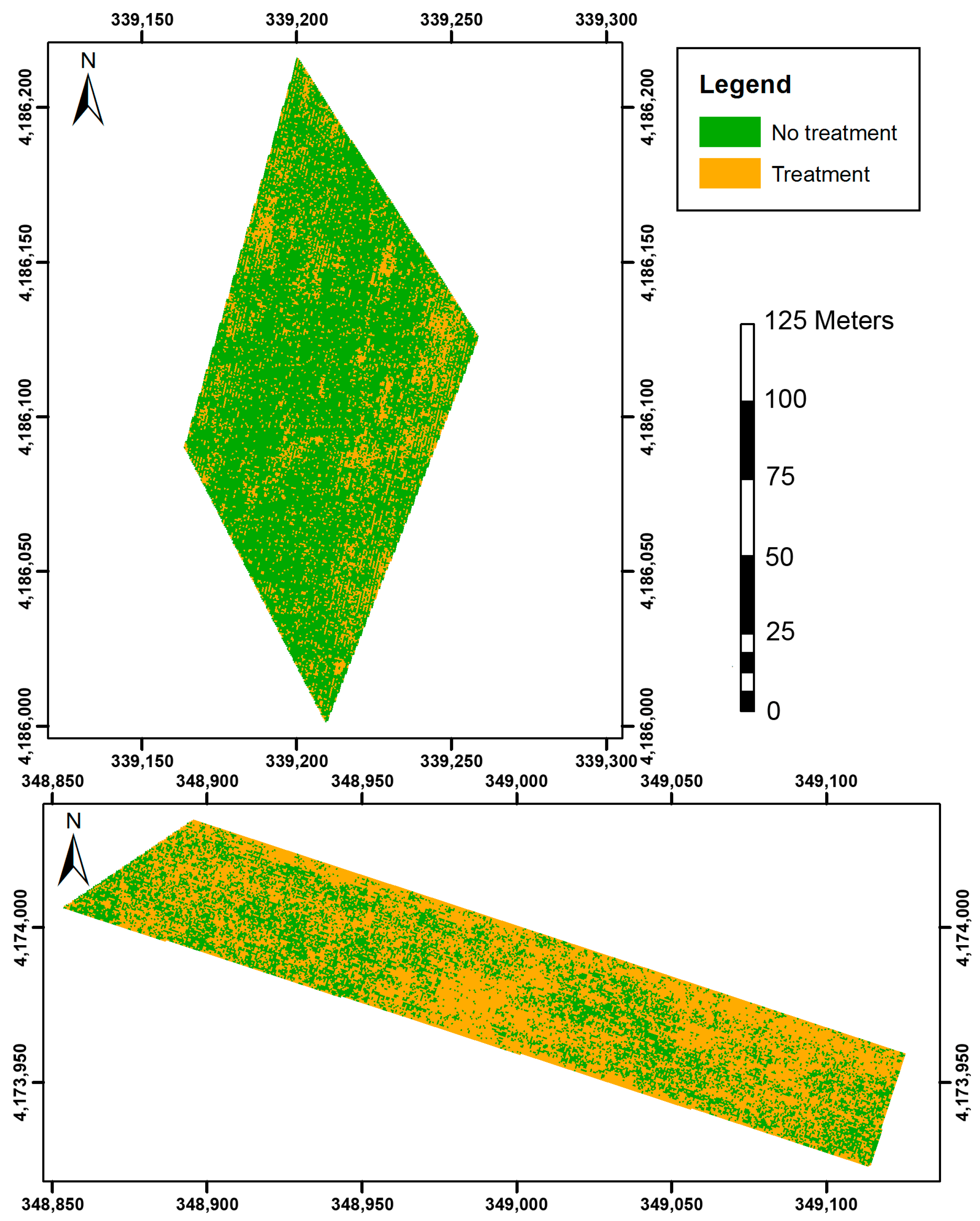
2.3.4. Prescription Map Generation

After weed–crop classification, the algorithm created a new level by copying the classified object level to an upper position in order to build a grid framework through the use of a chessboard segmentation process. The generated grid size is user-adjustable and follows the crop row orientation. In this experiment, a 0.5 × 0.5 m grid size was selected, in accordance with a site-specific sprayer prototype [40]. A new hierarchical structure was generated between the grid super-objects (upper level) and the crop-weed-bare soil classification (sub-objects at the lower level). Next, the grid with the presence of weeds in the lower level was marked as requiring control treatment.

2.4. Crop Height Validation

For every crop field and year, to measure the crop height of a set of validation points through the parcels, a systematic on-ground sampling procedure was conducted, resulting in 47 and 38 validation data points for sunflowers in 2016 and 2017, respectively, and 42 for cotton in 2016. Every validation point was georeferenced and photographed with the plant in front and the ruler included (Figure 5). The measured plant heights were compared to that calculated by the OBIA algorithm. The coefficient of determination (R²) derived from a linear regression model and the root mean square error (RMSE) of this comparison were calculated using JMP software (SAS, Cary, NC, USA).

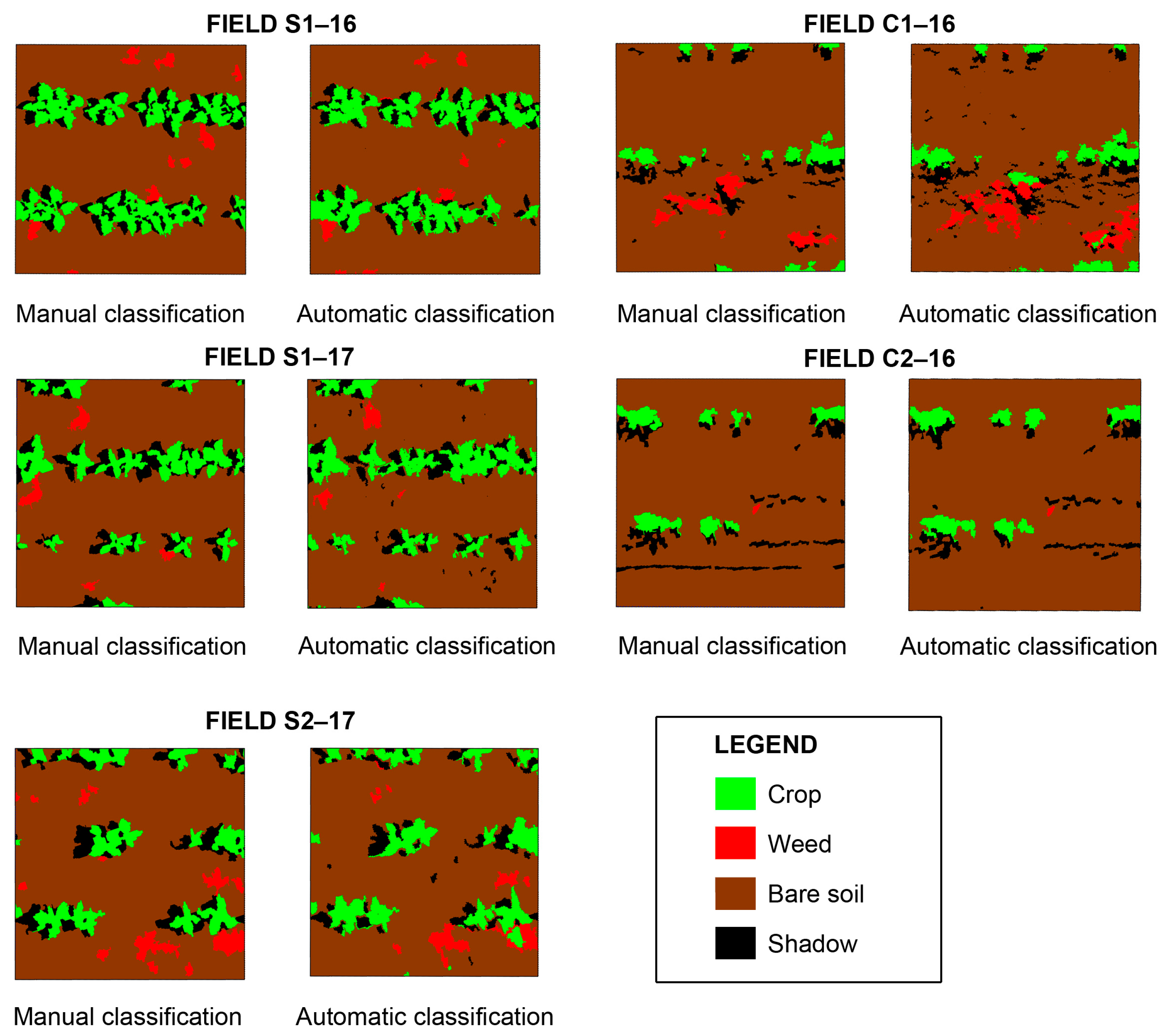
2.5. Weed Detection Validation

A set of 2 × 2 m squares placed in a 20 × 20 m grid was designed with the same orientation as the crop rows, using ArcGIS 10.0 (ESRI, Redlands, CA, USA) shapefiles to evaluate the performance of the weed classification algorithm. The number of validation frames for every field is shown in Table 1. The distribution of these sample frames was representative of the weed distribution in these fields.

Due to the low flight altitude (30 m), the mosaicked very high spatial resolution image made it possible to visually identify the individual plants in every reference frame, and thus conduct a manual digitization of the ground-truth data for crop plants, weeds and bare-soil in a shapefile (Figure 6). Thus, the on-ground weed infestation (manual weed coverage) was compared to the image classification process output (estimated weed coverage), and the accuracy was measured by calculating the slope and the coefficient of determination (R²) of the linear regression model.

In addition to the weed coverage (%), the weed density (weed plant/m²) was calculated from the classified map, since OBIA produces results that have both thematic and geometric properties [41]. Weed density is a crucial parameter for designing the herbicide application map [42]. However, there is limited research to provide suitable spatial accuracy measures for OBIA, and traditional accuracy assessment methods based upon site-specific reference data do not provide this kind of information [41]. To this end, an adequate accuracy index, called “Weed detection Accuracy” (WdA), following Equation (1), was designed to study the performance of every classified map. In this way, the classified OBIA outputs were evaluated both thematically and geometrically. Thus, the performance of weed cover was evaluated based on the linear regression model, and the WdA index assessed the spatial positioning of classified weeds. It did so by employing the intersection between both shapefiles as a better spatial relationship than the total overlap. This is because the manual object delineation of small weeds could be imprecise and subjective and not totally in agreement with the actual data. Thus, a weed was considered as correctly classified when it coincided with an observed weed, independently of edge coincidence.

$$\mathrm{WdA}(\%)=\frac{\mathrm{Area}\mathrm{of}\mathrm{Observed}\mathrm{Weed}\mathrm{objects}\mathrm{intersecting}\mathrm{Detected}\mathrm{Weed}\mathrm{Objects}}{\mathrm{Area}\mathrm{of}\mathrm{Observed}\mathrm{Weed}}\times 100$$

(1)

Thus, this approach overcomes some limitations of site-specific accuracy assessment methods typically associated with pixel-based classification when applied to object-based image analysis [41]. In addition, it could also answer the question suggested by Whiteside et al. [41] related to the thematic and geometrical typification accuracy of real world objects.

3. Results and Discussion

3.1. OBIA-Based Crop Height Estimations

Accuracy and graphical comparisons between the manually acquired and OBIA estimated crop heights by year, flight altitude and crop are shown in Figure 7. Most of the points were close to the 1:1 line, which indicated a high correlation among them. Moreover, very low RMSE values were achieved in all the case studies, all of them <0.04, showing an excellent fit of the OBIA-based model to the true data. The highest correlation (R² = 0.71) was achieved in sunflower at a 30 m flight altitude in 2016, being slightly lower for the rest of the case studies at the same flight height, maybe due to the higher plant height variability, This fact suggests that much better correlation could be reached when a wider crop height range is used.

Correlations obtained at the 60 m flight altitude were slightly worse than those reported at 30 m altitude because of the spatial resolution lost. Nevertheless, similar RSME magnitudes were observed between both approaches, independent of the flight altitude, which demonstrated algorithm robustness.

In the case of cotton, the algorithm indicated a tendency to overestimate the results, since most of the points were above the 1:1 line. This overestimation could be related to the land preparation, which consisted of small parallel channels created along the field for furrow irrigation (Figure 2). Thus, the OBIA algorithm calculated the plant height by selecting the surrounding on-ground baseline as the local minima, usually located in the furrow, and the plant apex as the local maxima. However, the cotton plants grow at the top of the ridge, and consequently, the height calculated by the algorithm took into account the height of the cotton plant as well as that of the ridge. Accordingly, this issue could be solved applying a height corrector related to the ridge height.

Additionally, the OBIA algorithm was able to identify every individual plant in the field and estimate the plant height feature of each one. The use of a DSM in the OBIA procedure enabled the efficient assessment of plant height, and the DSM creation was feasible due to the high overlap between UAV images. To the best of our knowledge, UAV photogrammetry has not yet been applied to estimate cotton and sunflower plant heights in early season, and subsequently, to validate the OBIA algorithm using ground truth data. Although a previous investigation used a similar image-based UAV technology to calculate cotton height [43], no field validation was performed, so this methodology remained non-validated at the early growth stage. In this context, some authors have estimated plant height at a late stage, such as Watanabe et al. [44], in barley fields just before harvest, and Varela et al. [45], some weeks before maize flowering, obtaining lower or similar R² values than our results: 0.52 and 0.63, respectively. Comparatively, the coefficient of correlation increased when the experiment was conducted at later stage, e.g., Varela et al. [45] achieved an R² of 0.79 in the abovementioned experiment, but used images taken at flowering stage, which denotes a positive relationship between both variables. Similarly, Iqbal et al. [9] achieved a stronger correlation (R² > 0.9) working in the late season with a broad range of poppy crop heights (0.5–0.9 m), and Bendig et al. [7] reported higher deviations from the regression line for younger plants. Therefore, the correlations obtained in this paper are considered very satisfactory, since the experiments were carried out in the challenging very early crop growth stage.

Plant height has been calculated in this experiment as a feature to avoid misclassification inside the crop row. However, through a combination with spectral vegetation indices, this geometric feature could be used for other purposes, such as crop phenotyping, biomass or yield estimation [10].

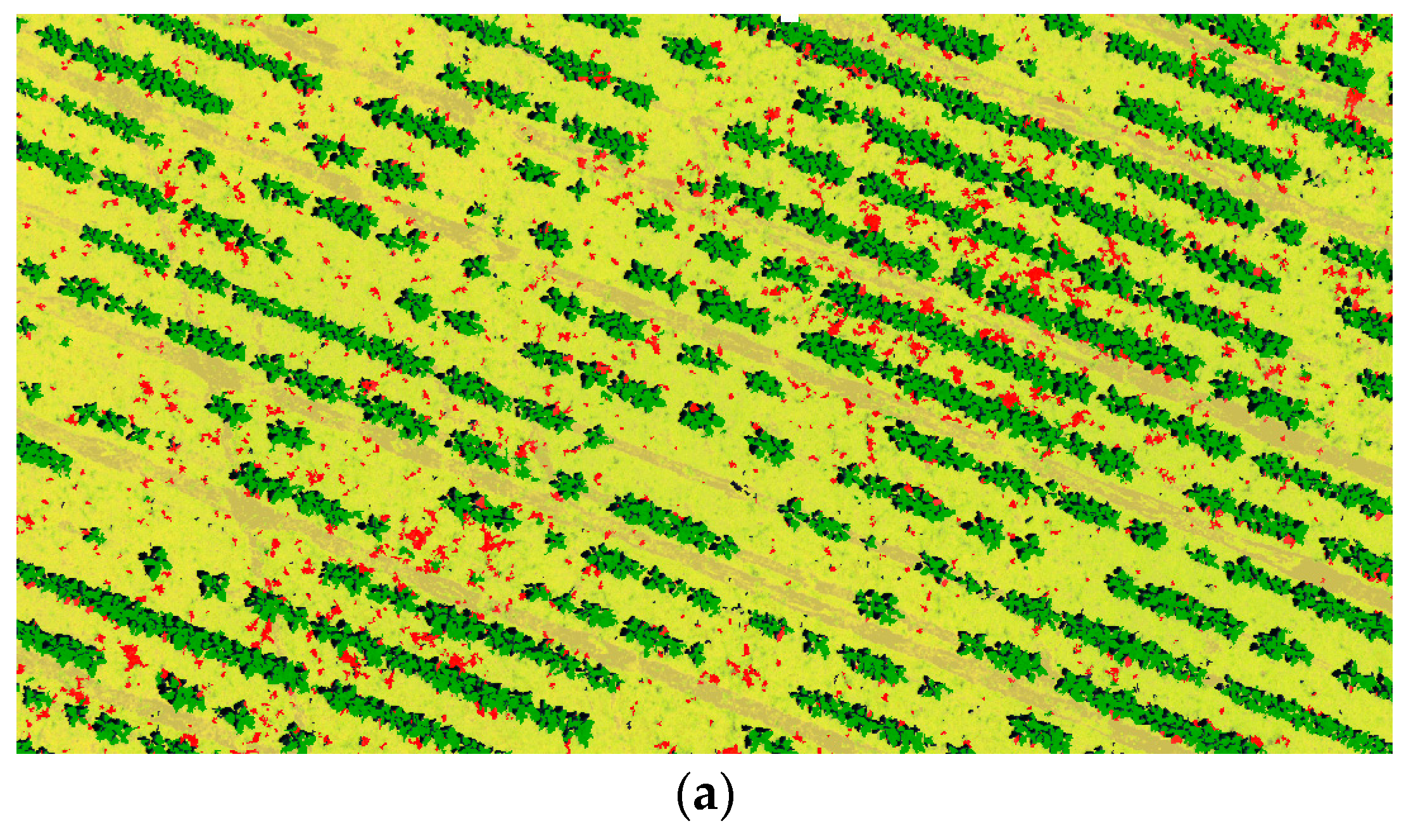
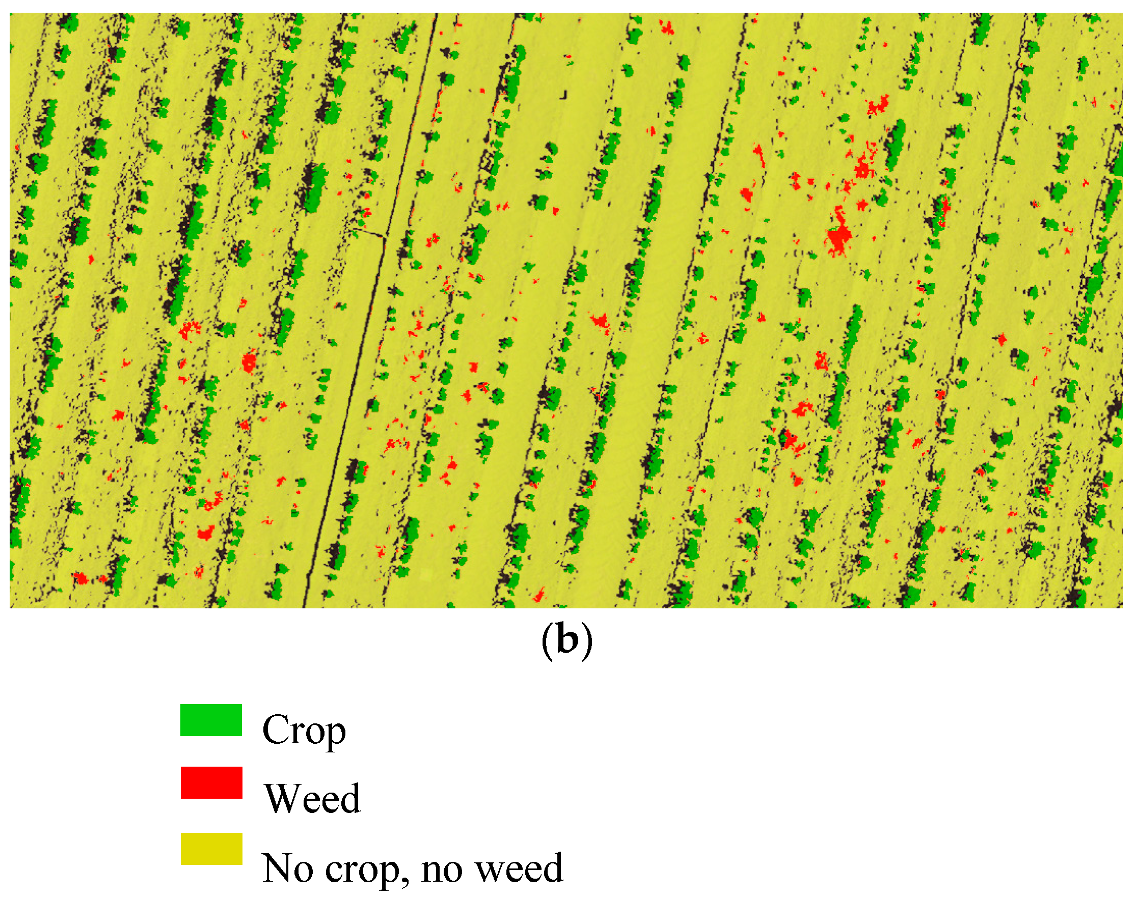
3.2. Automatic RF Training Set Selection and Classification

As a previous step of the training set selection, the crop rows were correctly identified. Then, the RF classifier randomly selected a training set for every class (

Table 2. Description of the training set automatically selected by the RF classifier implemented in the OBIA algorithm.

		Trainning Set Data
		Selected Training Objects (%) *				Selected Training Area over Total Field Area Φ
Field	Flight Altitude	Bare Soil	Crop	Shadow	Weed	Bare Soil	Crop	Shadow	Weed	Total
C1–16	30	23	28	27	22	1.0	0.9	0.7	0.5	3.0
C2–16	30	23	28	28	22	0.6	0.5	0.5	0.3	1.8
S1–16	30	19	28	30	23	1.4	1.1	1.1	0.8	4.2
	60	17	32	36	16	2.6	2.0	1.4	0.5	6.5
S1–17	30	21	28	29	23	1.5	1.3	1.2	0.9	4.9
	60	18	30	33	19	2.9	1.7	1.7	0.8	7.1
S2–17	30	20	28	29	23	1.4	1.4	1.4	1.0	5.2
	60	18	30	33	19	2.5	1.8	1.7	0.9	6.8

* selected training objects: percentage of objects selected for every class in the total training set data for the image. ^Φ selected training area over total field area (%): selected area as training data for every class over total image area.

). Sample selection was class balanced, as recommended by Belgiu and Drăguţ [17], through matching the object number to the least represented class, which was the weed class in most of the scenarios, e.g., in the C2–26 field, 23% of the data corresponded to bare soil objects, 28% to crop, 28% to shadow and 22% to weeds Thus, weed abundance in each field determined the percentage of objects selected for every class, as well as the full data set composition (second block in Table 2). The full data represented more than 0.25% of the total field area in all scenarios, as the minimum value recommended for training the RF algorithm [46]. For example, the full training data reached 4.2% in S1–16 at 30 m flight altitude, and the 6.8% in S2–16 for images taken at 60 m.

Despite being class balanced in terms of object numbers, bare soil tended to be the most represented class in terms of surface, because of the way MRS works by grouping areas of similar pixel values, resulting in larger objects for homogeneous classes (bare soil) and smaller objects for heterogeneous classes (vegetation), due to the small leaves composing the plants [34]. For example, bare soil represented a bigger training data surface (0.6%) compared to crop (0.5%) and weeds in the C2–16 field. These deviations in class balancing were higher for the images taken at 60 m due to the lower spatial resolution, which could generate a coarser delineation of plant objects. Accordingly, with the smaller vegetation sizes at the early growth stage, it would be more convenient to use images taken at 30 m with higher spatial resolution.

The automation of the RF training is an important asset that makes the classification process time-efficient, reliable and more accurate, removing errors from a subjective manual process. Moreover, this procedure is carried out in the same image that is going to be classified, which increases the classification accuracy [47].

3.3. Weed Detection

As a result of the RF training in every field image, an RF classifier was created, according to the automatically selected feature values in each image. The procedure was applied to different crops (cotton and sunflower) and flight heights (30 and 60 m). However, as anticipated in the previous section, due to the inferior results obtained by images taken at 60 m, only weed detection maps at the lowest flight altitude are shown [11] (Figure 8). Therefore, as a conclusion of this experiment, high spatial resolution is crucial for automatic weed mapping in early growth stages, which is feasible with a UAV.

A high level of agreement was reached in the comparison between the manual weed classification and that automatically performed by the RF-OBIA algorithm. Some examples of validation frames are shown in Figure 9. Sunflower plants are bigger than cotton, while the weed size was independent of the crop or date. The diversity of the study fields confirms the robustness of the procedure.

Correlation scatterplots and accuracy for comparisons are shown in Figure 10. The relationship between the estimated weed coverage from the UAV image classification, and the values observed in the on-ground sampling frames was satisfactory, with a coefficient of determination higher than 0.66 in most cases. This was the case for all fields, except for C1–16, indicating a good agreement for both crops. The worse fitting observed in this field was due to the small size and irregular shape of the leaves of many weeds that made it impossible to achieve a good manual delineation, overstating the actual weed infestation. However, for the sunflower scenarios there were points distributed all over the graphic. Thus, the correlation was closer to the 1:1 line in the sunflower fields, with an R² of 0.91 in both S1–17 and S2–17. These results were higher than those achieved by Peña et al. [11] (R² = 0.89) using a multispectral camera for early season maize detection. Thus, the use of the RF classifier as well as the plant height feature for sample selection enabled the improvement of weed coverage detection.

Table 3. Accuracy assessment on weed discrimination based on the Weed detection Accuracy (WdA) index attained for UAV images taken at 30 m flight altitude.

Crop	Field	WdA (%)
Cotton	C1–16	84.0
	C2–16	63.0
Sunflower	S1–16	59.1
	S1–17	87.9
	S2–17	81.1

shows the spatial accuracy measures obtained by the WdA index. WdA results varied according to the image and crop. High WdA values were found in most of the classified maps, indicating that majority of weeds were correctly identified and located, e.g., 84% of weeds in the cotton field (C1–16) and 81.1% in sunflower (S2–17). Table 3 shows the spatial accuracy measures obtained by the WdA index. WdA results varied according to the image and crop. High WdA values were found in most of the classified maps, indicating that majority of weeds were correctly identified and spatially located, e.g., 84% of weeds in the cotton field (C1–16) and 81.1% in the sunflower field (S2–17). We consider that the criteria for successful classification is an 80% minimum WdA (based on previous studies), which was achieved in C1–16, S1–17 and S2–17. The precision value requirement may be considered to be 60% when mapping complex vegetation classifications [48], and mapping weed within rows in the early growth stage is considered one of the main challenges facing agricultural researchers [5]. In this experiment, an spatial accuracy more than 60% was achieved in all the classified map, with the exception of S1–16, where a close value was obtained (59.1%). The poor results reached in S1–16 could be explained by the smaller plant sizes due to developmental delay, which makes the discrimination from bare soil more complicated. Thus, different weed coverage is present in different growth stages affecting the weed discrimination process. The best results were achieved in S1–17 and S2–17 sunflower fields, with R² values of 0.91, indicating an accurate definition of the weed shape and edge, and WdA values of 87.9% and 81.1%, respectively, which indicated that the algorithm was able to locate most of the weeds.

Both measures provide general and spatial classification accuracy, i.e., proved that the algorithm properly identified, delineate the edge and quantify the surface of every weed. In cotton, the algorithm provided a lower quality in weed estimation (R² = 0.57), with most values located above the 1:1 line, indicating overestimation of the weed infestation. From an agronomical perspective, overestimation is not a problem, because it reduces the chance of missing weeds, rather than taking the risk of allowing weeds to go untreated [49].

In general, accurate weed classification results were obtained in both crops using high spatial resolution images. Weed abundance and consequently, the training data set were key factors in the accuracy of the classification. A very high capacity to classify weeds was obtained using an image surface value higher than 0.8% as a weed training data set. Therefore, according to our results, the automatic RF-OBIA procedure is able to classify weeds between and within the crop rows at an early growth stage, considering the variety of situations evaluated in this study.

3.4. Prescription Maps

The OBIA algorithm automatically created the prescription maps based on the weed maps (Figure 11). The correctness of the prescription maps strongly depends on the accuracy of the weed maps, and, consequently, will define the efficiency of site-specific weed management (SSWM) [2]. Implementing SSWM requires locating weeds at densities greater than those that would cause economic losses [50]. Nevertheless, in this study, prescription maps were generated by using the presence of weeds as a weed treatment threshold, which determines the weed infestation level above which a treatment is required [42]. That is, in our experiment, conservative prescription maps, from which the minimum herbicide savings occur, were generated, since any grid with a number of weeds equal to or higher than 1 was considered a treatment area, independently of weed size. This parameter is customizable and can be adapted to other agronomical scenarios, noting that, when a less restrictive weed treatment threshold is selected, higher herbicide reduction and consequent benefits can be achieved.

The potential herbicide savings based on those prescription maps are shown in

Table 4. Herbicide savings obtained from herbicide application maps based on treatment threshold of 0%.

Crop	Field	Herbicide Saving (%)
Cotton	C1–16	60
	C2–16	79
Sunflower	S1–16	27
	S1–17	37
	S2–17	28

. The percentages of savings depend on weed distribution within the field, and, consequently, vary across the five fields. The highest percentages were shown in areas with low levels of weed infestation, e.g., the 60% and 79% of herbicide savings for cotton C1–16 and C2–16, respectively. Moreover, due to the higher level of infestation, lower herbicide savings were obtained in the sunflower field (Figure 10). Thus, the saving in herbicide, calculated in terms of untreated areas, ranged from 27% to 79%, compared to a conventional uniform blanket application. In addition to this relevant reduction of the use of herbicides, the use of a prescription map would lead farmers to optimize fuel, field operating time and cost.

The optimization of weed management practices relies on timing weed control [51], as weed presence in the early crop season is a key component of the weed-crop competition and further yield loss [52,53]. Thus, it is essential to maintain a weed-controlled environment for the crop at these initial growth stages [54], making quick weed detection a crucial tool for preventing yield losses. On the other hand, the timing of post-emergency herbicide applications impacts control efficiency [55]. Usually, the herbicide application window depends on weather conditions, weed species and crops, and can be as short as a two- to three-day window. Although some researchers have achieved interesting results in terms of weed detection and herbicide savings based on on-the-go weed detection systems and field surveys [56,57,58], they are time consuming and costly. It could delay the herbicide application that may reduce herbicide effectiveness [59]. The time involved in the entire process (acquisition and mosaicking the images, and running the algorithm) in our experiment took less than 40 h per field. Therefore, by using UAV-images in combination with the developed RF-OBIA algorithm, herbicide treatment in the early crop season could be applied as quickly as two days after a farmer requests a herbicide application or weed infestation map.

Information generated in this paper includes three key components of a successful SSWM system: weed map (location, number and coverage of weed); prescription map (user-configurable); and timely information, i.e., both maps are provided at the critical period for weed control. Thereby, farmers may design a proper and timely weed-management strategy [53]—the density, size and coverage of weed are associated with the appropriate application time (critical period), herbicide control efficacy [60,61] and economical herbicide threshold [50].

Consequently, the technological combination of UAV imagery and the RF-OBIA algorithm developed will enable rapid, timely and accurate mapping of weeds to design the application map for early season crops. The use of these early maps could help farmers in SSWM decision-making, providing guidelines for early post-emergence herbicide application, in order to optimize crop management, reduce yield losses, rationalize herbicide application, and save time and costs. Additionally, it would achieve the basic premise relative to the timing of weed management—good weed management should be judged on decisions made early in the development of the crop, not on appearance at harvest.

4. Conclusions

Based on the importance of having timely and accurate weed maps in early season crops for proper weed management, an innovative automatic RF-OBIA algorithm to create early season post-emergence SSWM maps was developed for herbaceous crops. DSMs, from 3D models, and orthomosaics, generated from RGNIR-images and machine learning techniques (RF), were combined in the OBIA algorithm, to self-train, select feature values and classify weeds, between and within crop rows. First, the OBIA algorithm identified every individual plant (including weeds and crop) in the image and accurately estimated its plant height feature based on the DSM. Better results were achieved for sunflower plants in terms of height estimation, while cotton plant heights tended to be slightly overestimated, probably caused by the land preparation for furrow irrigation. Second, the RF classifier randomly selected a class balanced training set in each image, without requiring an exhaustive training process, which allowed the optimum feature values for weed mapping to be chosen. This automatic process is an important asset that makes this procedure time-efficient, reliable and more accurate, since it removes errors from a subjective manual process. In this way, the RF-OBIA method offered a significant improvement compared to conventional classifiers. The system’s ability to detect the smallest weeds was impaired in images with lower spatial resolution, showing the necessity of 0.6 cm of pixel size for reliable detection, feasible in the UAV mission. Furthermore, weed abundance and weed spatial distribution could also be calculated by the algorithm. Thirdly, useful prescription maps for in season post-emergence SSWM were created based on the weed maps. In addition, the short time (less than 40 h per field) involved in the entire process (image capture, mosaicking and analysis) allows timely weed control during the critical period, which is crucial for preventing weed–crop competition and future yield losses.

Alternatively, machine vision systems have shown potential for agricultural tasks [62,63], and some research studies have used these techniques to detect and identify plant species (either crops or weeds) [58,64,65]. Therefore, a comparison between tractor-mounted sensors and OBIA-UAV technology must be conducted in further research.

In summary, the combination of UAV imagery and RF-OBIA developed in this paper will enable rapid and accurate weed mapping, between and within crop rows, to design herbicide application in the early season, which could help farmers in the decision-making process, providing guidelines for site-specific post-emergence herbicide application, in order to optimize crop management, reduce yield loss, rationalize herbicide application and, consequently, save time and reduce costs. Additionally, this critical information can be provided quickly, during the most critical period for weed control, achieving one other key premise for weed management.

References

1. Peña, J.M.; Torres-Sánchez, J.; Serrano-Pérez, A.; de Castro, A.I.; López-Granados, F. Quantifying efficacy and limits of unmanned aerial vehicle (UAV) technology for weed seedling detection as affected by sensor resolution. Sensors 2015, 15, 5609–5626. [Google Scholar] [CrossRef] [PubMed]
2. Castaldi, F.; Pelosi, F.; Pascucci, S.; Casa, R. Assessing the potential of images from unmanned aerial vehicles (UAV) to support herbicide patch spraying in maize. Precis. Agric. 2017, 18, 76–94. [Google Scholar] [CrossRef]
3. Pérez-Ortiz, M.; Peña, J.M.; Gutiérrez, P.A.; Torres-Sánchez, J.; Hervás-Martínez, C.; López-Granados, F. A semi-supervised system for weed mapping in sunflower crops using unmanned aerial vehicles and a crop row detection method. Appl. Soft Comput. 2015, 37, 533–544. [Google Scholar] [CrossRef]
4. López-Granados, F. Weed detection for site-specific weed management: Mapping and real-time approaches. Weed Res. 2011, 51, 1–11. [Google Scholar] [CrossRef]
5. López-Granados, F.; Torres-Sánchez, J.; de Castro, A.I.; Serrano-Pérez, A.; Mesas-Carrascosa, F.J.; Peña, J.M. Object-based early monitoring of a grass weed in a grass crop using high resolution UAV imagery. Agron. Sustain. Dev. 2016, 36, 67. [Google Scholar] [CrossRef]
6. Nex, F.; Remondino, F. UAV for 3D mapping applications: A review. Appl. Geomat. 2013, 6, 1–15. [Google Scholar] [CrossRef]
7. Bendig, J.; Bolten, A.; Bennertz, S.; Broscheit, J.; Eichfuss, S.; Bareth, G. Estimating biomass of barley using crop surface models (CSMs) derived from UAV-based RGB imaging. Remote Sens. 2014, 6, 10395–10412. [Google Scholar] [CrossRef]
8. Geipel, J.; Link, J.; Claupein, W. Combined spectral and spatial modeling of corn yield based on aerial images and crop surface models acquired with an unmanned aircraft system. Remote Sens. 2014, 6, 10335. [Google Scholar] [CrossRef]
9. Iqbal, F.; Lucieer, A.; Barry, K.; Wells, R. Poppy crop height and capsule volume estimation from a single UAS flight. Remote Sens. 2017, 9, 647. [Google Scholar] [CrossRef]
10. Ostos, F.; de Castro, A.I.; Pistón, F.; Torres-Sánchez, J.; Peña, J.M. High-throughput phenotyping of bioethanol potential in cereals by using multi-temporal UAV-based imagery. Front. Plant Sci. 2018. under review. [Google Scholar]
11. Peña, J.M.; Torres-Sánchez, J.; de Castro, A.I.; Kelly, M.; López-Granados, F. Weed mapping in early-season maize fields using object-based analysis of unmanned aerial vehicle (UAV) images. PLoS ONE 2013, 8, e77151. [Google Scholar] [CrossRef] [PubMed]
12. Blaschke, T.; Hay, G.J.; Kelly, M.; Lang, S.; Hofmann, P.; Addink, E.; Queiroz Feitosa, R.; van der Meer, F.; van der Werff, H.; van Coillie, F.; et al. Geographic object-based image analysis—Towards a new paradigm. ISPRS J. Photogramm. Remote Sens. 2014, 87, 180–191. [Google Scholar] [CrossRef] [PubMed]
13. López-Granados, F.; Torres-Sánchez, J.; Serrano-Pérez, A.; de Castro, A.I.; Mesas-Carrascosa, F.J.; Peña, J.M. Early season weed mapping in sunflower using UAV technology: Variability of herbicide treatment maps against weed thresholds. Precis. Agric. 2016, 17, 183–199. [Google Scholar] [CrossRef]
14. Pérez-Ortiz, M.; Peña, J.M.; Gutiérrez, P.A.; Torres-Sánchez, J.; Hervás-Martínez, C.; López-Granados, F. Selecting patterns and features for between- and within- crop-row weed mapping using UAV-imagery. Expert Syst. Appl. 2016, 47, 85–94. [Google Scholar] [CrossRef]
15. Ghimire, B.; Rogan, J.; Galiano, V.R.; Panday, P.; Neeti, N. An evaluation of bagging, boosting, and random forests for land-cover classification in cape cod, Massachusetts, USA. GISci. Remote Sens. 2012, 49, 623–643. [Google Scholar] [CrossRef]
16. Rodriguez-Galiano, V.F.; Ghimire, B.; Rogan, J.; Chica-Olmo, M.; Rigol-Sanchez, J.P. An assessment of the effectiveness of a random forest classifier for land-cover classification. ISPRS J. Photogramm. Remote Sens. 2012, 67, 93–104. [Google Scholar] [CrossRef]
17. Belgiu, M.; Drăguţ, L. Random forest in remote sensing: A review of applications and future directions. ISPRS J. Photogramm. Remote Sens. 2016, 114, 24–31. [Google Scholar] [CrossRef]
18. Du, P.; Samat, A.; Waske, B.; Liu, S.; Li, Z. Random forest and rotation forest for fully polarized SAR image classification using polarimetric and spatial features. ISPRS J. Photogramm. Remote Sens. 2015, 105, 38–53. [Google Scholar] [CrossRef]
19. Ho, T.K. Random Decision Forests. In Proceedings of the 3rd International Conference on Document Analysis and Recognition, Montreal, QC, Canada, 14–16 August 1995; pp. 278–282. [Google Scholar]
20. Breiman, L. Random Forests. Mach. Learn. 2001, 45, 5–32. [Google Scholar] [CrossRef]
21. Li, M.; Ma, L.; Blaschke, T.; Cheng, L.; Tiede, D. A systematic comparison of different object-based classification techniques using high spatial resolution imagery in agricultural environments. Int. J. Appl. Earth Obs. 2016, 49, 87–98. [Google Scholar] [CrossRef]
22. Chan, J.C.W.; Beckers, P.; Spanhove, T.; Borre, J.V. An evaluation of ensemble classifiers for mapping Natura 2000 heathland in Belgium using spaceborne angular hyperspectral (CHRIS/Proba) imagery. Int. J. Appl. Earth Obs. 2012, 18, 13–22. [Google Scholar] [CrossRef]
23. Foody, G.M. Thematic map comparison: Evaluating the statistical significance of differences in classification accuracy. Photogramm. Eng. Remote Sens. 2004, 70, 627–633. [Google Scholar] [CrossRef]
24. Pal, M. Random forest classifier for remote sensing classification. Int. J. Remote Sens. 2005, 26, 217–222. [Google Scholar] [CrossRef]
25. Lottes, P.; Khanna, R.; Pfeifer, J.; Siegwart, R.; Stachniss, C. UAV-based crop and weed classification for smart farming. In Proceedings of the IEEE International Conference on Robotics and Automation (ICRA), Singapore, 29 May–3 June 2017; pp. 3024–3031. [Google Scholar]
26. Ma, L.; Cheng, L.; Li, M.; Liu, Y.; Ma, X. Training set size, scale, and features in Geographic Object-based image analysis of very high resolution unmanned aerial vehicle imagery. ISPRS J. Photogramm. Remote Sens. 2015, 102, 14–27. [Google Scholar] [CrossRef]
27. Meier, U. BBCH Monograph: Growth Stages for Mono- and Dicotyledonous Plants, 2nd ed.; Blackwell Wiss.-Verlag: Berlin, German, 2001. [Google Scholar] [CrossRef]
28. Torres-Sánchez, J.; López-Granados, F.; Serrano, N.; Arquero, O.; Peña, J.M. High-throughput 3-D monitoring of agricultural-tree plantations with unmanned aerial vehicle (UAV) Technology. PLoS ONE 2015, 10, e0130479. [Google Scholar] [CrossRef] [PubMed]
29. AESA. Aerial Work—Legal Framework. Available online: http://www.seguridadaerea.gob.es/LANG_EN/cias_empresas/trabajos/rpas/marco/default.aspx (accessed on 13 December 2017).
30. Dandois, J.P.; Ellis, E.C. High spatial resolution three-dimensional mapping of vegetation spectral dynamics using computer vision. Remote Sens. Environ. 2013, 136, 259–276. [Google Scholar] [CrossRef]
31. Baatz, M.; Schäpe, A. Multiresolution Segmentation: An Optimization Approach for High Quality Multi-Scale Image Segmentation. 2000. Available online: http://www.ecognition.com/sites/default/files/405_baatz_fp_12.pdf (accessed on 6 November 2017).
32. Drăguţ, L.; Csillik, O.; Eisank, C.; Tiede, D. Automated parameterisation for multi-scale image segmentation on multiple layers. ISPRS J. Photogramm. Remote Sens. 2014, 88, 119–127. [Google Scholar] [CrossRef] [PubMed]
33. Torres-Sánchez, J.; López-Granados, F.; Peña, J.M. An automatic object-based method for optimal thresholding in UAV images: Application for vegetation detection in herbaceous crops. Comput. Electron. Agric. 2015, 114, 43–52. [Google Scholar] [CrossRef]
34. eCognition. Definiens Developer 9.2: Reference Book; Definiens AG: Munich, German, 2016. [Google Scholar]
35. De Castro, I.A.; Ehsani, R.; Ploetz, R.; Crane, J.H.; Abdulridha, J. Optimum spectral and geometric parameters for early detection of laurel wilt disease in avocado. Remote Sens. Environ. 2015, 171, 33–44. [Google Scholar] [CrossRef]
36. Peña, J.M.; López-Granados, F.; Jurado-Expósito, M.; García-Torres, L. Mapping Ridolfia segetum patches in sunflower crop using remote sensing. Weed Res. 2007, 47, 164–172. [Google Scholar] [CrossRef]
37. Otsu, N. A Threshold Selection Method from Gray-Level Histograms. IEEE Trans. Syst. Man Cybern. 1979, 9, 62–66. [Google Scholar] [CrossRef]
38. Peña, J.M.; Kelly, M.; de Castro, A.I.; López-Granados, F. Object-based approach for crow row characterization in UAV images for site-specific weed management. In Proceedings of the 4th International Conference on Geographic Object-Based Image Analysis (GEOBIA), Rio de Janeiro, Brazil, 7–9 May 2012; pp. 426–430. [Google Scholar]
39. Williams, G.J. Rattle: A data mining GUI for R. R. J. 2009, 1, 45–55. [Google Scholar]
40. Gonzalez-de-Santos, P.; Ribeiro, A.; Fernandez-Quintanilla, C.; Lopez-Granados, F.; Brandstoetter, M.; Tomic, S.; Pedrazzi, S.; Peruzzi, A.; Pajares, G.; Kaplanis, G.; et al. Fleets of robots for environmentally-safe pest control in agriculture. Precis. Agric. 2017, 18, 574–614. [Google Scholar] [CrossRef]
41. Whitside, T.G.; Maier, S.F.; Boggs, G.S. Area-based and location-based validation of classified image objects. Int. J. Appl. Earth Obs. Geoinform. 2014, 28, 117–130. [Google Scholar] [CrossRef]
42. Longchamps, L.; Panneton, B.; Simard, M.J.; Leroux, G.D. An imagery-based weed cover threshold established using expert knowledge. Weed Sci. 2014, 62, 177–185. [Google Scholar] [CrossRef]
43. Chu, T.; Chen, R.; Landivar, J.A.; Maeda, M.M.; Yang, C.; Starek, M.J. Cotton growth modeling and assessment using unmanned aircraft system visual-band imagery. J. Appl. Remote Sens. 2016, 10, 036018. [Google Scholar] [CrossRef]
44. Watanabe, K.; Guo, W.; Arai, K.; Takanashi, H.; Kajiya-Kanegae, H.; Kobayashi, M.; Yano, K.; Tokunaga, T.; Fujiwara, T.; Tsutsumi, N.; et al. High-throughput phenotyping of sorghum plant height using an unmanned aerial vehicle and its application to genomic prediction modeling. Front. Plant Sci. 2017, 8, 421. [Google Scholar] [CrossRef] [PubMed]
45. Varela, S.; Assefa, Y.; Prasad, P.V.V.; Peralta, N.R.; Griffin, T.W.; Sharda, A.; Ferguson, A.; Ciampitti, I.A. Spatio-temporal evaluation of plant height in corn via unmanned aerial systems. J. Appl. Remote Sens. 2017, 11, 036013. [Google Scholar] [CrossRef]
46. Colditz, R.R. An evaluation of different training sample allocation schemes for discrete and continuous land cover classification using decision tree-based algorithms. Remote Sens. 2015, 7, 9655–9681. [Google Scholar] [CrossRef]
47. Vetrivel, A.; Gerke, M.; Kerle, N.; Vosselman, G. Identification of damage in buildings based on gaps in 3D point clouds from very high resolution oblique airborne images. ISPRS J. Photogramm. Remote Sens. 2015, 105, 61–78. [Google Scholar] [CrossRef]
48. Yu, Q.; Gong, P.; Clinton, N.; Biging, G.; Kelly, M.; Schirokauer, D. Classification with airborne high spatial resolution remote sensing imagery. Photogramm. Eng. Remote Sens. 2006, 72, 799–811. [Google Scholar] [CrossRef]
49. Gibson, K.D.; Dirk, R.; Medlin, C.R.; Johnston, L. Detection of weed species in soybean using multispectral digital images. Weed Technol. 2004, 18, 742–749. [Google Scholar] [CrossRef]
50. De Castro, A.I.; López Granados, F.; Jurado-Expósito, M. Broad-scale cruciferous weed patch classification in winter wheat using QuickBird imagery for in-season site-specific control. Precis. Agric. 2013, 14, 392–413. [Google Scholar] [CrossRef]
51. Pages, E.R.; Cerrudo, D.; Westra, P.; Loux, M.; Smith, K.; Foresman, C.; Wright, H.; Swanton, C.J. Why early season weed control is important in maize. Weed Sci. 2014, 60, 423–430. [Google Scholar] [CrossRef]
52. O’Donovan, J.T.; de St. Remy, E.A.; O’Sullivan, P.A.; Dew, D.A.; Sharma, A.K. Influence of the relative time of emergence of wild oat (Avena fatua) on yield loss of barley (Hordeum vulgare) and wheat (Triticum aestivum). Weed Sci. 1985, 33, 498–503. [Google Scholar] [CrossRef]
53. Swanton, C.J.; Mahoney, K.J.; Chandler, K.; Gulden, R.H. Integrated weed management: Knowledge based weed management systems. Weed Sci. 2008, 56, 168–172. [Google Scholar] [CrossRef]
54. Knezevic, S.Z.; Evans, S.P.; Blankenship, E.E.; Acker, R.C.V.; Lindquist, J.L. Critical period for weed control: The concept and data analysis. Weed Sci. 2002, 50, 773–786. [Google Scholar] [CrossRef]
55. Judge, C.A.; Neal, J.C.; Derr, J.F. Response of Japanese Stiltgrass (Microstegium vimineum) to Application Timing, Rate, and Frequency of Postemergence Herbicides. Weed Technol. 2005, 19, 912–917. [Google Scholar] [CrossRef]
56. Wiles, L.J. Beyond patch spraying: Site-specific weed management with several herbicides. Precis. Agric. 2009, 10, 277–290. [Google Scholar] [CrossRef]
57. Hamouz, P.; Hamouzová, K.; Holec, J.; Tyšer, L. Impact of site-specific weed management on herbicide savings and winter wheat yield. Plant Soil Environ. 2013, 59, 101–107. [Google Scholar] [CrossRef]
58. Gerhards, R.; Oebel, H. Practical experiences with a system for site-specific weed control in arable crops using real-time image analysis and GPS-controlled patch spraying. Weed Res. 2006, 46, 185–193. [Google Scholar] [CrossRef]
59. Chauhan, B.S.; Singh, R.G.; Mahajan, G. Ecology and management of weeds under conservation agriculture: A review. Crop Prot. 2012, 38, 57–65. [Google Scholar] [CrossRef]
60. Dunan, C.M.; Westra, P.; Schweizer, E.E.; Lybecker, D.W.; Moore, F.D., III. The concept and application of early economic period threshold: The case of DCPA in onions (Allium cepa). Weed Sci. 1995, 43, 634–639. [Google Scholar]
61. Weaver, S.E.; Kropff, M.J.; Groeneveld, R.M.W. Use of ecophysiological models for crop—Weed interference: The critical period of weed interference. Weed Sci. 1992, 40, 302–307. [Google Scholar] [CrossRef]
62. García-Santillan, I.; Pajares, G. On-line crop/weed discrimination through the Mahalanobis distance from images in maize fields. Biosyst. Eng. 2018, 166, 28–43. [Google Scholar] [CrossRef]
63. Barreda, J.; Ruíz, A.; Ribeiro, A. Seguimiento Visual de Líneas de Cultivo (Visual Tracking of Crop Rows). Master’s Thesis, Universidad de Murcia, Murcia, Spain, 2009. [Google Scholar]
64. Slaughter, D.C.; Giles, D.K.; Downey, D. Autonomous robotic weed control systems: A review. Comput. Electron. Agric. 2008, 61, 63–78. [Google Scholar] [CrossRef]
65. Andújar, D.; Escola, A.; Dorado, J.; Fernandez-Quintanilla, C. Weed discrimination using ultrasonic sensors. Weed Res. 2011, 51, 543–547. [Google Scholar] [CrossRef]
Figure 1. General view of the three studied sunflower crops in early stage: (a) S1–16; (b) S1–17; (c) S1–17.
Remotesensing 10 00285 g001
Figure 2. General view of the two studied cotton crops in the early stage: (a) C1–16, (b) C2–16.
Remotesensing 10 00285 g002
Figure 3. (a) Detail of one of the studied sunflower fields; (b) A partial view of the corresponding DSM produced by the photogrammetric processing of the remote images taken with the UAV.
Remotesensing 10 00285 g003
Figure 4. Flowchart and graphical examples of the Object Based Image Analysis (OBIA) procedure outputs for weed detection outside and within crop rows.
Remotesensing 10 00285 g004
Figure 5. Field work images depicting: (a) acquisition of GPS coordinates of validation points; (b) measurement of the plant height.
Remotesensing 10 00285 g005
Figure 6. Detail of a validation frames in field S1–16: (a) original image (G-NIR-R composition); (b) manually classified frame.
Remotesensing 10 00285 g006
Figure 7. OBIA-based estimated height vs. observed height as affected by crop, fight altitude and year. The root mean square error (RMSE) and correlation coefficient (R2) derived from the regression fit are included for every scenario (p < 0.0001). The solid line is the fitted linear function and the red dotted line is the 1:1 line.
Remotesensing 10 00285 g007
Figure 8. Classified image by applying the auto-trained Random Forest classifier Object Based Image Analysis (RF-OBIA) algorithm to Unmanned Aerial Vehicle (UAV) images at 30 m flight altitude: (a) sunflower field; (b) cotton field.
Remotesensing 10 00285 g008aRemotesensing 10 00285 g008b
Figure 9. Examples of 2 × 2 frames validation frames, showing manual and automatic OBIA-based classification from each studied field image, taken at 30 m flight altitude.
Remotesensing 10 00285 g009
Figure 10. Graphics comparing observed and OBIA-estimated weed coverage at the 30 m flight altitude: (a) cotton fields; (b) sunflower fields. Correlation coefficients (R2) derived from the calculated regression fit are included for every scenario (p < 0.0001). The solid and dotted lines represent the fitted linear function and the 1:1 line, respectively.
Remotesensing 10 00285 g010
Figure 11. Prescription maps based on a treatment threshold of 0% obtained in: (a) sunflower; (b) cotton. Reference system UTM 30N, datum ETRS-89.
Remotesensing 10 00285 g011