Using Support Vector Regression and Hyperspectral Imaging for the Prediction of Oenological Parameters on Different Vintages and Varieties of Wine Grape Berries

Abstract

The performance of a support vector regression (SVR) model with a Gaussian radial basis kernel to predict anthocyanin concentration, pH index and sugar content in whole grape berries, using spectroscopic measurements obtained in reflectance mode, was evaluated. Each sample contained a small number of whole berries and the spectrum of each sample was collected during ripening using hyperspectral imaging in the range of 380–1028 nm. Touriga Franca (TF) variety samples were collected for the 2012–2015 vintages, and Touriga Nacional (TN) and Tinta Barroca (TB) variety samples were collected for the 2013 vintage. These TF vintages were independently used to train, validate and test the SVR methodology; different combinations of TF vintages were used to train and test each model to assess the performance differences under wider and more variable datasets; the varieties that were not employed in the model training and validation (TB and TN) were used to test the generalization ability of the SVR approach. Each case was tested using an external independent set (with data not included in the model training or validation steps). The best R² results obtained with varieties and vintages not employed in the model’s training step were 0.89, 0.81 and 0.90, with RMSE values of 35.6 mg·L⁻¹, 0.25 and 3.19 °Brix, for anthocyanin concentration, pH index and sugar content, respectively. The present results indicate a good overall performance for all cases, improving the state-of-the-art results for external test sets, and suggesting that a robust model, with a generalization capacity over different varieties and harvest years may be obtainable without further training, which makes this a very competitive approach when compared to the models from other authors, since it makes the problem significantly simpler and more cost-effective.

1. Introduction

As increases in computational power and processing capability continue, the introduction of new technologies into the most diverse industry segments is expanding, viticulture and the whole wine industry being no exception. With producers and companies demanding cheaper and faster ways to produce higher-quality wine from their vineyards, together with the massive increases in information available to the market, the search for a competitive advantage is increasing. One such advantage can be found in the development of new methodologies to reduce the cost of gathering information about grapes in an environmentally-friendly and timely manner, allowing winemakers to obtain more frequent insights into their wine grapes, to enable harvesting them at the optimal point of maturity and selecting them according to certain quality features.

Laboratory-based hyperspectral imaging collects information on how objects reflect and absorb light as a function of wavelength, providing both spatial and spectral information [1,2]. The main advantage of this kind of image-based system in comparison with traditional chemical analysis is that it is non-destructive and reduces the overall cost of the acquisition of quality information. However, it involves complex data that requires powerful analysis tools to extract the necessary information from the underlying patterns in the spectra. In recent years, the use of hyperspectral techniques combined with proper data analysis tools for extracting information has become an important technique to measure different oenological parameters that are highly involved in the evaluation of grapes’ ripeness stage. The most commonly used equipment in the literature operates simultaneously in the visible and near-infrared range, between 400–1000 nm, although the near-infrared wavelength above 1000 nm may contain important absorption bands. A possible reason for the extensive use of that range, in addition to the good results obtained, may be related to the fact that equipment operating at larger wavelengths tends to be significantly more expensive.

In this process of analysis and evaluation, the sugar content, anthocyanin concentration and pH index are highly researched parameters because they are correlated with the flavour, colour and are good indicators of the grapes’ ripeness. At this stage of the maturation process the level of anthocyanin and sugars increases, while the acidity diminishes sharply, leaving a signature in the spectral activity of the grapes. Nevertheless, due to several factors such as different climate changes, soil quality, sun exposition, water assessment, altitude and harvest time, a large variability may be present in the vineyards and consequently in the quality of the grapes and in the profile of the different oenological parameters. In recent years, the use of hyperspectral image-based methods for the prediction of such parameters has been proposed, using (a) transmittance mode [3,4], (b) interactance mode [5,6,7], and (c) reflectance mode. Since for the same illumination scenario the intensity of light reflected from the grape is stronger, which facilitates measurements, we chose reflectance mode spectroscopy for our methodology, making it more relevant to analysing previous results in the reflectance mode. The works on the reflectance mode can be further divided into (1) the reflectance mode for a small number of berries in each sample [8,9,10,11,12,13,14,15,16], using partial least squares (PLS), neural networks (NN) and least-squares support vector machines (LSSVM); and (2) reflectance mode for a large number of berries in each sample [17,18,19,20,21,22,23,24,25], using PLS or modified partial least squares (MPLS). Using a small number of berries per sample comprises a more difficult problem, since the samples’ variability is higher than when using samples with a larger number of berries, where the reference measurements result from the mixture of the individual berries.

The use and effectiveness of support vector machines combined with hyperspectral imaging ([26]) has already been tested and widely employed in classification problems [27,28,29], but approaches using regression are still uncommon. Other works are available that measure different chemical compounds (for example, phenolic compounds, solid sugar compounds or aroma compounds) [30,31,32,33,34].

Table 1. Literature results for the prediction of the oenological parameters for whole wine grape berries with hyperspectral imaging performed in reflectance mode.

		External Test Set
Oenological Parameter	Author	R2	RMSE
Sugar Content	Arana et al. [8]	0.710	1.270 °Brix
	Cao et al. [9]	0.820 4	0.960 °Brix 4
	Fadock et al. [19] 1,3	0.710	0.870 °Brix
	Fadock et al. [19] 3	0.910	0.650 °Brix
	Fernandes et al. [10]	0.920	0.950 °Brix
	Gomes et al. [13]	0.959	1.026 °Brix
	Gomes et al. [12]	0.948	0.939 °Brix
	Gomes et al. [15] 1	0.948	1.344 °Brix
	González-Caballero et al. [21] 3	0.910 4	1.000 °Brix 4
	Nogales-Bueno et al. [25] 3	0.990 4	1.370 °Brix 4
	Wu et al. [16]	0.908	4
pH Values	Cao et al. [9]	0.957 4	0.126 4
	Cozzolino et al. [18] 3	0.850 4	0.150 4
	Fadock et al. [19] 1,3	0.560	0.050
	Fadock et al. [19] 3	0.807	0.050
	Fernandes et al. [10]	0.730	0.180
	Gomes et al. [14] 2	0.710	0.176
	González-Caballero et al. [21] 3	0.870 4	0.120 4
	Nogales-Bueno et al. [25] 3	0.940 4	0.120 4
Anthocyanin Concentration	Chen et al. [17] 3	0.941 4	4,5
	Fadock et al. [19] 3	0.690	75.000 mg·L−1
	Fernandes et al. [11]	0.650 4	5
	Fernandes et al. [10]	0.950	14.000 mg·L−1
	Ferrer-Gallego et al. [20]	0.970 4	4,5
	Gomes et al. [14] 2	0.751	23.200 mg·L−1
	Hernández-Hierro et al. [21] 3	0.860 4	4,5
	Janik et al. [23] 1,3	0.900	5
	Le Moigne et al. [24] 3	0.979 4	4,5

¹ Different vintage used in the external test set. ² Different variety used in the external test set. ³ Large number of berries. ⁴ Not provided for external test set. ⁵ Not comparable.

provides the detailed results published in the literature for the determination of sugar content, anthocyanin concentration and pH index, with the hyperspectral imaging performed in the reflectance mode.

The main purpose of this work is to present a different approach capable of dealing with the hyperspectral data of wine grape berries from several different years and to evaluate the ability of the model to assess varieties of wine grapes that were not used in the model’s training. Building robust models that present a good generalization ability with new vintages and/or varieties of wine grapes is becoming a topic of major importance, since it avoids creating a new model for each new application. The existing scientific literature is sparse apart from the works published by the same authors [14,15], and the few exceptions [19,23] that tested new vintages for homogenised samples or for samples containing a large number of berries. Regarding the authors’ previous works, they provided a less in-depth study of the model’s generalization capacity since in this work we use a greater number of samples in the training phase, with more harvest years and also a different capture location to obtain a greater description of data variability.

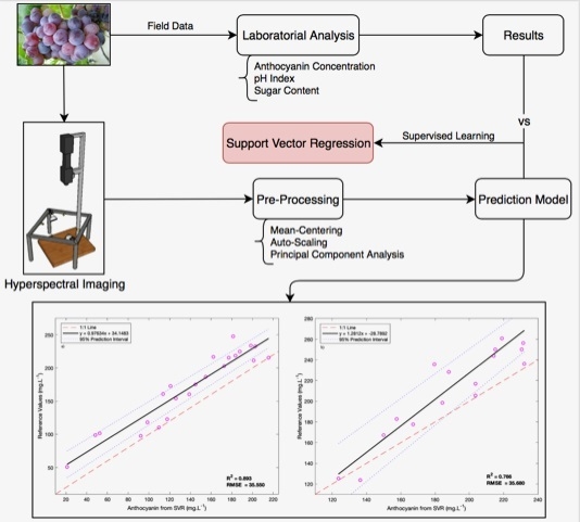
In the present work, we introduce new models combining hyperspectral imaging and support vector regression ([35]) with a Gaussian kernel, implemented with MATLAB software using the parallel computing toolbox with a Compute Unified Device Architecture (CUDA)-enabled NVIDIA Graphics Processing Unit (GPU), to predict oenological parameters in grapes, namely anthocyanin concentration, pH index and sugar content. The study is focused on the generalization ability of the method and on the use of a small number of whole berries per sample, which can be applicable to the selection of the best berries for precision viticulture and for mapping areas in order to improve ripening. The obtained results reveal better performance when compared with previously implemented solutions found in the literature and, unlike the majority of previous works, it includes different varieties and harvest years of wine grape berries. Thus, it is a more detailed study with a capacity for generalization. Section 2 provides a brief description of the varieties of wine grape berries used, an overview of the hyperspectral imaging setup for image-acquisition, details the procedures followed for the reflectance measurements and the techniques applied to build the prediction model, with emphasis on the principal component analysis, support vector regression and cross-validation algorithms, respectively. Section 3 and Section 4 provide a detailed analysis of the results obtained for the different oenological parameters in the study, including a comparison with current state-of-the-art approaches. Section 5 provides general conclusions about the work conducted, alongside future directions for improvement.

2. Materials and Methods

2.1. Grape Sampling

The subject of our study were grapes bunches of the Touriga Franca (TF) variety, considered one of the most important varieties for the production of port wine in the Douro region, due to its resiliency to plant diseases, fruity flavour and intense colour, harvested in the years 2012, 2013 and 2014, from the vineyards of Quinta do Bonfim in Pinhão, Portugal, which is a property of Symington Family Estates, In the year 2015, the samples were collected from the vineyards in Universidade de Trás-os-Montes e Alto Douro, Vila Real, Portugal. In order to achieve the best possible model, it is important to test grapes from the beginning of veraison and maturity, and from areas within the same vineyard under different conditions (sun exposure, water availability, soil quality, among others). A total of 240 samples were collected in the year of 2012 (24 per day), 84 on the year of 2013 (12 per day), 120 in the year of 2014 (12 per day) and 108 in the year of 2015 (12 per day). The samples were collected from three different regions in the vineyard from vine trees with small, medium and large vigour. Laboratory-based, line-scan, hyperspectral image acquisition was performed on fresh grape berries, as described in Section 2.2. Each sample evaluated by hyperspectral imaging was composed of six grape berries randomly collected in a single bunch, removed from bunches with their pedicel still attached. All the samples were then kept frozen, at −18 ºC. The chemical analysis was carried out with the six grape berries being defrosted at room temperature and then crushed in a buffer solution of tartaric acid (pH.3.2) and ethanol (95%) by macerating, and the resulting mixture was kept overnight at 25 °C [36]. The samples were centrifuged (SIGMA centrifuge 3K18, 20 min, 4 °C, spin at 7155 g) and a clear extract was collected and mixed with acidified ethanol (0.1% Hydrochloric Acid). The total anthocyanin concentration was determined photometrically by the SO₂ bleaching method [37]. A Ultraviolet-Visible Spectroscopy (UV/VIS) spectrophotometer (Shimadzu) and 1 cm path length disposable cells were used for spectral measurements at 520 nm and the pigment content, expressed in mg·L⁻¹, was calculated from a calibration curve of malvidin-glucoside. All determinations were performed in duplicate and the juice released was analysed for pH and brix contents according to validated standard methods [38].

In order to test the generalization capacity of the model, 84 and 60 samples (12 per day) were collected in the year 2013 for the Tinta Barroca (TB) and Touriga Nacional (TN) varieties, which are also important varieties for the production of port wine in the Douro region. The sample collection, number of berries per sample, hyperspectral image acquisition and chemical analyses were performed as mentioned previously.

2.2. Experimental Setup for Hyperspectral Imaging

We chose the reflectance mode over the transmittance mode for hyperspectral imaging since, for the same illumination scenario, the intensity of light reflected from the grape is stronger, which facilitates measurements.

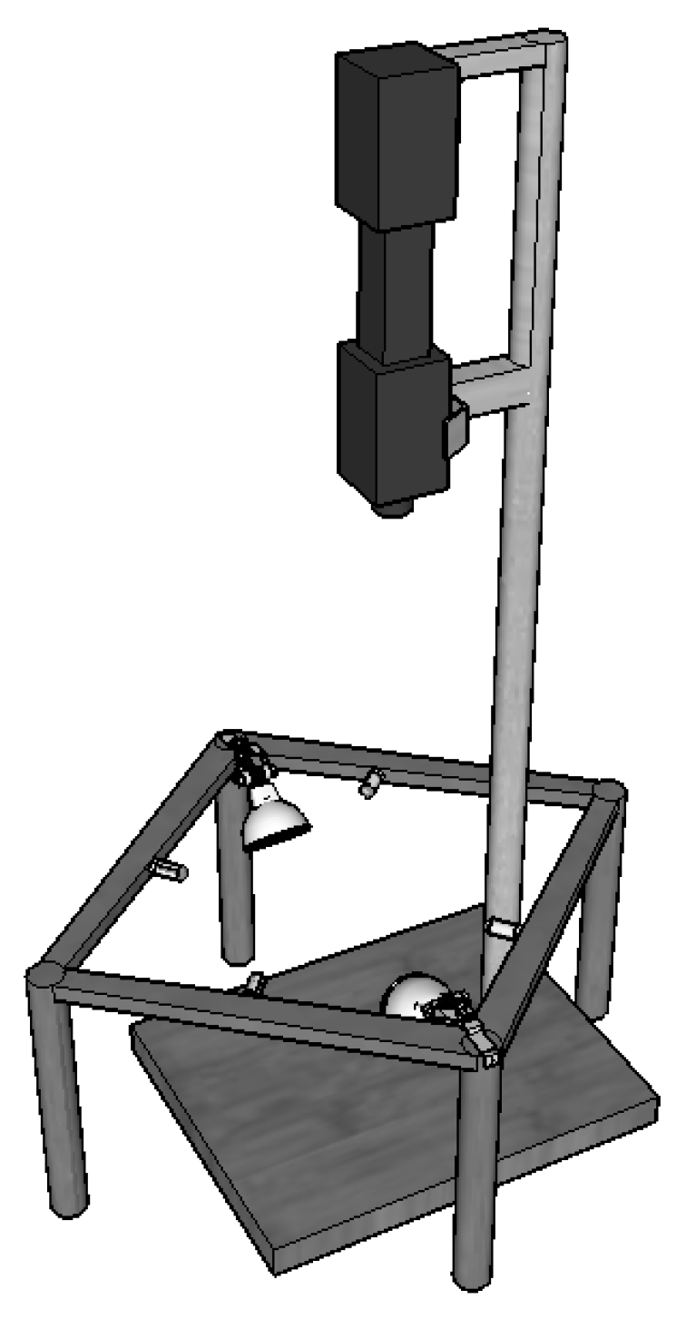
The experimental setup assembled for the images collected used a hyperspectral camera, composed of a JAI Pulnix (JAI, Yokohama, Japan) black and white camera and a Specim Imspector V10E spectrograph (Specim, Oulu, Finland); lighting, using a lamp holder with 300 × 300 × 175 mms (length × width × height) that held four 20 W, 12 V halogen lamps and two 40 W, 220 V blue reflector lamps (Spotline, Philips, Eindhoven, The Netherlands). Both types of lamps were powered by continuous current power supplies to avoid light flickering and the reflector lamps were powered at only 110 V to reduce lighting and prevent camera saturation. The resulting hyperspectral images correspond to a single line over the sample and had 1040 wavelengths (ranging between 380 to 1028 nm, with approximately 0.6 nm width in each channel) × 1392 pixels. The 1392 pixels stand for the spatial dimension over the samples with approximately 110 mm of width. The distance between the camera and the sample base was 420 mm, and the camera was controlled with Coyote software from JAI inside a dark room, at room temperature. Figure 1 illustrates the experimental setup assembled for the hyperspectral image acquisition. After the image acquisition, it is possible to identify the grape berries using image segmentation methods.

Figure 2 shows a hyperspectral image taken by the aforementioned setup, for samples of the TF 2012 variety.

Observing Figure 2, it is possible to see patterns of light absorption, specifically in three main regions, these are where three wine grape berries were placed simultaneously for imaging. A threshold-based segmentation method was then applied to each hyperspectral image to obtain an individual image for each wine grape berry, thus leading to the reflectance measurement step.

2.3. Reflectance Measurements

Reflectance is the quotient between the intensity of the light reflected by an object and the light that illuminates that object, being a function of the wavelength of the light. We chose reflectance as input because the patterns of reflectance and absorption across wavelengths can uniquely identify chemical compounds and because, in contrast to the transmittance and interactance mode, it is possible to perform the imaging without requiring contact between the spectrometer/camera and the sample. For some positions $x$, and at wavelengths $\lambda$, the reflectance $R$ can be expressed as:

$$R\left(x,\lambda \right)=\frac{GI\left(x,\lambda \right)-DI\left(x,\lambda \right)}{SI\left(x,\lambda \right)-DI\left(x,\lambda \right)}$$

(1)

where $GI$ is the intensity of light reflected from the grape; $SI$ is the intensity of light reflected from the Spectralon (which is a total reflectance target); and $DI$ is the dark current signal, which is electronic noise. The dark current signal is measured with the hyperspectral camera lens covered and must be subtracted from the grape and the Spectralon signal because it is independent of the object being imaged and would otherwise distort the calculated reflectance values.

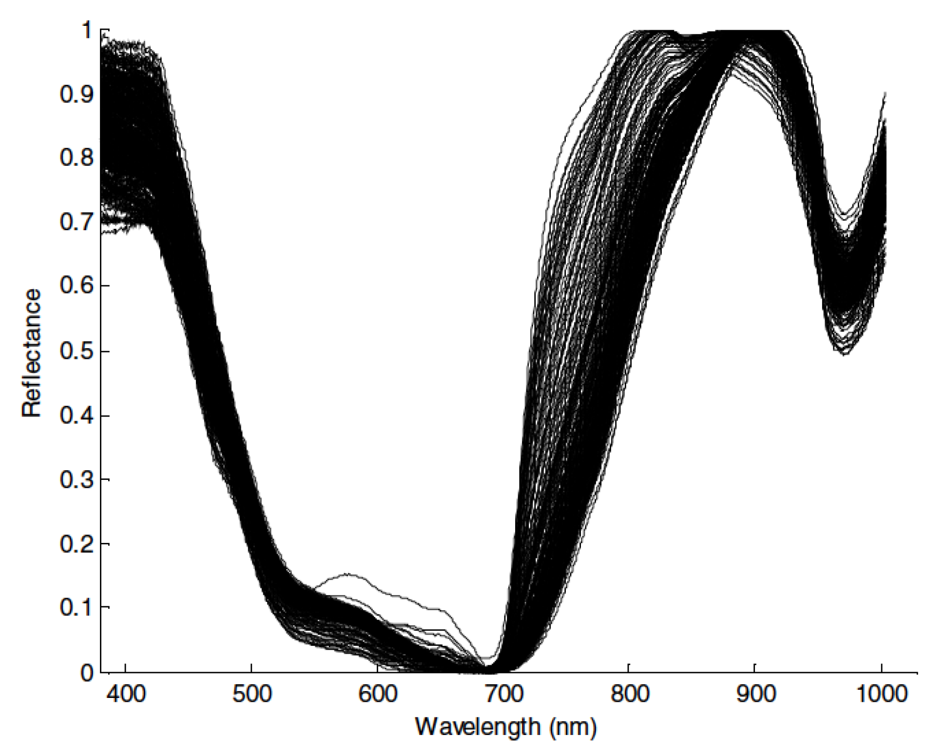
To achieve noise reduction, an accumulation of 32 hyperspectral images on each grape berry were derived for $GI\left(x,\lambda \right)$, $DI\left(x,\lambda \right)$ and $SI\left(x,\lambda \right)$ records. All reflectance measurements for the six grape berries were carried out along the berry “equator”, and for three different berry rotations. In order to create a single reflectance spectrum, all grape point reflectance values were averaged over the spatial dimension and rotations. The resulting spectrum was then normalized (by subtracting the minimum values from each spectrum and dividing by the difference between the maximum and minimum values), in order to eliminate fluctuations in the measured light intensities due to the grape berry size and curvature. Figure 3 presents an example of the reflectance measurements, in the case for the samples of the TF 2012 variety.

2.4. Principal Component Analysis

Due to data complexity, with the dimensionality of the resulting matrix equal to the number of spectral channels measured by the hyperspectral camera (namely 1040), there are difficulties in processing such a large, multivariate dataset. In order to obtain the maximum performance of the machine learning algorithm employed, one must significantly reduce the size of its inputs with some kind of data compression method. Consequently, a principal component analysis (PCA) was performed on the data matrix, extracting the dominant patterns present in the spectra in terms of a complementary set of scores and loadings plots, providing the means to significantly reduce the size of a dataset without losing variability in the data. The PCA was implemented by eigenvalue decomposition of the data covariance matrix and applied to each dataset composed of a different variety and vintage of wine grape berries, together with the mean-centering and auto-scaling methods to normalize the spectra, which subtracts the mean from the original dataset and then divides by its standard deviation. Figure 4 shows the loadings plot for the six first Principal Components (PC) extracted from the TF 2012 variety data matrix.

Observing Figure 4 it is noticeable that there are a large number of peaks throughout the spectrum, with emphasis between 400–700 nm, that are usually related to chemical compounds such as chlorophyll, carotenoids and anthocyanin, while the peeks between 700–800 nm are commonly associated with sugars [38].

A basic assumption in the use of the PCA is that the score and loading vectors corresponding to the largest eigenvalues contain the most useful information relating to the specific problem, and that the remaining ones mainly comprise noise [39]. In general cases, the number of principal components used is chosen by the number of factors with eigenvalues over one, resulting in a percentage of variance explained (that is, the variability accounted for in the data) in a cumulative sum usually between 95–99%. However, in this case the aforementioned assumption might not be true due to the highly complex chemical interactions present in the samples that have an impact on the reflectance measurements. There is no clear answer as to how many factors should be retained for analysis (only general rules of thumb, such as a scree plot analysis) and, since we are using the PCA as a pre-processing step for a supervised learning task, in this paper we decided to treat the number of PCs as another parameter to be optimized during the cross-validation task, in which we used different try-outs to choose the ideal number of PCs. Thus, every model was tested using between one and 50 principal components, saving the best result. We chose 50 PCs as the upper-limit since the results never improved above that number of PCs and the computational cost starts to increase with a higher number of PCs retained for analysis.

2.5. Support Vector Regression

The advantages of using a support vector machine methodology are (both for classification or regression): it has a regularization parameter, making it easier to avoid overfitting; it maps the input vectors to a high-dimensional feature space, so that it is possible to build expert knowledge about a problem via engineering the kernel function; and, most importantly, the algorithm is defined as a convex optimization problem, for which there is no local minima (unlike neural networks or partial least squares regression), using a subset of training points in the decision function, called support vectors, making the computation cost significantly smaller. In order to introduce our choice of the type of regression and kernel employed in the support vector regression framework, below we provide a brief description of the Support Vector (SV) algorithm. A complete mathematical formulation can be found in [40,41].

Given a set of training data $\left\{\left(x_1,y_1\right), \dots , \left(x_n,y_n\right)\right\}\subset \chi \in ℝ$, where $\chi$ denotes the space of the input patterns, the objective is to find a function $f\left(x\right)=\langle w,x\rangle +b, w\in \chi , b\in ℝ$ that has a maximum deviation $\epsilon$ from the real measured targets $y_i$ for all the training data and, simultaneously, is as flat as possible (that is, to be as close to a straight line as possible).

In the case of a linear function, we can express the convex optimization problem as the minimization of the Euclidean norm; however, we must also guarantee that infeasible constraints are dealt with by introducing slack variables ${\xi }_i, {\xi }_i^{*}$, reaching the formulation stated in [35]:

$$\begin{array}{c}\mathrm{minimize:} \frac{1}{2}{\Vert \omega \Vert }^2+C{\displaystyle \sum }_{i=1}^n\left({\xi }_i+{\xi }_i^{*}\right)\\ \mathrm{subject\; to:} \{\begin{array}{c}{y}_i-\left(\omega , x_i\right)-b\le \epsilon +{\xi }_i\\ \left(\omega ,x_i\right)+b-y_i\le \epsilon +{\xi }_i^{*}\\ {\xi }_i,{\xi }_i^{*}\ge 0\end{array}\end{array}$$

(2)

where the constant $C>0$ determines the trade off between the flatness of $f$ and the amount up to which deviations larger than $\epsilon$ are tolerated. An alternative to Vapnik’s ε-SV regression was introduced by [42], named $\nu$-SV regression, where $\epsilon$ is not defined a priori but is itself a variable, where its value is traded off against model complexity and slack variables by means of a constant $\nu \in \left[0,1\right]$.

In order to extend the SV machine to nonlinear functions, one must start by writing the optimization problem in its dual formulation via a Lagrange function from both the objective function and the corresponding constraints by introducing a dual set of variables. Satisfying all the constraints and optimizing the equation, we reach the so-called SV expansion, stated below:

$$f\left(x\right)={\displaystyle \sum }_{i=1}^n\left({\alpha }_i-{\alpha }_i^{*}\right)\left(x_i, x\right)+b$$

(3)

where $\omega$ is completely described as a linear combination of the training patterns, and examples with ${\alpha }_i>0$ are the support vectors.

The chemical processes we are modelling are nonlinear, so the final step is to adapt the SV algorithm to deal with such processes. A computationally cheap way is to map the input vectors into a high-dimensional feature space through some nonlinear mapping, and then to solve the optimization problem in that feature space. With the use of a suitable, nonlinear function $\kappa$ (called kernel), we obtain the nonlinear regression functions of the form:

$$f\left(x\right)={\displaystyle \sum }_{i=1}^n\left({\alpha }_i^{*}-{\alpha }_i\right)·\kappa \left(x_i,x\right)+b$$

(4)

Two major types of kernel can be defined: local kernels (based on distance), which state that only the data that are near each other have an influence on the kernel values; and global kernels (based on the dot product), which state that samples that are far away from each other still have an influence on the kernel value [43].

In the present work, a model with Vapnik’s $\epsilon$-SV algorithm and a Gaussian radial basis local kernel ($\kappa \left(x,x_i\right)=\exp \left(-\gamma \Vert x-x_i\Vert {}^2\right)$) was chosen because it has obtained the least root mean square error for all the models tested (linear, sigmoid, polynomial and Gaussian kernels with Vapnik’s ε–SV regression and Chalimourda’s υ–SV regression, as seen in

Table 2. Experimental results to build the support vector regression model with different loss functions.

			Test Set
			R2	RMSE	PC 1
Anthocyanin Concentration	TF 2012	Vapnik’s $\epsilon$-SV	0.970	11.748 mg·L−1	16
		Chalimourda’s υ–SV	0.943	17.153 mg·L−1	17
pH Index	TF 2012	Vapnik’s $\epsilon$-SV	0.887	0.142	15
		Chalimourda’s υ–SV	0.869	0.144	12
Sugar Content	TF 2012	Vapnik’s $\epsilon$-SV	0.964	0.804 °Brix	15
		Chalimourda’s υ–SV	0.944	0.969 °Brix	16

¹ Principal components used.

and

Table 3. Experimental results to build the support vector regression model with different kernel functions.

			Test Set
			R2	RMSE	PC 1
Anthocyanin Concentration	TF 2012	Gaussian Radial Basis	0.970	11.748 mg·L−1	16
		Linear	0.943	16.749 mg·L−1	18
		Sigmoid	0.943	18.100 mg·L−1	6
		Polynomial	0.932	15.721 mg·L−1	14
pH Index	TF 2012	Gaussian Radial Basis	0.887	0.142	15
		Linear	0.820	0.164	10
		Sigmoid	0.872	0.116	8
		Polynomial	0.867	0.132	19
Sugar Content	TF 2012	Gaussian Radial Basis	0.964	0.804 °Brix	15
		Linear	0.937	1.176 °Brix	8
		Sigmoid	0.910	1.131 °Brix	19
		Polynomial	0.927	1.371 °Brix	20

¹ Principal components used.

). The interval of values for the parameter $C$ of the algorithm and the parameter $\gamma$ in the kernel (the hyper parameters) was determined via a genetic algorithm, resulting in $C\in \left[80;120\right]$ and $\gamma \in \left[0.00001;0.001\right]$, and a random search algorithm was implemented to search these intervals for the first combination of these values lower than an error threshold (mean squared error lower than 0.1) with $\epsilon =0.001$ in the cross-validation procedure, with 10 attempts performed in each different configuration to ensure unbiased predictions.

2.6. N-Fold Cross-Validation with Test Set

To avoid overfitting, a cross-validation approach was employed in the model presented, allowing for the separation of the observations into a training set (to estimate the calibration) and a validation set (to validate the calibration and to correct parameters). In more advanced experiments on the model’s capacity, an independent external test set was used (to evaluate the model performance on an independent set of samples). For further testing the model’s generalization capacity, some of the independent test sets will be composed of new samples of different varieties of wine grape berries not yet seen by the model on the training and validation sets. The cross-validation approach chosen was the n-fold cross-validation method, where the data is split into $n$ folds: $n-1$, used for training, and one for validation, namely the procedure repeated for every fold with a different validation set at each time. The advantage of this kind of approach is that it guarantees that each sample in the dataset is used by the model at least once, contrary to methods that draw data randomly with replacement. The final validation results presented are the average of the results for all the validation sets in each experiment. The training, validation and independent test sets are chosen at random for each run, and the fine-tuning of the model’s hyper parameters only occurs in the cross-validation stage to guarantee an unbiased model.

In order to proceed to a comparison between the present results and state-of-the-art publications, both the root mean square error of the cross-validation and test sets were used (RMSE), alongside the squared correlation coefficient (R²)—these values are defined as follows:

$$RMSE=\sqrt{\frac{{{\displaystyle \sum }}_{i=1}^N{\left({\widehat{y}}_i-y_i\right)}^2}{N-1}}$$

(5)

$$R^2={\left(\frac{{\sigma }_{y\widehat{y}}}{{\sigma }_y{\sigma }_{\widehat{y}}}\right)}^2$$

(6)

where $y_i$ is the reference value, ${\widehat{y}}_i$ is the model estimate, ${\sigma }_{y\widehat{y}}$ is the covariance between $y$ and $\widehat{y}$ and ${\sigma }_y$, ${\sigma }_{\widehat{y}}$ are the respective standard deviations.

Each wine grape variety data had its own training and validation sets (Section 3.1), except for the 2015 vintage that was only used in more advanced experiments. The finetuning of the model’s hyperparameters occurred for all varieties. An independent external test set was used in the study of the TF 2012 variety and in the study of a mixture of samples from different vintages of the TF variety (Section 3.2), since these are the only cases that, in our opinion, presented a sufficient number of samples to use a test set and obtain significant results. To further test the model’s generalization capacity, an independent external test set composed of different varieties of wine grapes was also studied for evaluation of the model’s performance with previously unused varieties in the test set (Section 3.3).

Table 4. Outline of the different experiments performed in the sections below.

	Anthocyanin Concentration		pH Index		Sugar Content
Sections	Train./Val. Set	Test Set	Train./Val. Set	Test Set	Train./Val. Set	Test Set
3.1	TF 2012	2	TF 2012	2	TF 2012	2
	TF 2013	2	TF 2013	2	TF 2013	2
	1	2	TF 2014	2	TF 2014	2
3.2	TF 2012	TF 2012	TF 2012	TF 2012	TF 2012	TF 2012
	TF 2012/13	TF 2012/13	TF 2012/13	TF 2012/13	TF 2012/13	TF 2012/13
	1	1	TF 2012/13/14	TF 2012/13/14	TF 2012/13/14	TF 2012/13/14
	TF 2012/13/15	TF 2012/13/15	TF 2012/13/14/15	TF 2012/13/14/15	TF 2012/13/14/15	TF 2012/13/14/15
3.3	TF 2012/13/15	TB 2013	TF 2012/13/14/15	TB 2013	TF 2012/13/14/15	TB 2013
	TF 2012/13/15	TN 2013	TF 2012/13/14/15	TN 2013	TF 2012/13/14/15	TN 2013

¹ No samples available. ² Not used.

provides detailed information about the experiences conducted and described in each section.

A descriptive statistical analysis was performed to study the datasets used (see Appendix A, Appendix B and Appendix C). ANOVA (one-way analysis of variance) tests were also employed to verify any significant differences between the means of the different sets (see Appendix D, Appendix E and Appendix F), and it was found that there are significant differences in the means between the datasets used for this work.

3. Results

3.1. Model Training and Validation

The validation set results obtained by the models (one for each vintage) for the prediction of the anthocyanin concentration, pH index and sugar content in the different vintages are presented in

Table 5. Results obtained in the validation set for the determination of the anthocyanin concentration, pH index and sugar content of the wine grape berries.

		Validation Set
		R2	RMSE	PC 1	Samples	Samples Mean Value
Anthocyanin Concentration	TF 2012	0.887	19.133 mg·L−1	13	240	160.28 mg·L−1
	TF 2013	0.869	20.053 mg·L−1	7	82	207.18 mg·L−1
pH Index	TF 2012	0.765	0.168	18	240	3.552
	TF 2013	0.673	0.207	9	81	3.718
	TF 2014	0.757	0.130	10	120	3.493
Sugar Content	TF 2012	0.896	1.085 °Brix	20	240	16.925 °Brix
	TF 2013	0.890	1.183 °Brix	7	82	19.446 °Brix
	TF 2014	0.864	1.344 °Brix	13	120	13.552 °Brix

¹ Principal components used.

. For the 2014 vintage of the TF variety there are no laboratory results available for the anthocyanin concentration, preventing the development of a model for that particular vintage.

For each dataset the training and validation were conducted with 10-fold cross-validation for the TF 2012 samples, and with five-fold cross-validation for the remaining vintages (because these have a lower number of samples and reducing the number of folds helps avoiding overfitting in these scenarios).

3.2. Model Behaviour Using Test Sets

The study of the model’s behavior using test sets was performed with the TF 2012, TF 2013, TF 2014 and TF 2015 datasets (except for the prediction of the anthocyanin concentration, where the 2014 vintage results were not available), with 10% of the samples used as an independent test set: the first, with the 2012 vintage (test set: 30 samples); the second, composed of 2012 and 2013 vintages samples (test set: 36 samples); the third, with samples from the 2012, 2013 and 2014 vintages (test set: 50 samples for sugar content and pH index); the fourth, composed of 2012, 2013, 2014 and 2015 vintages (63 samples for sugar content and pH index, 48 samples for anthocyanin concentration).

For each data set the training and validation were conducted with the remaining samples, with 10-fold cross-validation and with the fine-tuning of the hyper parameters in the Support Vector Regression (SVR) models occurring only for the training and validation sets.

Table 6. Results obtained in the external test set for the determination of the anthocyanin concentration, pH index and sugar content of the wine grape berries.

		Test Set			Best State-of-the-Art Result
		R2	RMSE	PC 1	R2	RMSE
Anthocyanin Concentration	TF 2012	0.970	11.748 mg·L−1	16	0.950 2	14.000 mg·L−1	[10]
	TF 2012/13	0.946	17.290 mg·L−1	20
	TF 2012/13/15	0.937	18.019 mg·L−1	38
pH Index	TF 2012	0.887	0.142	15	0.807 2	0.050 2	[19]
	TF 2012/13	0.830	0.170	18
	TF 2012/13/14	0.832	0.144	38
	TF 2012/13/14/15	0.773	0.191	47
Sugar Content	TF 2012	0.964	0.804 °Brix	15	0.959 2	1.026 °Brix 2	[13]
	TF 2012/13	0.948	1.048 °Brix	20
	TF 2012/13/14	0.923	1.411 °Brix	45
	TF 2012/13/14/15	0.934	1.136 °Brix	45

¹ Principal components used. ² Same variety and vintage of wine grape berries used in the training and test sets.

shows the results obtained for the prediction of the anthocyanin concentration, pH index and sugar content on the external test sets while referencing the best result found in the literature for the same experiment, for a direct comparison. For more information regarding these test sets, see Appendix G, Appendix H and Appendix I.

The overall results for the different test sets and for all the oenological parameters under study represent an improvement in the R² and RMSE values in comparison to the ones obtained in the validation sets. Since this is somewhat unusual in machine learning problems,

Table 7. Results obtained by the SVR model in 10 different experiments for the validation and test sets of samples from the TF 2012 vintage for sugar content prediction.

		TF 2012 – Validation Set		TF 2012 – Test Set
		R2	RMSE (°Brix)	R2	RMSE (°Brix)	PC 1
Sugar Content	Exp. 0	0.888	1.095	0.934	1.118	21
	Exp. 1	0.891	1.095	0.933	0.967	21
	Exp. 2	0.888	1.081	0.951	0.931	42
	Exp. 3	0.891	1.103	0.945	0.865	43
	Exp. 4	0.891	1.083	0.942	1.156	28
	Exp. 5	0.885	1.104	0.946	0.908	22
	Exp. 6	0.873	1.199	0.943	0.778	16
	Exp. 7	0.895	1.075	0.947	0.971	44
	Exp. 8	0.887	1.107	0.958	0.827	37
	Exp. 9	0.865	1.232	0.964	0.804	15

¹ Principal components used.

shows a set of experiments that were employed to rule out a possible inherent bias of the SVR algorithm to perform well on the randomly chosen data for the external test sets (that is, a natural predisposition of the algorithm to obtain better results for a certain set of samples).

For each experiment, the samples were independent and chosen at random, which guarantees that the model’s response is unbiased. A total of 10% of the samples were left out to comprise the independent test set, while the remaining samples were used to train and calibrate the model using 10-fold cross-validation.

A possible explanation for the difference in performance in the independent testing phase is that through the pipeline of our model there are various steps where the concern with overfitting [44,45,46] is present. The application of methods to counter this effect, and the sum of all these applications, might then lead the model away from overfitting and lead it into an underfitting situation. This is not a traditional underfitting scenario, where the model cannot capture the relationships in the data during the training stage, but a scenario where the inductive bias of the algorithm is predisposed to lead to increased generalization capacity. Another possibility is that because the optimization method for the hyper-parameters in the SVM tries to optimize the results for the respective test sets on the many different random cross-validation runs, it sacrifices training performance for enhanced generalization capacity [47]. Either way further study on this topic should be conducted.

The enhanced generalization capacity of the model is noticeable by the differences in the results between the validation and test sets present in Table 7: a model with strong inductive biases is likely to benefit when these biases are well suited to the data, which seems to be the case for this work.

3.3. Model Generalization: Different Varieties and Vintages

The last test aimed to further analyse the model’s generalization capacity and involved the use of a mixture of samples from different vintages and varieties of wine grape berries; this is a very important configuration, because if the prediction algorithm cannot handle the variations in the grapes’ oenological parameters that are known to occur between years and varieties, the application of the models becomes more complex since it will require a new model to be used for every different year or for every different variety.

The test of the model’s generalization capacity was performed with two datasets: the first using the samples from all the vintages of the TF variety employed in the training and validation phases, with 10-fold cross validation, and 25% of the samples of the TB variety (23 samples) comprising the independent test set; the second also using all the vintages of the TF variety used in the training and validation stages using 10-fold cross-validation, alongside 25% of the samples of the TN variety (17 samples) used for the external test set.

Figure 5 shows the results obtained for the determination of the anthocyanin concentration in both cases. The number of principal components used were 47 and three, respectively, for each of the datasets. For additional information regarding the samples used, please check Appendix J.

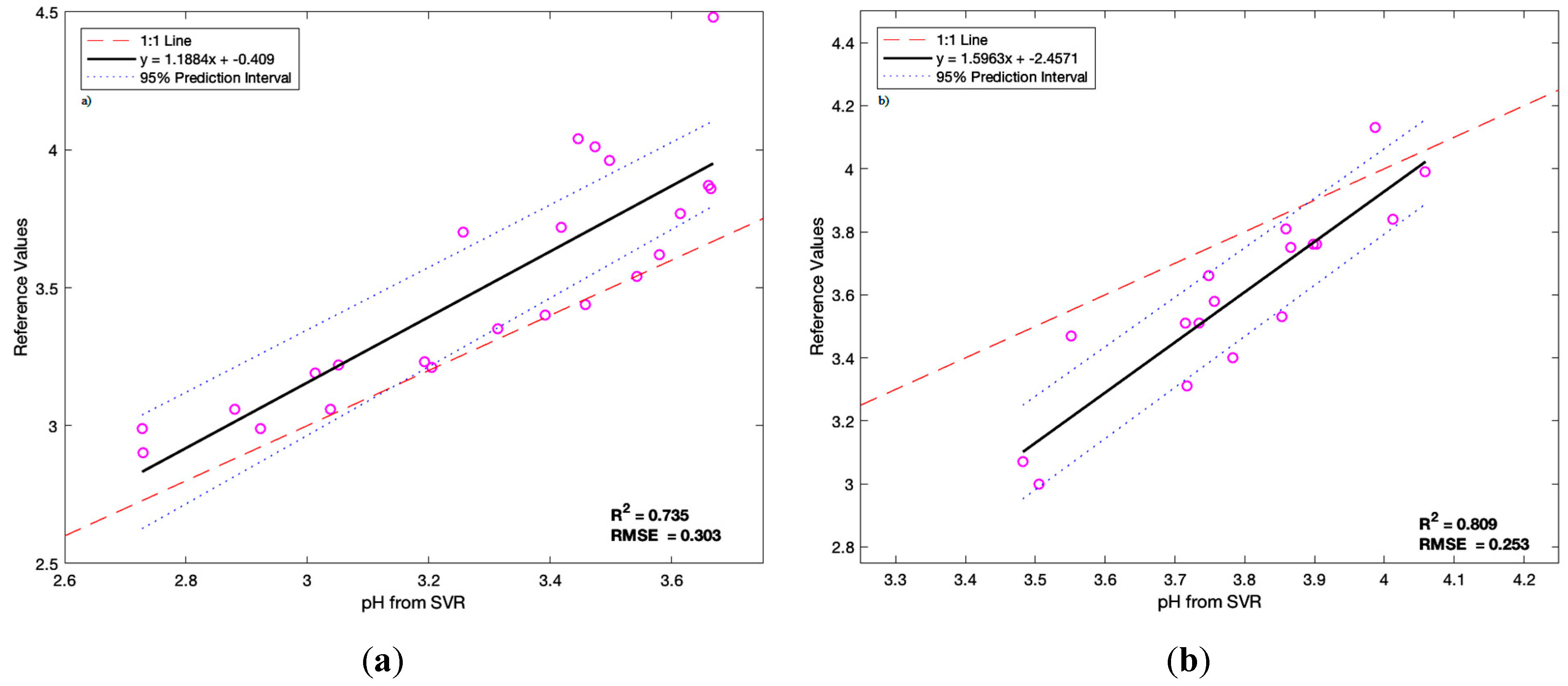
Figure 6 illustrates the outcome for the prediction of the pH index in both cases. The number of principal components used were 11 and 50, respectively, for each of the experiments. More information on the samples used can be seen in Appendix K.

Figure 7 presents the results for the estimation of the sugar content in both cases. The number of principal components used were 45 and 17, respectively, for each of the datasets. Further information regarding the samples is presented in Appendix L.

4. Discussion

4.1. Model Training and Validation

When studying the anthocyanin concentration results (Table 5), 10 folds were used for cross-validation of the Touriga Franca 2012 (with 240 samples), while for the Touriga Franca 2013 (with 82 samples) only five folds were used by the algorithm, so that the model would not skew its learning in the training step. Since the sample set size was smaller, a slight difference between results is considered acceptable; the model was able to obtain similar results and with a smaller number of principal components used, indicating that there is less variance between samples in the 2013 vintage. Overall, the model showed accurate predictions with a small error rate and a good value for the squared correlation coefficient, in line with similar works from the literature. A descriptive statistical analysis of the datasets was conducted (see Appendix A) to study the behaviour of both set of samples.

Analysing the pH index results (Table 5), it is observable that the model underperforms when predicting the pH index in comparison to the determination of anthocyanin concentration (an issue that was also reported in other state-of-the-art approaches, as seen in Table 1). A possible explanation is that since for each run random samples were chosen to compose the validation set, the greatest variation in the pH patterns was reflected in the model’s training step, which had difficulty capturing such relationships in the data with a small number of samples. Also, there is an additional challenge in measuring the pH of wine grape berries, since the acidity is sensitive to small changes in the condition of the sample. The one-way ANOVA analysis showed that there are significant differences in the means (ρ < 0.001) between the TF 2013 and all of the remaining vintages (Appendix E), which might have caused the slight downgrade in the model’s performance. Since the prediction intervals were significantly small and the standard deviations between the samples were close to zero, this may be the reason for the model’s difficulty to learn from these datasets (see Appendix B). A higher number of samples might be required in order to capture the relationships in the data.

Studying the sugar content results (Table 5), it can be seen that the model’s results for all the vintages are accurate, with high squared correlation coefficient values and low root mean square error values. These results indicate that despite the variations in the patterns present in each set, the model was able to capture most of the relations in the data early in the training step. Descriptive statistics for all the sets of samples (see Appendix C) are presented. Regarding the TF 2013 and TF 2014 vintages, it is possible to observe that the latter obtained inferior results, although it had a higher number of samples. Performance of a one-way ANOVA to study meaningful differences in the means for each set of samples revealed that there was a significant difference in the means (ρ < 0.001) between the vintages in the analysis (Appendix F), which might cause the small variations in the results and highlights the model’s capacity to learn from populations of wine grape berries with meaningful statistical differences.

The validation set results presented strongly suggest that the framework is robust, being able to learn the patterns present in the data, but also indicates a need for an increase on the number of samples for the most complex data sets.

4.2. Model Behaviour Using Test Sets

Investigating the anthocyanin concentration results (Table 6) and comparing these with authors with similar methodologies, Chen et al. [17] and Fadock et al. [19] previously used a SVR approach to measure the total anthocyanin concentration of wine grape berries, obtaining an R² of 0.941 and 0.690, respectively, (the error rate was calculated with different measurements and a comparison is not suitable). Looking at the results obtained in the present work, it is noticeable that our approach using an SVR model provided better results, even when a mixture of vintages was used. Previously, Reference [10] had obtained the highest coefficients for the estimation of anthocyanin concentration in external test sets, with a R² of 0.950 and RMSE of 14.000 mg·L⁻¹ using a neural network approach. It is possible to observe that for the TF 2012 data set, our results showed an equivalent but slightly better R² (0.970) and a better RMSE (11.748 mg·L⁻¹). As for the test sets composed of a mixture of TF samples, the results suggest a robust model with a capacity to learn from wine grapes of different vintages. It is also observable that the number of principal components used increased with the variability of the data used and that this increase may be crucial to the model’s adaptability to the differences in the variance of the datasets allowing for more stable predictions.

Analysing the pH index results using test sets (Table 6), while looking for authors using a similar model to predict the pH index of wine grape berries, Reference [9] previously used an approach with least squares support vector machines tuned via a genetic algorithm to measure this chemical compound, obtaining a R² of 0.957 with a RMSE of 0.126 for the validation set. Unfortunately, the results for an external test set were not provided in the published work. The authors in [19] used a SVR model to measure the pH index as well, obtaining a R² of 0.560 and RMSE of 0.050 for a test set composed of samples from different vintages, and a R² of 0.807 and RMSE of 0.050 for a test set composed of samples from the same variety and vintage. Our results showed better performance for predictions on an external test set using a SVR model, with and without different vintages of wine grape berries used in those sets. Despite showing superior results than those obtained by [19] (0.807 for R² and 0.050 for the RMSE) for an external test set, the model’s performance for the pH index was the worst of all the oenological parameters studied, suggesting that a higher number of samples might be required to better incorporate all the data variability into the model.

Studying the sugar content results using test sets (Table 6), for sugar content determination, Reference [9] previously used an approach with least squares support vector machines tuned via a genetic algorithm to measure this chemical compound, obtaining a R² of 0.820 with a RMSE of 0.960 ºBrix for the validation set. The results for an external test set were not provided in the published work. The authors in [19] also used a SVR model to measure sugar content, obtaining a R² of 0.710 and RMSE of 0.870 °Brix for a test set composed of samples from different vintages, and a R² of 0.910 and RMSE of 0.650 °Brix for a test set composed of samples from the same variety and vintage. Our results denote better performance for predictions on an external test set using a SVR model, with and without different vintages of wine grape berries used in those sets. The best previous results for sugar content prediction were from [12], with values of 0.959 and 1.026 °Brix for R² and RMSE, respectively. Our model outperforms the mentioned work for the single vintage dataset (R² of 0.964 and RMSE of 0.804), and presents slightly worse results in the mixture of samples from different vintages.

4.3. Model Generalization: Different Varieties and Vintages

Regarding the model’s generalization capacity for the different vintages and varieties of wine grape berries used in the independent external test sets (Figure 5, Figure 6, Figure 7), despite a slight drop in the model’s performance and a higher error rate in the predictions (which is considered a reasonable outcome due to the fact that these varieties are not found in the training steps, increasing the uncertainty), these results are good indicators with respect to the model’s generalization ability, since they indicate it might not be necessary to build models that require a yearly update of samples, or new samples for each variety. Using a mixture of samples from different vintages and varieties in the test phase is, according to the authors’ knowledge, a rare configuration in general and very unique for samples with a small number of whole berries. Comparing the results with the only work found in the literature using different varieties of wine grapes in the testing phase, we found that [14] obtained a R² of 0.751 and a RMSE of 23.200 mg·L⁻¹ for the determination of anthocyanin concentration, and a R² of 0.710 and a RMSE of 0.176 for the prediction of pH index; our model outperforms the mentioned work for all the datasets studied.

Analysing the values obtained for each oenological parameter, it is clear that the model performs quite well on the determination of the sugar content and anthocyanin concentration, with a minor decrease in the squared correlation coefficient and the root mean squared error. With respect to the determination of the pH index, it is possible that the observed differences between varieties might result from the more complex patterns of pH related to their genetic proximity or distance and the analysis should have this focus for future work. Also, it is reasonable to infer that more samples are needed in order to capture the more complex patterns in the spectra. The difference between the number of principal components retained for analysis in each case should also be highlighted. Although this goes beyond the scope of this paper and should be the subject of future research, we believe that this might happen due to the genetic proximity of the wine grape berries varieties in question; the TN variety is more similar to the TF variety than to the TB variety, which might explain why fewer principal components were required for the TN test set for sugar content and anthocyanin concentration.

5. Conclusions

A hyperspectral imaging technique was combined with a machine learning algorithm (support vector regression) to compose a framework capable of estimating oenological parameters with different varieties and vintages of wine grape berries. The present paper presents a fast, inexpensive and non-destructive type of analysis that provides an alternative to traditional methods when studying wine grape berries during ripening.

The results obtained are competitive in comparison to current state-of-the-art publications in the prediction of sugar content, anthocyanin concentration and pH index, maintaining high performance across different varieties and vintages of wine grapes. This represents a step forward in terms of the study of the generalization capacity, which is very important in order to achieve a model capable of predicting values for a wide variety of wine grapes without the need to capture more and more samples throughout the years to tune the predictor. Moreover, the hyperspectral imaging was conducted in the reflectance mode and with a small number of whole berries, which is a setup rarely found in literature and is relevant when mapping areas in order to improve ripening, selecting the best berries inside each bunch for the production of high quality wines.

Further work should include the study of different pre-processing, dimensionality reduction and feature selection methods, which may represent an improvement in the models’ capacity to capture different patterns in the spectra, especially for the estimation of the pH index, which obtained slightly inferior results. Also, datasets composed of different varieties for the training and test phases should be investigated to promote the development of the generalization capacity while investigating the models’ behaviour when tested without supplementary training.

References

1. Gowen, A.; O’Donnell, C.; Cullen, P.; Downey, G.; Frias, J. Hyperspectral imaging—An emerging process analytical tool for food quality and safety control. Trends Food Sci. Technol. 2007, 18, 590–598. [Google Scholar] [CrossRef]
2. Hall, A.; Lamb, D.W.; Holzapfel, B.; Louis, J. Optical remote sensing applications in viticulture—A review. Aust. J. Grape Wine Res. 2002, 8, 36–47. [Google Scholar] [CrossRef]
3. Fernández-Novales, J.; López, M.-I.; Sánchez, M.-T.; García-Mesa, J.-A.; González-Caballero, V. Assessment of quality parameters in grapes during ripening using a miniature fiber-optic near-infrared spectrometer. Int. J. Food Sci. Nutr. 2009, 60, 265–277. [Google Scholar] [CrossRef] [PubMed]
4. Geraudie, V.; Roger, J.M.; Ojeda, H. Développement d’un appareil permettant de prédire la maturité du raisin par spectroscopie proche infra-rouge. (PIR). Rev. Française d’Oenologie 2010, 240, 2–8. [Google Scholar]
5. Geraudie, V.; Roger, J.M.; Ferrandis, J.L.; Gialis, J.M.; Barbe, P.; Maurel, V.B.; Pellenc, R. A revolutionary device for predicting grape maturity based on NIR spectrometry. Proceedings of (FRUTIC 09) 8th Fruit Nut and Vegetable Production Engineering Symposium, Concepción, Chile, 5–9 January 2009. [Google Scholar]
6. Herrera, J.; Guesalaga, A.; Agosin, E. Shortwave near infrared spectroscopy for non-destructive determination of maturity of wine grapes. Meas. Sci. Technol. 2003, 14, 689–697. [Google Scholar] [CrossRef]
7. Larraín, M.; Guesalaga, A.R.; Agosin, E. A multipurpose portable instrument for determining ripeness in wine grapes using NIR spectroscopy. IEEE Trans. Instrum. Meas. 2008, 57, 294–302. [Google Scholar] [CrossRef]
8. Arana, I.; Jarén, C.; Arazuri, S. Maturity, variety and origin determination in white grapes (Vitis vinifera L.) using near infrared reflectance technology. J. Near Infrared Spectrosc. 2005, 13, 349–357. [Google Scholar] [CrossRef]
9. Cao, F.; Wu, D.; He, Y. Soluble solids content and pH prediction and varieties discrimination of grapes based on visible–near infrared spectroscopy. Comput. Electron. Agric. 2010, 71, S15–S18. [Google Scholar] [CrossRef]
10. Fernandes, A.M.; Franco, C.; Mendes-Ferreira, A.; Mendes-Faia, A.; da Costa, P.L.; Melo-Pinto, P. Brix, pH and anthocyanin content determination in whole Port wine grape berries by hyperspectral imaging and neural networks. Comput. Electron. Agric. 2015, 115, 88–96. [Google Scholar] [CrossRef]
11. Fernandes, A.M.; Oliveira, P.; Moura, J.P.; Oliveira, A.A.; Falco, V.; Correia, M.J.; Melo-Pinto, P. Determination of anthocyanin concentration in whole grape skins using hyperspectral imaging and adaptive boosting neural networks. J. Food Eng. 2011, 105, 216–226. [Google Scholar] [CrossRef]
12. Gomes, V.M.; Fernandes, A.M.; Faia, A.; Melo-Pinto, P. Comparison of different approaches for the Prediction of Sugar Content in Whole Port Wine Grape Berries using Hyperspectral Imaging. Proceedings of ENBIS 14: 14th Annual Conference of the European Network for Business and Industrial Statistics, Linz, Austria, 21–25 September 2014. [Google Scholar]
13. Gomes, V.M.; Fernandes, A.M.; Faia, A.; Melo-Pinto, P. Determination of sugar content in whole Port Wine grape berries combining hyperspectral imaging with neural networks methodologies. Proceedings of 2014 IEEE Symposium on Computational Intelligence for Engineering Solutions (CIES), Orlando, FL, USA, 9–12 December 2014. [Google Scholar]
14. Gomes, V.M.; Fernandes, A.M.; Martins-Lopes, P.; Pereira, L.; Faia, A.; Melo-Pinto, P. Characterization of neural network generalization in the in the determination of pH and anthocyanin content of wine grape in new vintages and varieties. Food Chem. 2017, 218, 40–46. [Google Scholar] [CrossRef] [PubMed]
15. Gomes, V.M.; Fernandes, A.M.; Melo-Pinto, P. Comparison of different approaches for the prediction of sugar content in new vintages of whole Port wine grape berries. Comput. Electron. Agric. 2017, 140, 244–254. [Google Scholar] [CrossRef]
16. Wu, G.-F.; Huang, L.-X.; He, Y. Research on the sugar content measurement of grape and berries by using Vis/NIR spectroscopy technique. Spectrosc. Spectr. Anal. 2008, 28, 2090–2093. [Google Scholar]
17. Chen, S.; Zhang, F.; Ning, J.; Liu, X.; Zhang, Z.; Yang, S. Predicting the anthocyanin content of wine grapes by NIR hyperspectral imaging. Food Chem. 2015, 172, 788–793. [Google Scholar] [CrossRef] [PubMed]
18. Cozzolino, D.; Cynkar, W.; Janik, L.; Dambergs, B.; Francis, I.L.; Gishen, M. Measurement of colour, total soluble solids and pH in whole red grapes using visible and near infrared spectroscopy. Proceedings of 12th Australian Wine Industry Technical Conference, Melbourne, Australia, 24–29 July 2004; pp. 24–29. [Google Scholar]
19. Fadock, M.; Brown, R.B.; Reynolds, A.G. Visible-Near Infrared Reflectance Spectroscopy for Nondestructive Analysis of Red Wine Grapes. Am. J. Enol. Vitic. 2016, 67. [Google Scholar] [CrossRef]
20. Ferrer-Gallego, R.; Hernández-Hierro, J.M.; Rivas-Gonzalo, J.C.; Escribano-Bailón, M.T. Determination of phenolic compounds of grape skins during ripening by NIR spectroscopy. LWT-Food Sci. Technol. 2011, 44, 847–853. [Google Scholar] [CrossRef]
21. González-Caballero, V.; Pérez-Marín, D.; López, M.I.; Sánchez, M.T. Optimization of NIR spectral data management for quality control of grape bunches during on-vine ripening. Sensors 2011, 11, 6109–6124. [Google Scholar] [CrossRef] [PubMed]
22. Hernández-Hierro, J.M.; Nogales-Bueno, J.; Rodríguez-Pulido, F.J.; Heredia, F.J. Feasibility study on the use of near-infrared hyperspectral imaging for the screening of anthocyanins in intact grapes during ripening. J. Agric. Food Chem. 2013, 61, 9804–9809. [Google Scholar] [CrossRef] [PubMed]
23. Janik, L.J.; Cozzolino, D.; Dambergs, R.; Cynkar, W.; Gishen, M. The prediction of total anthocyanin concentration in red-grape homogenates using visible-near-infrared spectroscopy and artificial neural networks. Anal. Chim. Acta 2007, 594, 107–118. [Google Scholar] [CrossRef] [PubMed]
24. Le Moigne, M.; Dufour, E.; Bertrand, D.; Maury, C.; Seraphin, D.; Jourjon, F. Front face fluorescence spectroscopy and visible spectroscopy coupled with chemometrics have the potential to characterise ripening of Cabernet Franc grapes. Anal. Chim. Acta 2008, 621, 8–18. [Google Scholar] [CrossRef] [PubMed] [Green Version]
25. Nogales-Bueno, J.; Hernández-Hierro, J.M.; Rodríguez-Pulido, F.J.; Heredia, F.J. Determination of technological maturity of grapes and total phenolic compounds of grape skins in red and white cultivars during ripening by near infrared hyperspectral image: A preliminary approach. Food Chem. 2014, 152, 586–591. [Google Scholar] [CrossRef] [PubMed]
26. Pal, M.; Mather, P.M. Assessment of the effectiveness of support vector machines for hyperspectral data. Futur. Gener. Comput. Syst. 2004, 20, 1215–1225. [Google Scholar] [CrossRef]
27. Melgani, F.; Bruzzone, L. Classification of hyperspectral remote sensing images with support vector machines. IEEE Trans. Geosci. Remote Sens. 2004, 42, 1778–1790. [Google Scholar] [CrossRef]
28. Mercier, G.; Lennon, M. Support vector machines for hyperspectral image classification with spectral-based kernels. Proceedings of 2003 IEEE International Geoscience and Remote Sensing Symposium (IGARSS ’03), Toulouse, France, 21–25 July 2003; Volume 1, pp. 288–290. [Google Scholar]
29. Rumpf, T.; Mahlein, A.-K.; Steiner, U.; Oerke, E.-C.; Dehne, H.-W.; Plümer, L. Early detection and classification of plant diseases with Support Vector Machines based on hyperspectral reflectance. Comput. Electron. Agric. 2010, 74, 91–99. [Google Scholar] [CrossRef]
30. Cozzolino, D.; Dambergs, R.G.; Janik, L.; Cynkar, W.U.; Gishen, M. Analysis of grapes and wine by near infrared spectroscopy. J. Near Infrared Spectrosc. 2006, 14, 279–289. [Google Scholar] [CrossRef]
31. Noguerol-Pato, R.; González-Barreiro, C.; Cancho-Grande, B.; Martínez, M.C.; Santiago, J.L.; Simal-Gándara, J. Floral, spicy and herbaceous active odorants in Gran Negro grapes from shoulders and tips into the cluster, and comparison with Brancellao and Mouratón varieties. Food Chem. 2012, 135, 2771–2782. [Google Scholar] [CrossRef] [PubMed]
32. Noguerol-Pato, R.; González-Barreiro, C.; Cancho-Grande, B.; Santiago, J.L.; Martínez, M.C.; Simal-Gándara, J. Aroma potential of Brancellao grapes from different cluster positions. Food Chem. 2012, 132, 112–124. [Google Scholar] [CrossRef] [PubMed]
33. Noguerol-Pato, R.; González-Barreiro, C.; Simal-Gándara, J.; Martínez, M.C.; Santiago, J.L.; Cancho-Grande, B. Active odorants in Mouratón grapes from shoulders and tips into the bunch. Food Chem. 2012, 133, 1362–1372. [Google Scholar] [CrossRef]
34. Tarter, M.E.; Keuter, S.E. Effect of rachis position on size and maturity of Cabernet Sauvignon berries. Am. J. Enol. Vitic. 2005, 56, 86–89. [Google Scholar]
35. Vapnik, V.N. The Nature of Statistical Learning Theory; Springer: New York, NY, USA, 1995; Volume 8. [Google Scholar]
36. Carbonneau, A.; Champagnol, F. Nouveaux systemes de culture integre du vignoble. Programme AIR-3-CT 93; Unpublished Protocol. 1993. [Google Scholar]
37. Ribéreau-Gayon, P.; Stonestreet, E. Determination of anthocyanins in red wine. Bull. la Société Chim. Fr. 1965, 9, 2649–2652. [Google Scholar]
38. Organisation Internationale de la Vigne et du Vin. Recueil des Méthodes Internationales D’analyse des vins et des Moûts; O.I.V.: Paris, France, 1990. [Google Scholar]
39. Wold, S.; Esbensen, K.; Geladi, P. Principal Component Analysis. Chemom. Intell. Lab. Syst. 1987, 2, 37–52. [Google Scholar] [CrossRef]
40. Basak, D.; Pal, S.; Patranabis, D.C. Support Vector Regression. Neural Inf. Process. Lett. Rev. 2007, 11, 203–224. [Google Scholar]
41. Smola, A.J.; Schölkopf, B. A Tutorial on Support Vector Regression. Stat. Comput. 2004, 14, 199–222. [Google Scholar] [CrossRef]
42. Chalimourda, A.; Schölkopf, B.; Smola, A.J. Experimentally optimal ν in support vector regression for different noise models and parameter settings. Neural Netw. 2004, 17, 127–141. [Google Scholar] [CrossRef]
43. Smits, G.F.; Jordaan, E.M. Improved SVM regression using mixtures of kernels. In Proceedings of the 2002 International Joint Conference on Neural Networks (IJCNN’02) (Cat. No.02CH37290), Honolulu, HI, USA, 12–17 May 2002; Volume 3, pp. 2785–2790. [Google Scholar]
44. Bengio, Y.; Grandvalet, Y. No Unbiased Estimator of the Variance of K-Fold Cross-Validation. J. Mach. Learn. Res. 2004, 5, 1089–1105. [Google Scholar]
45. Kohavi, R. A study of cross-validation and bootstrap for accuracy estimation and model selection. In Proceedings of the 1995 International Joint Conference on Artificial Intelligence, IJCAI, Montreal, QC, Canada, 20–25 August 1995; Volume 14, pp. 1137–1145. [Google Scholar]
46. Cawley, G.C.; Talbot, N.L.C. Preventing Over-Fitting during Model Selection via Bayesian Regularisation of the Hyper-Parameters. J. Mach. Learn. Res. 2007, 8, 841–861. [Google Scholar]
47. Schutten, M.; Wiering, M. An Analysis on Better Testing than Training Performances on the Iris Dataset. Proceedings of Belgian Dutch Artificial Intelligence Conference, Amsterdam, The Netherlands, 10–11 November 2016. [Google Scholar]
Figure 1. Experimental setup used for hyperspectral imaging.
Remotesensing 10 00312 g001
Figure 2. Hyperspectral image of samples of the TF 2012 variety before segmentation and reflectance measurements.
Remotesensing 10 00312 g002
Figure 3. Reflectance measurements for the TF 2012 variety samples.
Remotesensing 10 00312 g003
Figure 4. Loadings plot for the TF 2012 variety data matrix.
Remotesensing 10 00312 g004
Figure 5. Results for the determination of the anthocyanin concentration in the external test sets to further study the generalization capacity; (a) TB 2013 samples; (b) TN 2013 samples.
Remotesensing 10 00312 g005
Figure 6. Results for the prediction of the pH index in the external test sets to further study the generalization capacity; (a) TB 2013 samples; (b) TN 2013 samples.
Remotesensing 10 00312 g006
Figure 7. Results for the estimation of the sugar content in the external test sets to further study the generalization capacity; (a) TB 2013 samples; (b) TN 2013 samples.
Remotesensing 10 00312 g007