Article

Comparison between AMSR2 Sea Ice Concentration Products and Pseudo-Ship Observations of the Arctic and Antarctic Sea Ice Edge on Cloud-Free Days

1
Chinese Antarctic Center of Surveying and Mapping, Wuhan University, Wuhan 430079, China
2
Key Laboratory of Polar Surveying and Mapping, National Administration of Surveying, Mapping and Geoinformation, Wuhan 430079, China
*
Authors to whom correspondence should be addressed.
Remote Sens. 2018, 10(2), 317; https://doi.org/10.3390/rs10020317
Submission received: 3 January 2018 / Revised: 17 February 2018 / Accepted: 17 February 2018 / Published: 20 February 2018
(This article belongs to the Special Issue Uncertainty in Remote Sensing Image Analysis)

Abstract

:
In recent years, much attention has been paid to the behavior of passive microwave sea ice concentration (SIC) products for marginal ice zones. Based on the definition of ice edges from ship observations, we identified pseudo-ship observations (PSO) and generated PSO ice edges from twelve cloud-free moderate-resolution imaging spectroradiometer (MODIS) images. Two SIC products of the advanced microwave scanning radiometer 2 (AMSR2) were compared at the PSO ice edges: ARTIST (arctic radiation and turbulence interaction study) sea ice (ASI-SIC) and bootstrap (BST-SIC). The mean values of ASI-SIC pixels located at ice edges were 10.5% and 10.3% for the Arctic and the Antarctic, respectively, and are below the commonly applied 15% threshold, whereas the mean values of corresponding BST-SIC pixels were 23.6% and 27.3%, respectively. The mean values of both ASI-SIC and BST-SIC were lower in summer than in winter. The spatial gaps among the 15% ASI-SIC ice edge, the 15% BST-SIC ice edge and the PSO ice edge were mostly within 35 km, whereas the 15% ASI-SIC ice edge matched better with the PSO ice edge. Results also show that the ice edges were located in the thin ice region, with a mean ice thickness of around 5–8 cm. We conclude that the 15% threshold well determines the ice edge from passive microwave SIC in both the Arctic and the Antarctic.

Graphical Abstract

1. Introduction

Sea ice, as a major component of the cryosphere, significantly influences the polar and global climate [1]. The heat and mass transfer and interaction between ocean and atmosphere are insulated and influenced by the sea ice distribution [2,3]. The decreasing sea ice coverage is one of the most obvious indicators of global warming, which can be estimated from the retreat of sea ice edges [4,5].
Satellite passive microwave data, which are weather- and daylight-independent, have been used to identify trends and variability in ice extent in the polar region as well as in locating ice edges [6]. Since the launch of the first satellite radiometer, Nimbus-5 electrically scanning microwave radiometer in 1972, several satellite radiometers have been launched, including the Nimbus-7 scanning multichannel microwave radiometer (SSMR), the first defense meteorological satellite program special sensor microwave/imager (SSM/I), special sensor microwave imager/sounder (SSMIS) and the advanced microwave scanning radiometer Earth observing system (AMSR-E). Satellite launches are accompanied by the development of passive microwave SIC algorithms, such as the NASA-team (NT), the enhanced NASA-team (NT2), BST and ASI. More recently, AMSR2, as a successor of AMSR-E, provides brightness and temperature at a relatively fine resolution. ASI and BST algorithms have been applied on AMSR2 and the daily ASI-SIC and BST-SIC map based on AMSR2 has been accessible since August 2012.
Comparisons have been made between different SIC algorithms. On the one hand, a specific algorithm has been tested on different satellite sensors. Comiso and Parkinson [7] evaluated the SIC, sea ice extent and area derived by BST and NT2 from AMSR-E and SSM/I at the Arctic and the Antarctic. They found that the difference of BST on different sensors was much smaller than the difference of BST and NT2 on one sensor. On the other hand, comparisons have been done among different algorithms. Spreen et al. [8] compared ASI, NT2 and BST on AMSR-E with ship-based observation (OBS) and found correlations equal to 0.80, 0.79, and 0.81, respectively. Heygster et al. [9] compared ASI, NT2 and BST on AMSR-E in the Arctic and Antarctic, and found biases of SIC below 2% and root-mean-square errors between 7% and 11%. Ozsoy-Cicek et al. [10] compared NT2 and BST on AMSR-E with OBS in the Antarctic and found that the SIC derived from NT2 had slightly higher correlation with OBS-SIC than with BST. Beitsch et al. [11] compared AMSR-E ASI, BST and NT2 with OBS and found that ASI-SIC and BST-SIC had an insignificant bias and that BST-SIC had the lowest root mean square deviation (RMSD) (<13%), whereas NT2-SIC had the largest bias among the three algorithms in all seasons. Beitsch et al. [12] found that BST and ASI of AMSR-E are more in accordance with OBS, as compared with BST and ASI applied to SSM/I data. Year-round RMSD values of BST and ASI are 13.2% and 14.3% for SSM/I, and 11.6% and 13.3% for AMSR-E. Ivanova et al. [13] compared thirteen sea ice algorithms, and found ASI performs well over ice, but is sensitive to cloud liquid water over the marginal ice zone (MIZ).
In general, algorithms tend to underestimate the ice concentration in the region of thin ice as well as in the vicinity of the ice edge, especially if the MIZ is diffuse [14,15]. The accuracy of ice concentration in the MIZ attracts the interest of researchers, and in-depth study would be of great value. Ozsoy-Cicek et al. [2] compared the sea ice edge of AMSR-E-based SIC using NT2 and the BST retrieval algorithm with OBS. They found a good correlation inside the ice pack; however, in the MIZ, the correlation decreased. Both NT2 and BST tend to underestimate low ice concentration.
The 15% ice concentration threshold has been used to determine the sea ice extent in climatology analysis. This threshold, however, is not always consistent in different studies. For the Arctic, the threshold has been set between 15% and 30% [16,17]. For the Antarctic, the threshold even reached 40% [18]. As for in-situ validation, the ship observations were recorded using the protocol specified by the Antarctic Sea Ice Processes and Climate (ASPeCt) program [19]. Worby and Comiso [6] evaluated the ice edge location with OBS in the Antarctic and found that PM ice edges were 1–2° of latitude south of the OBS. Heinrichs et.al [20] found that the ice edges determined from AMSR-E data and SAR data were within one AMSR-E grid square (12.5 km). Ozsoy-Cicek et al. [2] compared AMSR-E sea ice edges with NIC (the U.S. National Ice Center) sea ice edges as well as OBS in the Antarctic. Their results indicated that the sea ice edge detected by AMSR-E was further south and that AMSR-E was ineffective in the detection of low SIC.
Because the number of ship observations located at the sea ice edge is limited, Zhao et al. [21] proposed a method to generate PSO from optical satellite images, and used PSO to assess the quality of AMSR-E ASI SIC products at the ice edge in the Antarctic. They found that the mean ASI-SIC at the ice edge was 13%, i.e. close to the 15% threshold, and that the correlations between ASI-SIC and PSO crossing the boundary were low. In this paper, we modified this method and applied it to evaluate AMSR2 ASI and BST SIC at the ice edge in both the Arctic and the Antarctic, as well as to further assess the reliability of a 15% SIC threshold for both poles.

2. Materials and Methods

2.1. Dataset I: AMSR2 ASI and BST SIC Products

AMSR2 was launched with the satellite “Shizuku” (GCOM-W1) on May 18, 2012, and it has sent back data since August 2012. AMSR2 BST-SIC products utilize vertically polarized brightness temperature (Tb) measured by 19 and 37GHz channels and with a resolution of 12.5 km [22]. The AMSR2 ASI-SIC product utilizes information from a higher frequency, 89 GHz, and results in an increased spatial resolution of 6.25 km [8]. However, the high frequency also introduced more sensitivity to the effects of atmospheric cloud liquid water and water vapor as a cost [13,23]. In this study, both AMSR2 ASI-SIC and BST-SIC were downloaded from the Institute of Environmental Physics, University of Bremen, Germany (https://seaice.uni-bremen.de/start/data-archive/).

2.2. Dataset II: MODIS

Of the twelve MODIS/Terra scenes used in this study, six scenes were located in the Arctic and six scenes were located in the Antarctic. The locations of image scenes and acquisition time are shown in Figure 1 and Table 1. MOD09 (MODIS Surface Reflectance) is a seven-band product computed from the MODIS Level 1B bands. It corrects for the effects of atmospheric gases and aerosols. We selected MOD09GA data providing daily surface reflectance at a 500 m resolution (Bands 1–7). The surface reflectance of Band 1 (620–670 nm), Band 3 (459–479 nm) and Band 4 (545–565 nm) was used to identify sea ice from open water and then attain SIC. MOD09GA data were downloaded from the Level-1 and atmosphere archive and distribution system (https://ladsweb.nascom.nasa.gov/). They were geometrically corrected and transformed towards a geographic projection by the MODIS Reprojection Tool.

2.3. Dataset III: SMOS Thin Sea Ice Thickness

An L-band microwave sensor, SMOS (soil moisture and ocean salinity) working at 1.4 GHz, has been used to retrieve the daily thickness of thin sea ice (SIT) since October 2013. Thin ice thickness is derived from an empirical method using the horizontal and vertical polarized brightness temperatures [24]. The spatial resolution of SMOS SIT is 12.5km. We adopted SMOS SIT to check the distribution of thickness of thin ice along the ice edge. The purpose was to compare the performance of 15% ASI-SIC and 15% BST-SIC from the ice thickness perspective. The SMOS data were downloaded from the Institute of Environmental Physics, University of Bremen, Germany (https://seaice.uni-bremen.de/start/data-archive/).

2.4. Data Processing I: MODIS Sea Ice Binary Map and PSO

The MODIS visible bands were used to differentiate open water (OW) from ice based upon a MODIS albedo threshold. Three MODIS bands (B1, B3 and B4) were derived from MOD09GA data and their reflectance (RefB1, RefB3 and RefB4) was combined to obtain the broadband top-of the-atmosphere albedo (Av) as [25]
Av = 0.3265 × RefB1 + 0.4364 × RefB3 + 0.2366 × RefB4
An ice–water threshold was employed to Av to obtain binary sea ice maps. If Av ≥ 0.1, the pixel was labeled as 1 (ice), else as 0 (water) [26]. The binary sea ice maps were resampled to 250 m resolution and re-projected into polar stereographic projection. For this step, we prepared 250 m resolution binary sea ice maps, which were used to generate pseudo-ship points.
According to the ASPeCt, the sea ice edge equals the northernmost occurrence of sea ice of at least 10% SIC as estimated within a circle of 1 km radius from the ship [6]. This rule is used to define PSO. To generate the PSO, we needed to inspect an ice–water map with a 1 km radius from a point at an image, rather than of from a ship. To do so, we applied a moving average filter (9 × 9) to each 250 m resolution pixel on the binary sea ice map (Figure 2), in order to estimate the PSO-SIC within a 1 km radius. The output PSO map was still at 250 m resolution, but the value of a pixel represented the SIC of the surrounding 1 km radius. Next, 10% PSO contours were identified as PSO ice edges [21]. We then traced these ice edges and marked all ASI-SIC and BST-SIC pixels which pass through the PSO ice edges and compared the sample mean to the 15% threshold value.

2.5. Data Processing II: Comparison of Ice Edges

Sea ice edges were derived from ASI-SIC and BST-SIC maps by setting a 15% threshold, called the 15% ASI-SIC ice edge and the 15% BST-SIC ice edge, respectively. They were compared with sea ice edges derived from the pseudo-ship observation to find their performance in the determination of sea ice edges in the MIZ. After that, ice thickness at the edges was extracted from SMOS images to examine their ability to define “edge” from the thickness perspective.

3. Results

From the summary in Table 2, we note that the mean values of ASI-SIC at ice edges are approximate 10%, well below the 15% threshold, in both the Arctic and the Antarctic. In summer, these mean values decrease to 8%. The only case in which ASI-SIC exceeds 15% occurs in the Antarctic winter, whereas the mean values of BST-SIC at the ice edges are well above 15%, most of which are even above 20% except for 11.8% in the Arctic summer. In general, ASI tends to underestimate SIC at ice edge on cloud-free days, whereas BST behaves adversely.
From the perspective of ASI, the mean value and standard deviation of ASI-SIC at PSO ice edges are lower in summer than in winter. In summer, the mean value of ASI-SIC in the Arctic equals 8.8%, close to that in the Antarctic (8.1%). The histogram and box chart indicate that nearly half of ASI-SIC values were close to 0%, and most of the other values are below 20%. In winter, the mean value of ASI-SIC in the Antarctic equals 15.7%, i.e. higher than in the Arctic (11.3%). Nearly half of ASI-SIC values are close to 10%, and most of the other values are below 60%. Furthermore, only the ASI-SIC in the Antarctic winter is not significantly different from the 15% threshold, according to the significant test. We also observe a second peak in the ASI-SIC histogram around 15% in the Antarctic winter.
The mean values of BST-SIC at PSO ice edges are lower in summer than in winter. In summer, the mean value of BST-SIC in the Arctic equals 11.8%, i.e. much lower than that in the Antarctic (26.1%). The histogram and box chart indicate that most BST-SIC values are close to 0% in the Arctic, whereas in the Antarctic most of them are above 10%. In winter, the mean value of BST-SIC in the Arctic equals 28.5%, again lower than in the Antarctic (30.5%). The histogram and box chart indicate that half of BST-SIC values are between 10% and 50%, many appears with large values close to 1, especially in the Antarctic winter. Only the mean value of BST-SIC in Arctic summer is not significantly different from the 15% threshold.
Next, we demonstrated the spatial locations of three kinds of ice edges by means of four examples. From Scene C, taken in the Arctic summer, we observe that the 15% ASI-SIC ice edge and the 15% BST-SIC ice edge are very close to each other, i.e. mainly within one BST pixel (12.5 km) and also very close to the PSO ice edge (Figure 3). Especially for the compact ice edge in region B, the three ice edges highly coincide. Since BST-SIC has a coarser resolution, however, it can cross the ice-water boundary with different SIC values, e.g. 0% on one side and 40% on the other side of the edge. Along diffuse ice edges like in region A, the 15% ASI-SIC and 15% BST-SIC ice edges differ more than 25 km from the PSO ice edges in thin ice regions. Such vague ice boundaries or MIZ are common in the Arctic summer when melting ice can easily be broken by waves and winds. We plotted the corresponding ASI-SCI and BST-SCI at PSO ice edges using histograms (Figure 3) to check their statistical distributions. As expected, many zero values occur and these result into low mean values for both ASI-SIC and BST-SIC (2.1% and 5.1%, respectively).
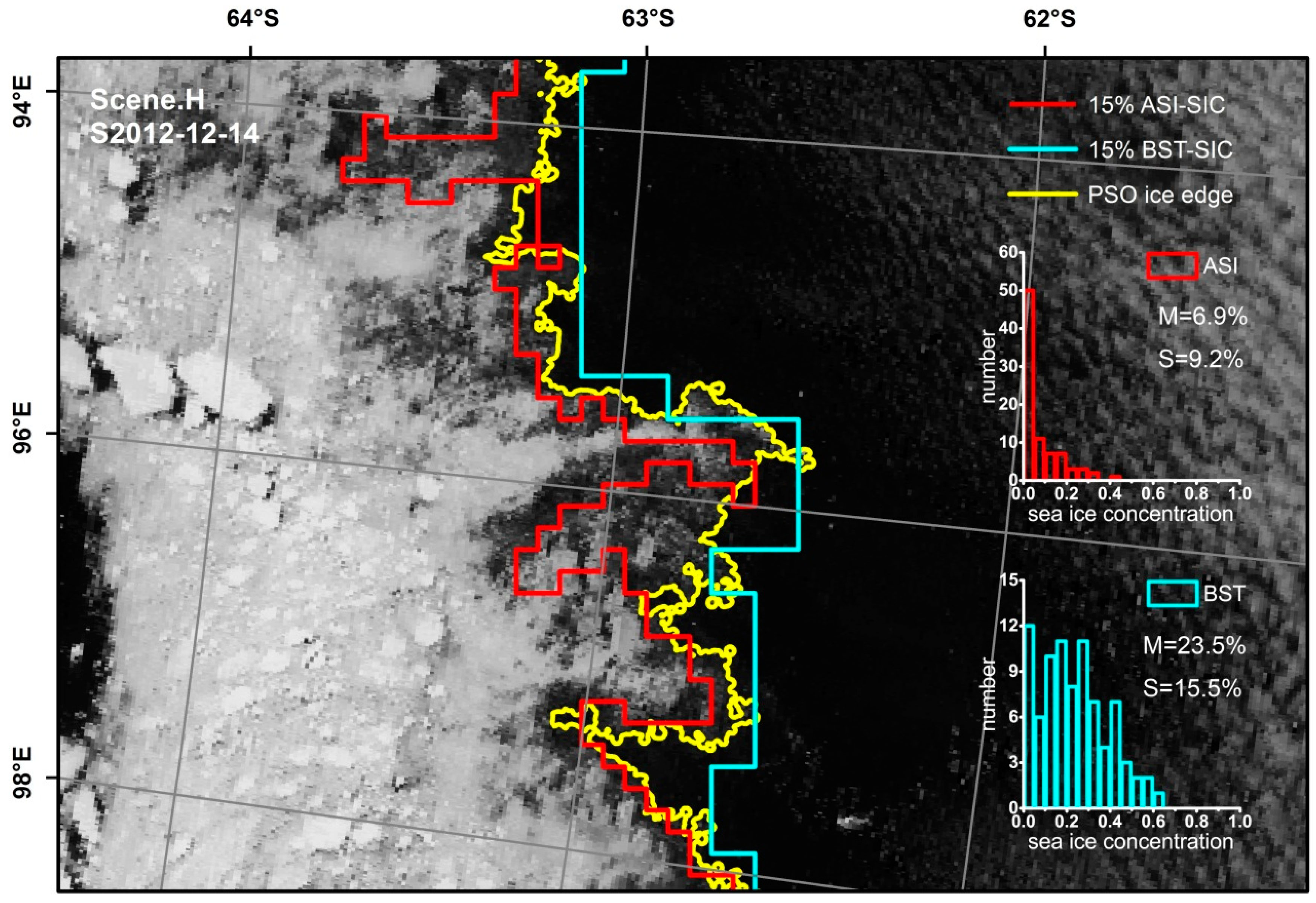
Figure 4 shows the gradually changing ice zone between sea ice and open water in the Antarctic summer. The contour of 15% ASI-SIC is closer to thicker ice and further away from PSO ice edges in sparsely spread ice zones. The mean value of ASI-SCI along the PSO ice edge equals 6.9%, i.e. well below the 15% threshold. In contrast, the 15% BST-SIC contour is closer to the PSO ice edges and the corresponding mean BST-SCI equals 23.5%. We note that the 15% BST-SIC contours enclose all thin ice zones and sometimes even overestimate the extent.
Compared to Figure 3 and Figure 4, the ice edge in 
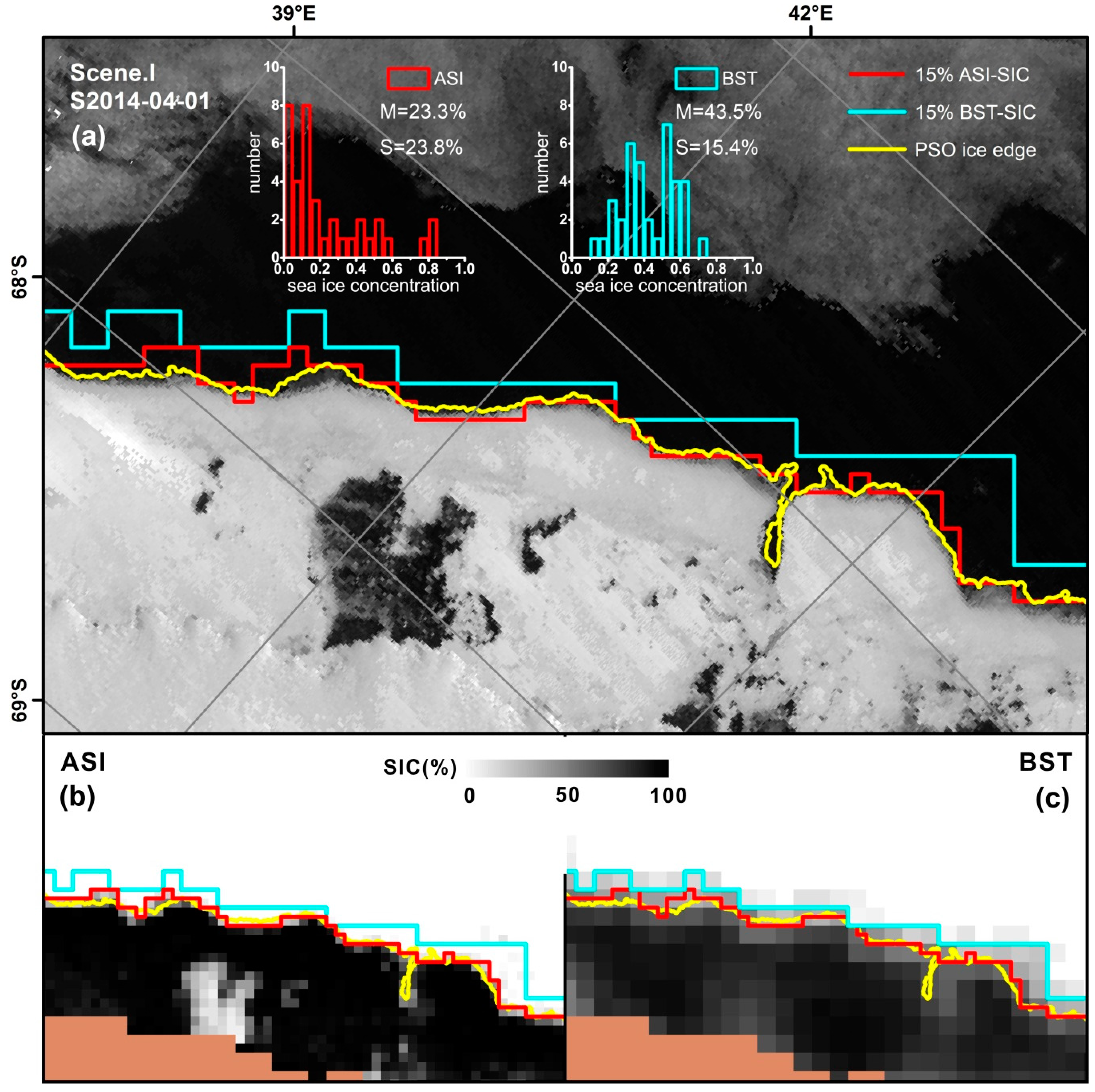
Figure 5 is more compact. This MODIS image was acquired for the Antarctic autumn when sea ice starts to freeze. The 15% ASI-SIC ice edge is close to the PSO ice edge, except for a linear opening which was miscaptured due to the coarse resolution of ASI pixels. The mean value of ASI-SIC crossing PSO ice edges equals 23.3% with a standard deviation of 23.8%, whereas the 15% BST-SIC ice edge is further away from the PSO ice edge than the 15% ASI-SIC. Figure 4b,c illustrate the corresponding daily AMSR2 ASI-SIC product and AMSR2 BST-SIC product, respectively. From these two subfigures, we observe that ASI-SIC has a sharp boundary between ice and non-ice zones, whereas BST-SIC has a vague transition from high SIC to low SIC and then to zero values. Since the 15% BST-SIC ice edge is located mostly outward, the average SIC along this line is high, achieving 43.5% on average.
Figure 6 shows the ice edge in the Arctic in winter time. In region A, the three contours perfectly occur along a single line. In region B, the 15% BST-SIC ice edge is close to the PSO edge; however, the 15% ASI-SIC ice edge is close to thicker ice and further away from the PSO ice edge. Mean values of ASI-SIC and BST-SIC for the whole scene equal 15.2% and 25.6% respectively. Comparing the two histograms in Figure 6, we can observe that the many zero ASI-SIC values decrease its mean value. Some of these come from the diffuse ice edge in region B, where ASI cannot detect newly formed thin ice. We then utilized thin ice thickness retrieved from SMOS to investigate the thickness distribution in this region.
Three histograms were made based on the ice thickness at SMOS pixels along the contours of 15% ASI-SIC, 15% BST-SIC and the PSO ice edge (Figure 7). We found that ice thicknesses crossing all the contours are above zero. Most SMOS pixels at the BST-SIC ice edge have thickness values below 15cm, but the ice thickness at the ASI-SIC ice edge could be above 20cm. The mean ice thickness of the 15% ASI-SIC ice edge, the 15% BST-SIC ice edge and the PSO ice edge are equal to 8.0 cm, 5.3 cm and 6.6 cm, respectively. The ice thickness variation along 15% BST SIC (2.5 cm) is smaller than that along the 15% ASI-SIC ice edge.
To quantify the bias and accuracy of the 15% threshold line against the PSO ice edge, we obtained statistics on the average distance and gap area between the PSO ice edge and the 15% ASI-SIC and the 15% BST-SIC ice edges. Results are listed in Table 3. In general, the average distance from PSO ice edge to the 15% ASI-SIC ice edge are smaller than that to the 15% BST-SIC ice edge. This is consistent with the finer spatial resolution of ASI-SIC than BST-SIC. After transferring the distance unit (km) into the pixel size, we found that both ASI and BST ice edges are within a three-pixel width to the PSO ice edge. The total area is obtained by calculating the area difference among the three edges and summing the total of the entire scene. The gap areas between 15% BST-SIC and PSO edges are larger than those between 15% ASI-SIC and PSO edges: the largest difference equals 5664 km2, which is approximately equal to an area of 36 BST pixels.
According to the mean SIC along the PSO ice edge reported in Table 2, the 10% ASI-SIC and 20% BST-SIC ice edges were chosen as the alternatives to compare with the 15% threshold contours in Scene H (Figure 8). By visual comparison, we observe that the 10% ASI-SIC and 20% BST-SIC match slightly better with the PSO ice edges. This improvement, however, is small, and further study is needed to draw a solid conclusion.

4. Discussion

The objective of this study was to compare ASI-SIC and BST-SIC products at sea ice edges. Previous research [8] examined the performance of different SIC products with OBS data, but rarely focused on MIZ. Zhao et al. [21] proposed a method to automatically identify sea ice edges from high resolution images and applied it to AMSR-E ASI-SIC products. This study tested the more recent sensor AMSR2 and was extended to ASI-SIC and BST-SIC products for both the Arctic and the Antarctic.
The result indicated that the 15% AMSR2 ASI-SIC and BST-SIC and the PSO ice edge derived from MODIS were close in space. In particular, some parts of the 15% ASI-SIC ice edge and the PSO ice edge were within a one-pixel distance (Figure 4). The 15% ASI-SIC ice edges were closer to thick ice and the mean ASI-SIC value at the PSO ice edge was below 15%, as can be observed from Figure 5 and Figure 6 as well as from Table 2. This was consistent with a previous study in which passive microwave products tended to underestimate SIC at the ice edge. The bias can be caused by the following. First, in the melting season, the brash ice at the sea ice edge, saturated by waves and melted snow, may cause ASI algorithms to underestimate SIC [6]. Second, the 89 GHz channel may, in atmospheric cloud liquid water and water vapor, have a negative effect on brightness temperatures. This effect takes place more frequently in summer and early autumn at MIZ [13]. The ASI algorithm uses a weather filter process method to remove spurious ice concentration close to open water [8]. Third, thin ice occurs more commonly along the ice edge and SIC algorithms usually have a low accuracy in those regions.
In contrast, the 15% BST-SIC ice edges were often closer to open water as compared to the PSO ice edge. The mean BST-SIC value at the PSO ice edge was well above 15%. The reasons for overestimating SIC were the following. First, wind may compact the ice in winter time, thus creating a well-defined ice edge. In passive microwave products with coarse resolution, however, the SIC at the ice edge may rise from 0% at one pixel to 100% at its neighboring pixel. Worby and Comiso [6] also found that in the Antarctic ice growth season, the distance from the northernmost occurrence of ice to consolidated ice was usually 18–36 km. This results in both mean values of ASI-SIC and BST-SIC being higher than 20%, such as in Figure 4. Secondly, the resolution of BST-SIC is lower than ASI-SIC, so the 15% BST-SIC ice edge may be further away from the PSO ice edge than that of the 15% ASI-SIC due to the mixed pixel problem.
The mean value of AMSR2 ASI-SIC at the PSO ice edge was 10.3% in the Antarctic, which was close to the mean AMSR-E ASI-SIC value 13% in Zhao et al. [21]. Both were significantly lower than 15%. The difference between AMSR-E and AMSR2 can be overlooked because the basic performance of AMSR2 is similar to AMSR-E based on the data continuity [27]. We also found that in the Antarctic winter the mean value of BST-SIC at the PSO ice edge was 30.5%, which is slightly higher than that of SSMI BST-SIC (19%) in Worby and Comiso [6], though both of them were above 15%.
MODIS data served as validation data in this study. The albedo classified ice and water, and a threshold equal to 0.1 was set in this research. However, the area below this threshold may have a mixture of ice crystals and open water or black nilas [28] that may result in MODIS PSO uncertainty. Additionally, the image of MOD09GA is a snapshot of a single day, whereas the AMSR2 ASI-SIC and BST-SIC are daily average products. This may cause a mismatch of the sea ice edge, especially on windy days when the sea ice edge moves at a high speed.
The mean SMOS SIT along the 15% ASI-SIC ice edge, the 15% BST-SIC ice edge and the PSO ice edge were equal to 8.0 cm, 5.3 cm and 6.6 cm, respectively. According to the World Meteorological Organization (WMO), ice thickness below 10cm is new ice, i.e. recently formed ice [29]. Thus, the ice edge was located at a new ice region. Results indicated that the BST algorithm can recognize the thinnest ice in the new ice rather than open water, whereas ASI tends to recognize thicker ice.

5. Conclusions

This study compared ASI-SIC with BST-SIC at the PSO ice edge extracted from MODIS images. In total, 12 scenes of MODIS from the Arctic and the Antarctic in summer and winter have been processed and analyzed. The results demonstrated that the mean values of ASI-SIC pixels located at the PSO ice edge were 10.5% and 10.3% in the Arctic and the Antarctic, respectively. The mean values of BST-SIC pixels located at the PSO ice edge were equal to 23.6% and 27.3% in the Arctic and the Antarctic, respectively. Both mean values of ASI-SIC and BST-SIC in summer were lower than those in winter. All mean values of ASI-SIC were below 15%, except in the Antarctic winter, whereas all mean values of BST-SIC were above 20% except in the Arctic summer. The 15% ASI-SIC ice edge and the 15% BST-SIC ice edge were close to the PSO ice edge at the compact boundary. In diffuse MIZs, most 15% ASI-SIC ice edges were closer to the thicker ice zone than the 15% BST-SIC ice edge, showing that ASI tends to underestimate SIC. In contrast, BST overestimates SIC and the 15% BST-SIC ice edge is usually closer to the open water than the PSO. The average distance between the 15% BST-SIC ice and the PSO ice edge are larger than that between the 15% ASI-SIC and the PSO ice edge. SMOS ice thickness demonstrated that the 15% ASI-SIC, the 15% BST-SIC and the PSO ice edge were located within new ice regions. Mean ice thicknesses were equal to 8.0 cm, 5.3 cm and 6.6 cm, respectively.
The PSO method was successfully extended to both the Arctic and the Antarctic. It can identify ice edge pixels and edge lines by means of a clear and objective definition. Currently, operational ice services around the world are still using diverse resources to manually identify sea ice edges from multi-source images. This PSO method is promising to further develop automatic ice charting.

Acknowledgments

This work was supported by the National Natural Science Foundation of China (No. 41576188 and 41606215). The authors want to thank the Institute of Environmental Physics (IEP), University of Bremen, Germany, for providing ASI and BST concentration data as well as SMOS data, and the Level-1 and Atmosphere Archive & Distribution System for the MODIS data. We also thank two referees and Prof. Alfred Stein for their valuable comments and editing which improved the manuscript.

Author Contributions

Xiaoping Pang and Xi Zhao generated the idea and drafted the manuscript. Jian Pu carried out the analysis. Meng Qu provided support in programming and data analysis. Zian Cheng and Qing Ji contributed to analysis method and reviewed and edited the manuscript. The final draft of the manuscript was revised and approved by all of the authors.

Conflicts of Interest

The authors declare no conflict of interest.

References

  1. Shokr, M.; Sinha, N. Introduction. In Sea Ice: Physics and Remote Sensing; John Wiley & Sons: Hoboken, NJ, USA, 2015. [Google Scholar]
  2. Ozsoy-Cicek, B.; Xie, H.; Ackley, S.F.; Ye, K. Antarctic summer sea ice concentration and extent: comparison of ODEN 2006 ship observations, satellite passive microwave and NIC sea ice charts. Cryosph. 2008, 3, 1–9. [Google Scholar] [CrossRef]
  3. Aulicino, G.; Fusco, G.; Kern, S.; Budillon, G. Estimation of Sea-Ice Thickness in Ross and Weddell Seas from SSM/I Brightness Temperatures. IEEE Trans. Geosci. Remote Sens. 2014, 52, 4122–4140. [Google Scholar] [CrossRef]
  4. Vihma, T. Effects of Arctic Sea Ice Decline on Weather and Climate: A Review. Surv. Geophy. 2014, 35, 1175–1214. [Google Scholar] [CrossRef]
  5. Comiso, J.C.; Meier, W.N.; Gersten, R. Variability and trends in the Arctic Sea ice cover: Results from different techniques. J. Geoph. Res.-Oceans 2017. [Google Scholar] [CrossRef]
  6. Worby, A.P.; Comiso, J.C. Studies of the Antarctic sea ice edge and ice extent from satellite and ship observations. Remote Sens. Environ. 2004, 92, 98–111. [Google Scholar] [CrossRef]
  7. Comiso, J.C.; Parkinson, C.L. Arctic sea ice parameters from AMSR-E data using two techniques and comparisons with sea ice from SSM/I. J. Geoph. Res.-Oceans 2008. [Google Scholar] [CrossRef]
  8. Spreen, G.; Kaleschke, L.; Heygster, G. Sea ice remote sensing using AMSR-E 89-GHz channels. J. Geoph. Res. Oceans 2008. [Google Scholar] [CrossRef]
  9. Heygster, G.; Wiebe, H.; Spreen, G.; Kaleschke, L. AMSR-E Geolocation and Validation of Sea Ice Concentrations Based on 89GHz Data. J. Remote Sens. Soc. Jp. 2009, 29, 226–235. [Google Scholar]
  10. Ozsoy-Cicek, B.; Ackley, S.F.; Worby, A.; Xie, H.; Lieser, J. Antarctic sea-ice extents and concentrations: comparison of satellite and ship measurements from International Polar Year cruises. Ann. Glaciol. 2015, 52, 318–326. [Google Scholar] [CrossRef]
  11. Beitsch, A.; Kern, S.; Kaleschke, L. Comparison of AMSR-E sea ice concentrations with aspect ship observations around Antarctica. In Proceedings of the Geoscience and Remote Sensing Symposium, Munich, Germany, 22–27 July 2012. [Google Scholar]
  12. Beitsch, A.; Kern, S.; Kaleschke, L. Comparison of SSM/I and AMSR-E Sea Ice Concentrations With ASPeCt Ship Observations Around Antarctica. IEEE Trans. Geosci. Remote Sens. 2014, 53, 1985–1996. [Google Scholar] [CrossRef]
  13. Ivanova, N.; Pedersen, L.T.; Tonboe, R.T.; Kern, S.; Heygster, G.; Lavergne, T.; Sørensen, A.; Saldo, R.; Dybkjær, G.; Brucker, L.; Shokr, M. Satellite passive microwave measurements of sea ice concentration: An optimal algorithm and challenges. Cryosph. Disc. 2015. [Google Scholar] [CrossRef]
  14. Agnew, T.; Howell, S. The use of operational ice charts for evaluating passive microwave ice concentration data. Atmosphere 2003. [Google Scholar] [CrossRef]
  15. Liu, J.; Scott, K.A.; Gawish, A.; Fieguth, P. Automatic Detection of the Ice Edge in SAR Imagery Using Curvelet Transform and Active Contour. Remote Sens. 2016, 8, 480. [Google Scholar] [CrossRef]
  16. Divine, D.V.; Dick, C. Historical variability of sea ice edge position in the Nordic Seas. J. Geoph. Res. Oceans 2006. [Google Scholar] [CrossRef]
  17. Andersen, S.; Tonboe, R.; Kern, S.; Schyberg, H. Improved retrieval of sea ice total concentration from spaceborne passive microwave observations using numerical weather prediction model fields: An intercomparison of nine algorithms. Remote Sens. Environ. 2006. [Google Scholar] [CrossRef]
  18. Fowler, C.; Emery, W.J.; Maslanik, J. Satellite-derived evolution of Arctic sea ice age: October 1978 to March 2003. IEEE Geosci. Remote Sens. Lett. 2004. [Google Scholar] [CrossRef]
  19. Worby, A.P.; Ackley, S.F. Antarctic research yields circumpolar sea ice thickness data. EOS Trans. Am. Geoph. Union 2000. [Google Scholar] [CrossRef]
  20. Heinrichs, J.F.; Cavalieri, D.J.; Markus, T. Assessment of the AMSR-E Sea Ice-Concentration Product at the Ice Edge Using RADARSAT-1 and MODIS Imagery. IEEE Trans.n Geosci. Remote Sens. 2006. [Google Scholar] [CrossRef]
  21. Zhao, X.; Su, H.; Stein, A.; Pang, X. Comparison between AMSR-E ASI sea-ice concentration product, MODIS and pseudo-ship observations of the Antarctic sea-ice edge. Ann. Glaciol. 2015, 56, 45–52. [Google Scholar] [CrossRef]
  22. Comiso, J.C.; CavalierI, D.J.; Parkinson, C.L.; Gloersen, P. Passive microwave algorithms for sea ice concentration: A comparison of two techniques. Remote Sens. Environ. 1997, 60, 357–384. [Google Scholar] [CrossRef]
  23. Oelke, C. Atmospheric signatures in sea-ice concentration estimates from passive microwaves: Modelled and observed. Int. J. Remote Sens. 1997, 18, 1113–1136. [Google Scholar] [CrossRef]
  24. Huntemann, M.; Heygster, G.; Kaleschke, L.; Krumpen, T.; Mäkynen, M.; Drusch, M. Empirical sea ice thickness retrieval during the freeze-up period from SMOS high incident angle observations. Cryosph. Disc. 2014, 7, 4379–4405. [Google Scholar] [CrossRef] [Green Version]
  25. Liang, S.; Shuey, C.J.; Russ, A.L.; Fang, H.; Chen, M.; Walthall, C.L.; Daughtry, C.; Hunt, R., Jr. Narrowband to broadband conversions of land surface albedo: II. Validation. Remote Sens. Environ. 2003, 84, 25–41. [Google Scholar] [CrossRef]
  26. Cavalieri, D.J.; Markus, T.; Hall, D.K.; Ivanoff, A.; Glick, E. Assessment of AMSR-E Antarctic Winter Sea-Ice Concentrations Using Aqua MODIS. IEEE Trans. Geosci. Remote Sens. 2010. [Google Scholar] [CrossRef]
  27. Imaoka, K.; Kachi, M.; Kasahara, M.; Ito, N.; Nakagawa, K.; Oki, T. Instrument performance and calibration of AMSR-E and AMSR2. Int. Arch. Photogramm. Remote Sens. Spat. Inf. Sci 2010, 38, 13–16. [Google Scholar]
  28. Cavalieri, D.J.; Markus, T.; Hall, D.K.; Gasiewski, A.J.; Klein, M.; Ivanoff, A. Assessment of EOS Aqua AMSR-E Arctic Sea Ice Concentrations Using Landsat-7 and Airborne Microwave Imagery. IEEE Trans. Geosci. Remote Sens. 2006, 44, 3057–3069. [Google Scholar] [CrossRef]
  29. WMO (World Meteorological Organization). WMO Sea Ice Nomenclature, Terminology, Codes, and Illustrated Glossary; WMO/OMM/ÂÌÎ No.259; Secretariat World Meteorol. Org.: Geneva, Switzerland, 1970. [Google Scholar]
Figure 1. Location of the twelve moderate-resolution imaging spectrometer (MODIS) scenes in Arctic and Antarctic.
Remotesensing 10 00317 g001
Figure 2. Moving average filter (9 × 9) for an image of 250 m resolution. The hatched center cell represents the ship, the solid line circle with 1 km radius represents the observation range, and the pseudo-ship observation (PSO) sea ice concentration (SIC) is obtained from the grey cells.
Remotesensing 10 00317 g002
Figure 3. The contour of the 15% ASI-SIC, 15% BST-SIC and the PSO ice edge overlaid on the MOD09GA for the Arctic at 7 August 2014.
Remotesensing 10 00317 g003
Figure 4. The contour of the 15% ASI-SIC, 15% BST-SIC and the PSO ice edge overlaid on the MOD09GA, for the Antarctic on 14 December 2014.
Remotesensing 10 00317 g004
Figure 5. Contour of the 15% ASI-SIC, 15% BST-SIC and the PSO ice edge overlaid on (a) MOD09GA, (b) ASI-SIC, (c) BST-SIC, for the Antarctic at 1 April 2014.
Remotesensing 10 00317 g005
Figure 6. Contour of the 15% ASI-SIC, 15% BST-SIC and the PSO ice edge overlaid on the MOD09GA, for the Arctic at 16 February 2014.
Remotesensing 10 00317 g006
Figure 7. Contour of the 15% ASI-SIC, 15% BST-SIC and the PSO ice edge overlaid on the SMOS ice thickness map, on 16 February 2013.
Remotesensing 10 00317 g007
Figure 8. Comparison between contours of the 15% threshold and alternatives with PSO ice edges. (a) 15% ASI-SIC and 10% ASI-SIC, (b) 15% BST-SIC and 20% BST-SIC overlaid on the MOD09GA, at 14 December 2014, Antarctic.
Remotesensing 10 00317 g008
Table 1. Times of the twelve MODIS scenes in the Arctic and Antarctic.
ARCTICANTARCTIC
Scene A2014.07.29Scene G2012.12.21
Scene B2014.08.08Scene H2012.12.14
Scene C2014.08.07Scene I2014.04.01
Scene D2013.03.24Scene J2013.04.08
Scene E2014.03.27Scene K2013.04.11
Scene F2013.02.16Scene L2013.01.01
Table 2. Comparison of advanced microwave scanning radiometer 2 (AMSR2) ARTIST (arctic radiation and turbulence interaction study) sea ice (ASI) and bootstrap (BST) SIC at PSO ice edges. The mean of and BST-SIC samples are tested against the 15% threshold by the z test. The statistical distribution of ASI-SIC and BST-SIC are shown in the histograms (dash line: 15% SIC) and boxplots (solid line: median, dash line: mean).
ArcticAntarctic
ASI-SICBST-SICASI-SICBST-SIC
All dataNo. of pixels 307307332332
Mean (%) 10.523.610.327.3
Std Dev (%) 19.62415.519.4
z test −3.98*6.297*−5.585*11.573*
Histogramnumber Remotesensing 10 00317 i001 Remotesensing 10 00317 i002 Remotesensing 10 00317 i003 Remotesensing 10 00317 i004
Box Chart Remotesensing 10 00317 i005
SummerNo. of pixels 8989237237
Mean(%) 8.811.88.126.1
Std dev(%) 17.217.91319.6
z test −3.404*−1.713−8.19 *8.671*
Histogramnumber Remotesensing 10 00317 i006 Remotesensing 10 00317 i007 Remotesensing 10 00317 i008 Remotesensing 10 00317 i009
Box Chart Remotesensing 10 00317 i010
WinterNo. of pixels 2182189595
Mean(%) 11.328.515.730.5
Std dev(%) 20.524.719.518.6
z test 2.703*8.049*0.3328.136*
Histogramnumber Remotesensing 10 00317 i011 Remotesensing 10 00317 i012 Remotesensing 10 00317 i013 Remotesensing 10 00317 i014
Box Chart Remotesensing 10 00317 i015
* Statistically significant at the 0.05 level.
Table 3. Differences among three ice edges statistics by average distances and total gap areas. Minus means the line of 15% ASI-SIC/BST-SIC is on the outside of the PSO edge.
15% ASI-SIC & PSO edge15% BST-SIC & PSO edge
SceneDateAverage Distance (km)Total gap Area (km2)Average Distance (km)Total Gap Area (km2)
Scene CN2014-08-07–10–625–31–2031
Scene FN2013-02-167723232266
Scene HS2012-12-14171484–8–1250
Scene IS2014-04-01–3–508–11–5664

