Comparison of Three Methods for Estimating GPS Multipath Repeat Time


1
College of Surveying and Geo-informatics, TongJi University, Shanghai 200092, China
2
Key Laboratory of Geographic Information Science, Ministry of Education, East China Normal University, Shanghai 200241, China
3
Engineering Center of SHMEC for Space Information and GNSS, East China Normal University, Shanghai 200241, China
*
Authors to whom correspondence should be addressed.
Remote Sens. 2018, 10(2), 6; https://doi.org/10.3390/rs10020006
Submission received: 19 December 2017
/
Revised: 12 January 2018
/
Accepted: 19 January 2018
/
Published: 23 January 2018
(This article belongs to the Special Issue Multi-Constellation Global Navigation Satellite Systems: Methods and Applications)
Abstract
:Sidereal filtering is an effective method for mitigating multipath error in static GPS positioning. Using accurate estimates of multipath repeat time (MRT) in sidereal filtering can further improve the performance of the filter. There are three commonly used methods for estimating the MRT: Orbit Repeat Time Method (ORTM), Aspect Repeat Time Adjustment (ARTA), and Residual Correlation Method (RCM). This study utilizes advanced sidereal filtering (ASF) adopting the MRT estimates derived by the three methods to mitigate the multipath in observation domain, then evaluates the three methods in term of multipath reduction in both coordinate and observation domain. Normally, the differences between the MRT estimates from the three methods are less than 1.2 s on average. The three methods are basically identical in multipath reduction, with RCM being slightly better than the other two methods, whereas for a satellite affected by orbit maneuver (satellite number 13 in this study), the MRT estimated by the three methods differ by up to tens of seconds, and the RCM- and ARTA-derived MRT estimates are better than ORTM-derived ones for ASF multipath reduction. The RCM shows a slight advantage in multipath mitigation, while ORTM is the one of lowest computation and ARTA is the optimal one for real-time ASF. Thus, the best MRT estimation method for practical applications depends on which criterion overweighs the others.
1. Introduction
For a GPS station, the multipath effects depend on the surroundings of the specific site and the geometric relationship between the GPS receiver (antenna) and satellites [1,2]. Thus, it is still a challenge to develop a general multipath correction model for different GPS stations. As other errors (e.g., troposphere delay, ionosphere delay, and phase center variation) are well modeled, multipath becomes a major error source in GPS positioning. In general, a GPS satellite revisits a specified ground-based GPS site on basis of the sidereal day. Assuming that the surrounding conditions related to this site are constant every day, the multipath effects for this site appear to be repeated at a sidereal day as well. Based on this time-domain repeatability, Bock et al. [3,4] proposed a method named sidereal filtering to mitigate multipath error for static GPS positioning. Sidereal filtering has been well developed and widely applied (e.g., [5,6,7,8,9,10,11,12,13,14,15]). The general principle of sidereal filtering is the construction of a multipath correction model from the residuals of coordinates or observables of the previous day(s), then the correction of the data of the subsequent day(s) by subtracting the corresponding correction value for each epoch.
Wübbena et al. [5] found that the repeat time of GPS satellite was not equal to an exact sidereal day (23 h 56 min 04 s), and there was a bias of several seconds between the repeat time of GPS constellation and a sidereal day. Hence, if a sidereal day is adopted as a multipath repeat time (MRT), the inaccuracy of several seconds will affect the multipath reduction of sidereal filtering. Some studies have demonstrated that using accurate MRT estimates to implement sidereal filtering can further reduce the variance of the coordinate time series (e.g., [6,7]). Filtering with accurate MRT estimates has better performance in mitigating the multipath of the period from 25 to 1000 s [6,7]. Thus, it is necessary to estimate accurate MRTs in order to improve the multipath mitigation of sidereal filtering. Generally, three methods are used to estimate the MRT. Choi et al. [6] adopted GPS broadcast ephemerides to calculate the orbit repeat time of individual satellite. Their results show that the repeat time of GPS satellites is not equal to a sidereal day, and is satellite-dependent. For brevity, their method is referred as the orbit repeat time method (ORTM). Larson et al. [8] and Agnew and Larson [16] used another method that calculates the time interval between GPS satellite arriving the same topocentric position on two consecutive days as MRT estimate. Their method was named aspect repeat time adjustment (ARTA) [8]. Ragheb et al. [9] adopted a third method. They estimated MRT based on the correlation between two residual (coordinate residual or observable residual) time series from two consecutive days. This method is referred as the residual correlation method (RCM).
Since the three methods adopt different mechanisms and algorithms, they have different computational costs and different application requirements, and their calculated MRT values may be different. Previous studies have compared ORTM with ARTA, but did not take the RCM method into consideration for their comparisons [10,16]. In addition, their comparisons excluded the MRT estimates of the GPS satellites that were affected by orbit maneuvering. In general, the estimated MRT values are within a range from 86,145 to 86,165 s (hereinafter referred as normal range). When a satellite is affected by orbit maneuver, its repeat time may deviate from the normal range by tens to hundreds of seconds [6,17], and it is still unknown what the differences between the MRT estimates derived by the three methods for such a satellite. This study compares the MRT estimates derived by the three methods (ORTM, ARTA, and RCM) for both satellites affected and unaffected by orbit maneuver, and assesses the three methods in aspects of multipath reduction, robustness, computational cost, and real-time application. The MRT estimates from the three methods are adopted in advanced sidereal filtering (ASF), respectively, to mitigate the multipath error of GPS observables. Then, we compare the performances of the three methods in multipath reduction after ASF corrections. The ASF is a modified sidereal filtering, which corrects the multipath of observables for each satellite with its MRT estimate [11,13].
2. Methods
2.1. Orbit Repeat Time Method (ORTM)
For a GPS satellite, according to Kepler’s third law, the square of the orbital period is directly proportional to the cube of the semi-major axis of its orbit. The orbit period in inertial space is given by
where is the semi-major axis of the orbit and is the standard gravitational parameter of the Earth. Equation (1) can also be written as
where is the mean motion of the satellite. In the reference frame on the rotating earth, the repeat time of a satellite relative to a ground-based GPS station is two times its orbit period. Adding a correction to mean motion , the repeat time of the satellite is given by
In the right side of Equation (3), and are constants, the value of semi-major axis and mean motion correction can be acquired from the broadcast ephemerides (broadcast ephemerides provide the value of ). is the repeat time of the satellite and is considered to be an estimate of MRT for this satellite.
The time interval of orbit data in GPS broadcast ephemeris is two hours. Thus, a full-day broadcast ephemeris contains 12 or 13 epochs’ data for each satellite. Reading in a GPS broadcast ephemeris, our ORTM program calculates the repeat time of individual satellite at each epoch. For a single day, the program computes the mean and the standard deviation (STD) of the repeat time values of all 12 or 13 epochs for each satellite. The mean for a satellite is the MRT estimate of that satellite on that day. The STD for a satellite is a criterion for evaluating the stability of repeat time estimates of that satellite for the same day.
2.2. Aspect Repeat Time Adjustment (ARTA)
For a GPS satellite and a ground-based GPS site, we denote the unit vector of line-of-sight of the receiver-to-satellite at epoch as . Assuming that day 1 and day 2 are two consecutive days, and day 2 is after day 1, denotes the angle between and , is the unit vector at epoch on day 1, is the unit vector at epoch on day 2. The can be calculated by
For a given , is a function with the argument . If gives a minimal value when , then
is the repeat time of this satellite and is an estimate of MRT for the satellite.
The unit vectors can be calculated when the a priori coordinate of the ground-based GPS site and the coordinate of satellites are known. Since the IGS precise ephemeris directly provides the coordinates of satellites, we adopt this type of ephemeris in implementing ARTA for simplifying the calculation. Normally, a daily IGS precise ephemeris provides the satellite coordinates of 96 epochs (interval of 15 min). For each GPS satellite, our ARTA program calculates the unit vectors at all 96 epochs on a given day. Then, the ARTA program searches the closest unit vectors from the previous day for each calculated unit vector of the given day. The unit vectors on the previous day are calculated every second, and the closest unit vectors are searched second by second. In order to calculate the unit vectors every second for the previous day, the coordinates of satellites are interpolated. When the searches of the closest unit vectors are accomplished for all epochs, the estimates of MRT are derived according to Equation (5). Mean and STD of MRT estimates of all 96 epochs for each satellite are computed. The mean for a satellite is the MRT estimate of this satellite for the given day. The STD is a criterion for evaluating the stability of MRT estimates.
Searching the closest unit vector is a highly time-consuming process in the total computation of ARTA method. Normally, the satellite repeat time is close to 86,154 s [9,16,18]. To save search time, we search the closest unit vectors from an epoch interval centered on on the previous day. Considering that the repeat time of satellite affected by orbit maneuvering may deviate from 86,154 s by several hundred seconds, the radius of the searching interval is set to 500 s.
2.3. Residual Correlation Method (RCM)
Let and be the residual (coordinate residual or observable residual) time series of two consecutive days, respectively, where . is the total number of residuals. The correlation coefficient of the two time-series is given as
where is the inner product of time series and , and are the moduli of the time series and . Assuming that the day of time series is after the day of time series . Shifting time series to the right by epochs generates a new time series . The correlation coefficient between time series and is a function with the argument . If the correlation coefficient gives the maximal value when , then the MRT estimate is given below
where is the sample interval of GPS observables. equals 1 s in this study. is the daily advance time, which is the amount of time by which the satellite recurs at the same position earlier each day.
For implementing RCM, the residual time series used to estimate MRT were derived from the single-differenced observables of L1 carrier phase. The GPS observation data were collected by dual-antenna GNSS receiver [19,20]. Since the two antennas are connected to the same receiver (also the same clock), the single difference between antennas eliminates both satellite and receiver clock errors. Each single-differenced observable associated with only one satellite, which provides the possibility of estimating the MRT for each satellite separately. The data processing for obtaining the residual time series used in RCM was divided into two steps. In the first step, the baseline (between the two antennas) solutions are estimated with integer ambiguity resolution by single difference algorithm [18,21,22]. In the second step, the daily solutions of baseline components (average of all the single epoch solutions on a day) are substituted into single-differenced observation equations to generate residuals for each satellite and for each epoch. The generated residual time series are low-pass filtered to eliminate high-frequency observation noises, and are then used to estimate MRT. For each satellite, the RCM program calculates the correlation coefficient between residual time series of two consecutive days. As the residual time series of the latter day is shifted to the right epoch by epoch, corresponding correlation coefficients are calculated accordingly. The program searches the maximal correlation coefficient and then calculate MRT using Equation (7).
Normally, the two residual time series have a maximal correlation coefficient when the shift time of one time series is close to 246 s. Thus, RCM can adopt a similar searching strategy as ARTA does. The RCM sets the searching range as an interval centered on 246 s with 500 s as the radius. The numerical range of the maximal correlation coefficient between two residual time series is from −1 to 1. A high maximal correlation coefficient indicates reliable MRT estimate derived by RCM. We set the maximal coefficient threshold to 0.65 and accept an MRT estimate only if the maximal correlation coefficient exceeds the threshold.
3. Experiment and Results
We compared the MRT estimates derived by ORTM, ARTA, and RCM, and compared the multipath mitigating effectiveness of ASF adopting the MRT estimates from the three methods. The comparisons mainly contain three parts (Figure 1). Firstly, MRT estimates of individual satellite from day of year (DOY) 1 of 2014 to DOY 365 of 2015 (totally 730 days) were estimated by ORTM and ARTA. The broadcast and precise ephemerides used in the two methods were downloaded from the data center of SOPAC and CDDIS. The estimates of MRT from the two methods were compared. Secondly, single-differenced observable residuals of L1 carrier phase were calculated from DOY 335 to 354, 2014. The generated residual time series were adopted in RCM to estimate the MRT for each satellite and each day. The RCM-derived MRT estimates were then compared with the ORTM- and ARTA-derived ones. Lastly, ASF was applied, adopting the MRT estimates from the three methods separately to correct the single-differenced observables. The baseline component solutions estimated from the three ASF corrected observables were compared with those estimated from the observables without ASF corrections. By comparing the STD reduction of coordinate time series and root mean square (RMS) reduction of residual time series, the effectiveness of multipath mitigation of ASF adopting the MRT estimates from the three methods were assessed. In addition to comparing the MRT estimates, we analyzed the robustness and computational cost of the three methods and investigated the potential of ARTA for applying real-time ASF.
3.1. ORTM-Derived MRT vs. ARTA-Derived MRT
MRT for each satellite and each day of 2014 and 2015 was derived by ORTM and ARTA, respectively. We used a position (Latitude: 31.035631°N; Longitude: 121.444421°E) located in Shanghai, China for implementing ARTA; using different positions in ARTA has no obvious effect on MRT estimates [10,16]. The comparisons here focus on the MRT estimates derived from the orbit data unaffected by maneuvering. The absolute value of the difference between ORTM- and ARTA-derived MRT estimates (referred as AVDOA for short) for each satellite and each day was calculated. The mean and maximum of the two-year AVDOA for each satellite were shown in Figure 2. The averages of AVDOA are less than 1 s, except for the satellite of pseudo random noise code number (PRN) 03, for which the average is slightly larger than 1 s (1.03 s) (upper panel of Figure 2, red square). The maximums of AVDOA are not greater than 5 s for most satellites (bottom panel of Figure 2). For the two years, the percentage of AVDOA larger than 5 s is only 0.06% (13 in 21,938) for all 32 satellites. Most ADVOA are not larger than 2 s. The percentage of AVDOA not larger than 2 s for each satellite is shown in the upper panel of Figure 2 (blue solid cycle). For most satellites, the percentages are higher than 99%. Even the percentage of PRN 06, which is the smallest one, is higher than 97%. The statistics demonstrate the MRT estimates derived by ORTM and ARTA are highly consistent for the satellites unaffected by orbit maneuver and the average of differences between them is less than one second.
3.2. MRT Derived from the Three Methods
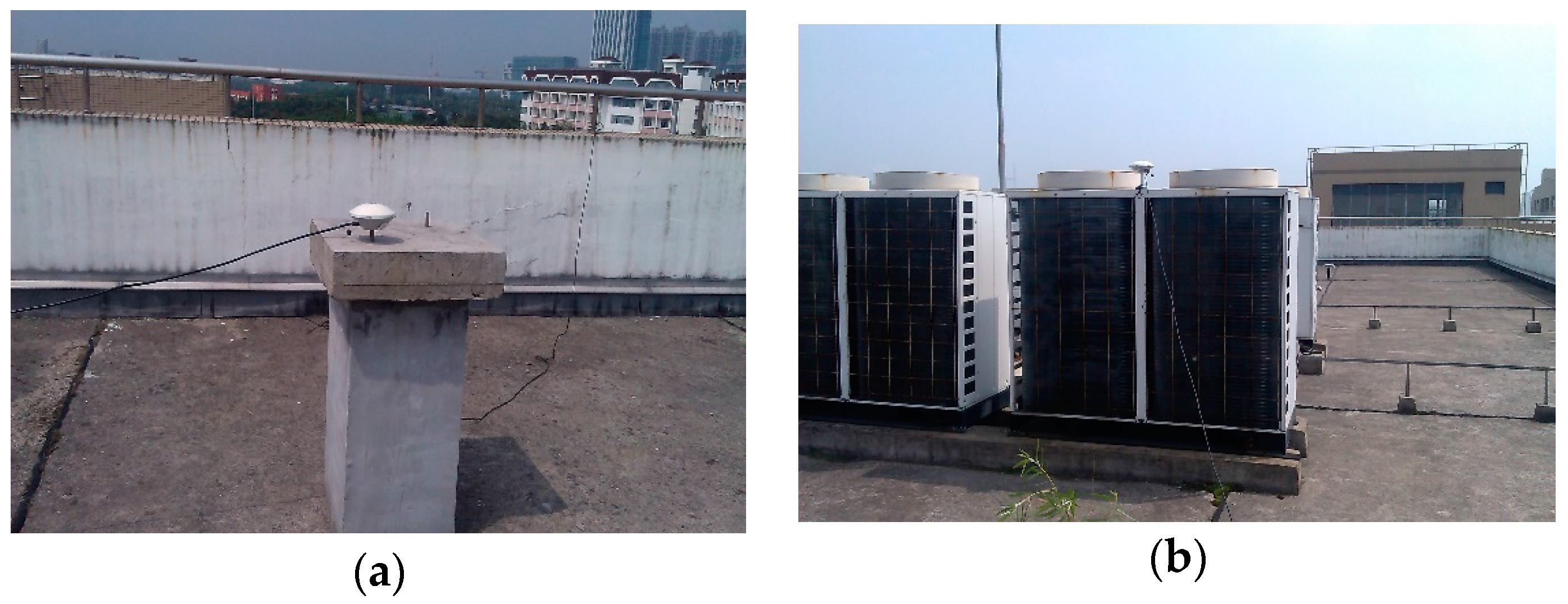
The experimental data for testing RCM were collected from DOY 335 to 354 of 2014. Two antennas were mounted on the roof of a building located at East China Normal University (Figure 3). The baseline length between the two antennas was about 12 m. The two antennas were connected to the same receiver (Trimble BD982 clock synchronization dual-antenna GNSS receiver) [19,20]. During the test, the sampling rate of GPS data collection was set to 1 Hz. We applied the RCM to estimate MRT values for the 20 days. For each satellite, we used the entire residual time series in implementing RCM to ensure that the lengths of the time series were long enough for correlation to generate reliable MRT estimates. The RCM-derived MRT estimates were compared with the ORTM- and ARTA-derived ones for the 20 days.
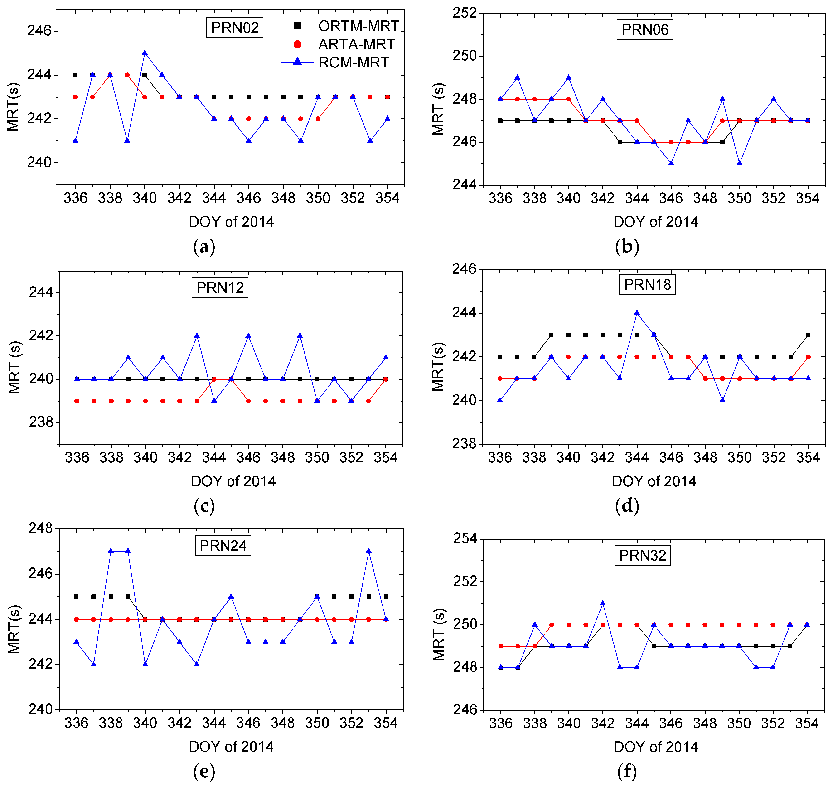
During the period of data collection (DOY 335 to 354 of 2014), the satellite of PRN 13 was undergoing orbit maneuver, and its repeat times were outside the normal range of [86,145, 86,165] s (or [235, 255] s in terms of daily advance time). No other satellites were affected by the maneuver in this period, and their repeat times were within the normal range. We first focused on the MRT estimates of the satellites unaffected by orbit maneuver. The differences between MRT estimates derived by the three methods are mostly not greater than 3 s (Figure 4). The time series of RCM-derived MRT estimates fluctuate more than those derived by the other two methods, and time series of ORTM- and ARTA-derived MRT estimates are closer (Figure 4). Except for the satellite of PRN 13, the absolute values of the differences between MRT estimates derived by ORTM, ARTA, and RCM are calculated for each satellite and each day. The averages of the absolute values of the differences between RCM- and ORTM-derived MRT, between RCM- and ARTA-derived MRT, and between ORTM- and ARTA-derived MRT are 1.18, 1.12 and 0.53 s, respectively.
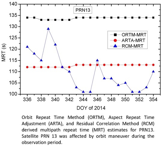
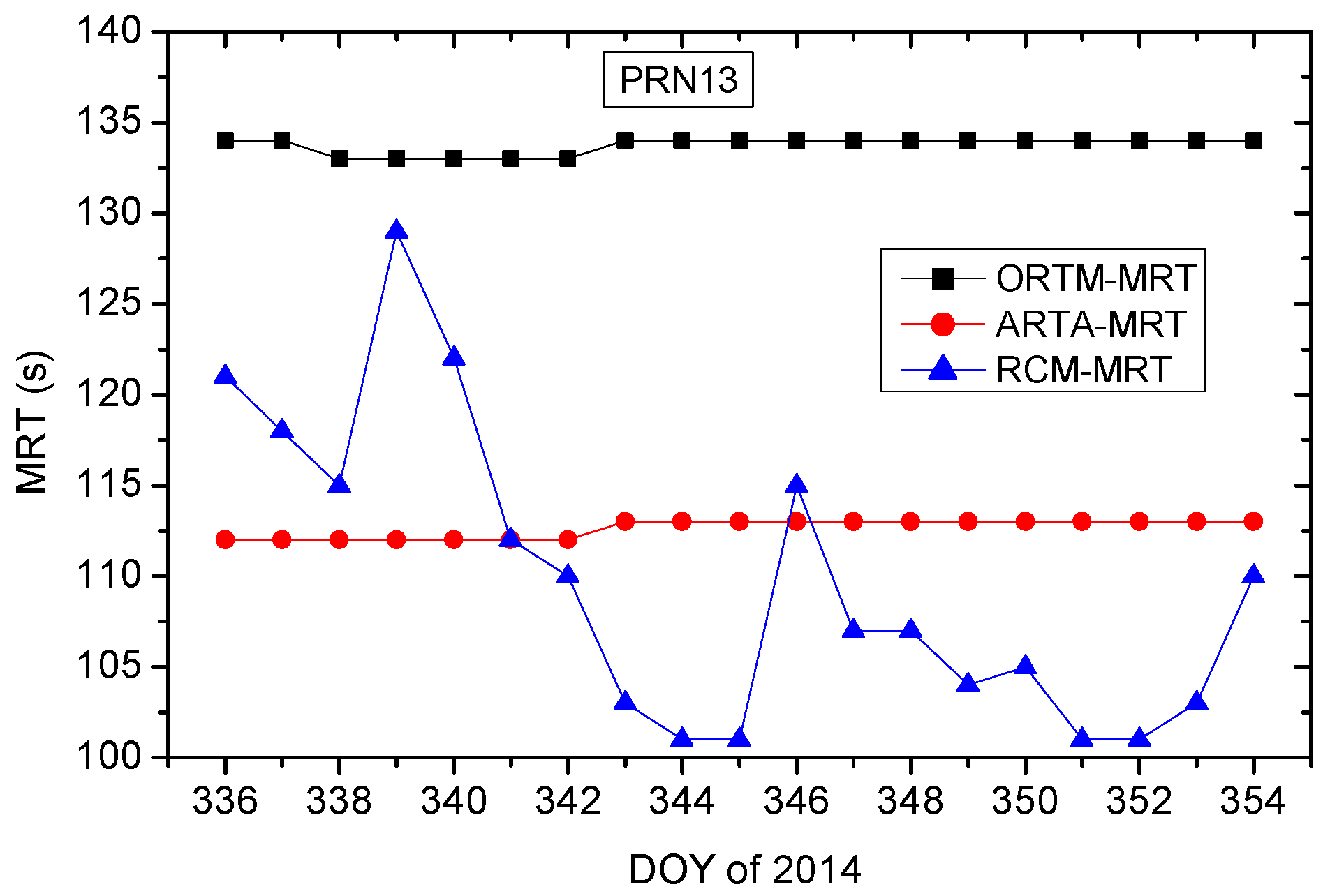
The MRT estimates of PRN 13 derived by the three methods are in the range of 100 to 135 s (Figure 5), which is outside the normal range ([235, 255] s). The time series of ORTM- and ARTA-derived values are relatively stable, with a bias of more than 20 s between them. For the satellite of PRN 13, the time series of RCM-derived MRT estimates fluctuate much more than those derived by the other two methods, and also than the RCM-derived MRT estimates for the other satellites. In comparison, the time series of MRT estimates derived by RCM and ARTA are closer. The contrast of Figure 5 and Figure 4 indicates that the consistency of MRT estimates derived by the three methods decreases significantly when the satellite is affected by orbit maneuver.
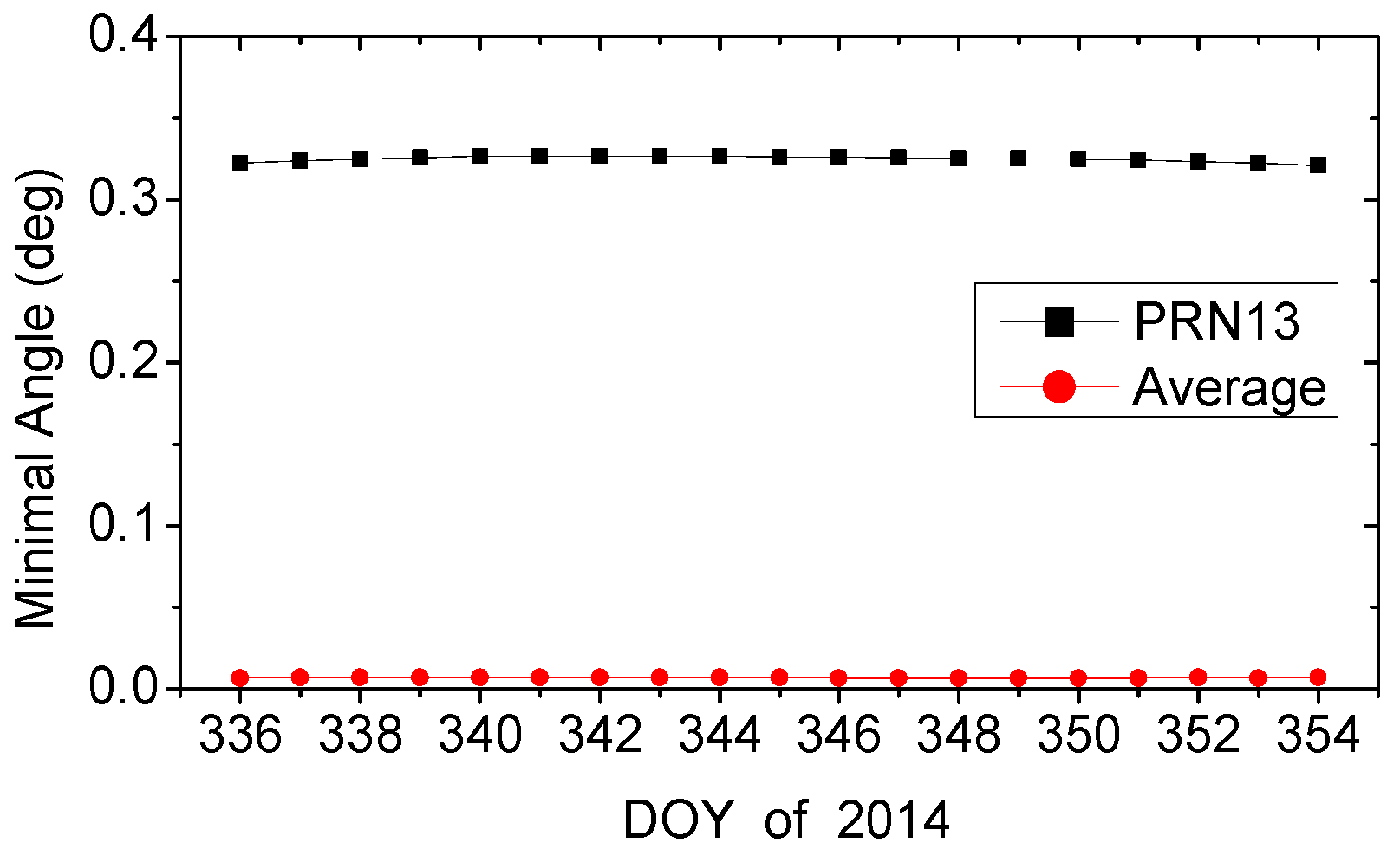
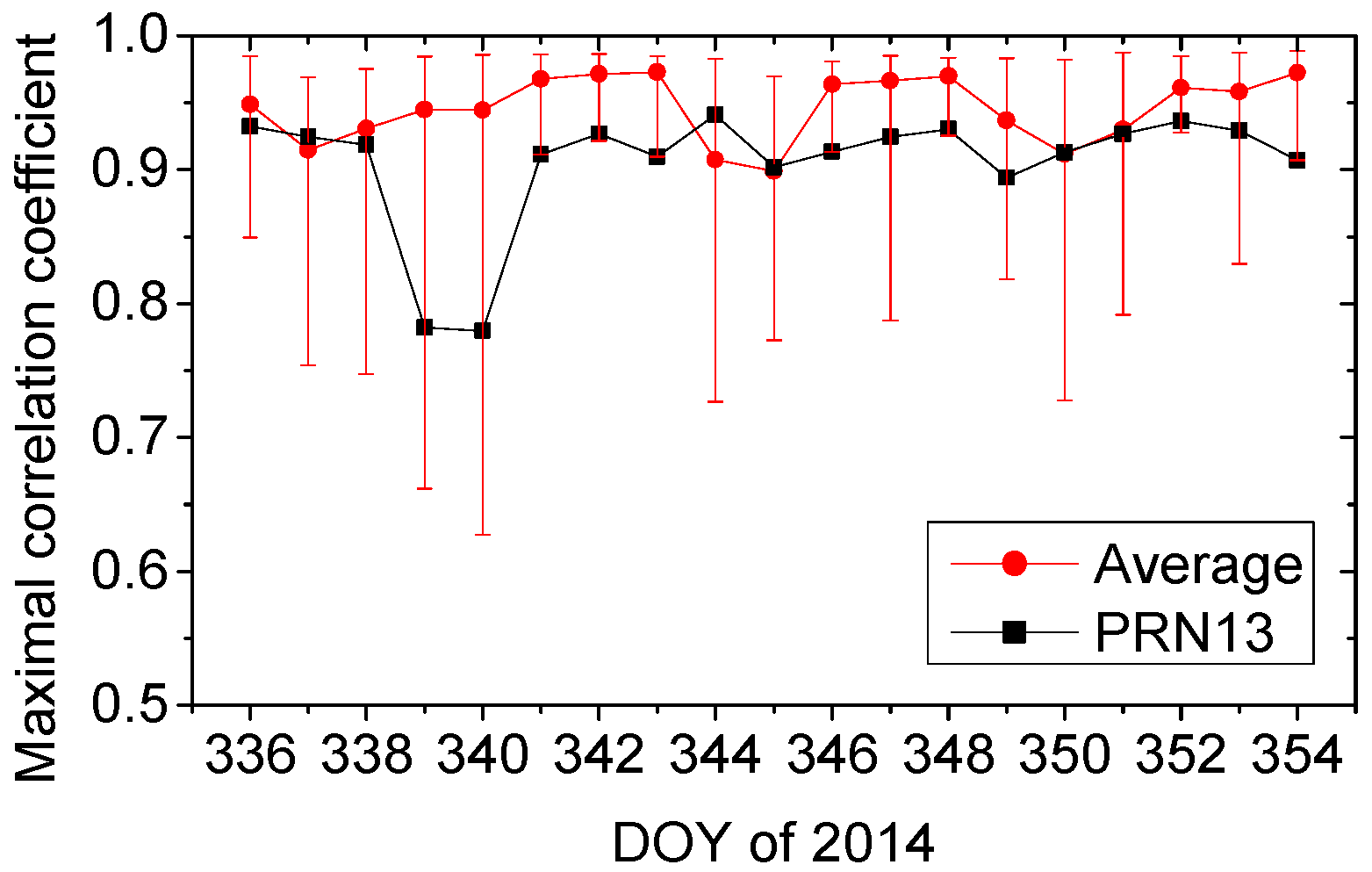
During DOY 336 to 354, 2014, the minimal angles between unit vectors of station-to-satellite from two consecutive days (minimal in ARTA) for PRN13 are about 0.32°, while the averages of minimal angles of other satellites are about 0.07° (Figure 6). Greater minimal angle of PRN13 indicates that the orbit repeatability of the satellite affected by orbit maneuver is weaker than that of unaffected satellites. For PRN13, the maximal correlation coefficients of residual time series from two consecutive days are, in general, a little smaller than the average values for unaffected satellites, but most maximal correlation coefficients for PRN13 are greater than 0.9 (Figure 7), which demonstrates the multipath related to this satellite still repeats well day to day.
3.3. Effectiveness of Multipath Mitigation
MRT estimates derived from the three methods were adopted in ASF, namely ORTM-ASF, ARTA-ASF, and RCM-ASF, to correct the multipath of the single-differenced GPS L1 carrier phase observables, respectively. Then, the three kinds of corrected single-differenced observables were used to estimate the baseline components. For comparison, the uncorrected observables were also used to generate baseline solutions. The time series of the solutions generated from the corrected observables are much more stable than that generated from uncorrected observables (Figure 8), which demonstrates that the three ASF corrections (ORTM-ASF, ARTA-ASF, and RCM-ASF) eliminate multipath effectively.
We estimated the baseline components both with satellite PRN 13 included and excluded, to investigate the influence of the satellite on baseline estimation and on the performance of the three ASF corrections. The results show that the baseline solutions are basically similar, and all the ASF methods perform well, no matter whether PRN 13 is involved in data processing or not (Figure 8), which indicates that the data of PRN13 are usable in baseline estimation and ASF multipath mitigation.
The time series of solutions generated from observables corrected by different ASF methods are very similar on DOY 344, 2014 (Figure 8). This indicates the effectiveness of multipath reduction of the three ASF methods are very close. Time series of solutions of DOY 345 and 346, which are not shown, are similar to that of DOY 344, and will lead to the same conclusions. To distinguish the slight differences between the efficiency of multipath reduction of the three ASF methods, quantitative analysis should be implemented.
STD reduction of baseline component time series is a criterion for assessing the effectiveness of multipath mitigation in coordinate domain. STD of time series of each baseline component for each day was calculated to distinguish slight differences between the time series (Table 1 and Table 2). The STD values were calculated from the data at epochs when the satellite of PRN 13 was visible from the view of the experimental GPS site. Using the observables corrected by the three ASF methods to estimate baseline components, the STD values of time series of the solutions reduce notably comparing to that generated from uncorrected observables (Table 1 and Table 2). When the satellite of PRN 13 is excluded in baseline estimation, STD values of ORTM-ASF are smaller than that of ARTA-ASF in 5 lines, the opposite is true in the other 4 lines (Table 1). Table 1 also shows that STD values of RCM-ASF are smaller than those of the other two methods in 7 lines. The comparisons of STD values indicate that either ORTM-ASF or ARTA-ASF shows no advantage over the other in STD reduction, whereas the RCM-ASF generally performs a little better than the other two methods.
Including PRN 13 in data processing (Table 2), most STD values are smaller than the corresponding ones in Table 1, which indicates that STD values are reduced after adding the satellite of PRN 13 into baseline estimation and multipath corrections. In terms of STD reduction, RCM-ASF still performs better than the other two methods, and the ARTA-ASF shows an obvious advantage over ORTM-ASF (Table 2) contrasting to the comparison of the two methods in Table 1.
The ORTM-ASF performs as well as ARTA-ASF in STD reduction when the satellite PRN 13 is excluded in data processing (Table 1). However, ARTA-ASF performs better than ORTM-ASF when the satellite PRN 13 is included (Table 2). The only explanation for this is the ARTA method derives better MRT estimates than ORTM does for PRN 13. Since the RCM-ASF performs best in both cases of PRN 13 being excluded and included, whether the RCM derives the best MRT estimates for PRN 13 is not clear. For further investigation, the residual time series of single-differenced observables related to PRN 13 were extracted after baseline estimation. The multipath, if not eliminated from the observables, will partly enter into residuals (Figure 9, black line). When the observables are corrected by ORTM-ASF, ARTA-ASF, and RCM-ASF, the time series of residuals extracted after baseline estimation approximate the white noise random time series (Figure 9). RMS of residual time series reflects the level of multipath in residuals, which is a criterion for assessing the effectiveness of multipath mitigation in observation domain. The RMS of residual time series related to satellite PRN 13 were calculated for each day (Table 3). RMS reduction of RCM-ASF is largest for each day, followed by that of ARTA-ASF, and that of ORTM-ASF is the smallest. The comparisons of RMS reduction demonstrate that the MRT estimates of PRN 13 derived by RCM are better than those derived by the other two methods for ASF multipath mitigation.
3.4. Robustness, Computational Cost and Real-Time Application
ORTM and ARTA calculate the MRT estimate at every epoch given by broadcast and precise ephemeris, respectively. The variations between the MRT estimates for the same satellite at different epochs of a day are in general not greater than 2 s; examples are shown in Figure 10. In most cases, MRT estimate derived by ORTM or ARTA at a single epoch is equal or close (less than 2 s) to the daily average value (average of the MRT estimates of all epochs). For RCM, we used different lengths (one hour to seven hours) of residual time series to implement the method for evaluating its robustness; examples are shown in Table 4. The MRT estimates generated from the residual time series of one-hour length may differ by several seconds (up to 10 s), while the differences of MRT estimates generated from that of four-hour length are within 2 s (Table 4). Setting the MRT estimates from the full-length (seven hours) residual time series as the references, four hours is enough long for residual time series to generate MRT estimates with the biases (to references) less than three seconds.
ORTM reads only two parameters ( and ) from broadcast ephemeris to calculate the repeat time of individual satellite with a very simple formula. This method has the lowest computational cost of the three. ARTA reads satellite positions from IGS precise ephemeris and calculates the unit vector of line-of-sight of station-to-satellite. In addition, there is a searching process in ARTA, which is time-consuming. Thus, the ARTA takes more computation than ORTM. RCM also includes a searching process. Besides, the residual time series have to be generated in advance for implementing RCM, which costs extra time. Hence the computational cost of RCM is the highest of the three.
As for real-time ASF, ARTA is an appropriate choice. IGS ultra-rapid ephemeris contains 24 h of predicted orbit. By adopting ultra-rapid ephemeris, ARTA is able to predict the MRT for the next day, which makes ARTA adaptable for real-time ASF. MRT estimates for each satellite (focus on satellite unaffected by orbit maneuvering) and each day of 2014 and 2015 were calculated by using IGS final and ultra-rapid ephemerides, respectively. MRT estimates generated from IGS final and ultra-rapid ephemerides are exactly the same for the majority of estimated values (Table 5), which suggests that ARTA in real-time mode generates almost the same MRT estimates as does it in post-processing mode.
4. Discussion
For satellites unaffected by orbit maneuvering, the MRT estimates derived by the three methods are very close. Our results show that the average of the differences between MRT estimates derived by ORTM and ARTA is less than one second, which is consistent with the results of Fang [10] and Agnew and Larson [16]. From the DOY of 335 to 354, 2014, the averages of the differences between RCM-derived MRT estimates and the other two methods derived ones are less than 1.2 s. In the case of all the adopted satellites are unaffected by orbit maneuvering, the multipath reductions are basically identical when the MRT estimates from the three methods are adopted by ASF to eliminate multipath. In comparison, RCM-derived MRT estimates show a slight advantage in multipath reduction.
Satellite PRN 13 was affected by orbit maneuvering during the observation period. The consistencies of the time series of MRT estimates from the three methods for PRN 13 are not as high as those for the unaffected satellites. There is a bias of about 20 s between the time series of MRT estimates from ORTM and ARTA for PRN 13. The time series of RCM-derived MRT estimates fluctuate much more for PRN 13 than for other unaffected satellites. The differences of multipath reduction of the three methods are more notable when PRN 13 was included in data processing. ORTM only uses orbit data and the method in nature calculates the orbit period of individual satellite. ARTA uses orbit data and the coordinates of a selected GPS station, and it calculates the repeat time of the geometric relationships between station and satellites. Larson et al. [8] pointed out that ARTA-derived estimates are better for representing real MRT than ORTM-derived ones. For PRN 13, our results show that using ARTA-derived MRT estimates in ASF eliminates multipath more effectively than using estimates derived by ORTM, which confirms the viewpoint of Larson et al. [8].
RCM uses both orbit and observation data. The residual time series used in RCM are generated from the orbit and observation data, which contain the real multipath errors. If the other noises in the residual time series are eliminated, the method of searching maximal correlation coefficients between residual time series of two consecutive days is expected to generate the best MRT estimates of the three methods. Comparisons of multipath reductions of the three methods verify this expectation. The comparisons indicate that adopting the MRT estimates derived by RCM in implementing ASF performs better than adopting that from the other methods for multipath mitigation, no matter PRN 13 is included or not.
Previous studies did not adopt the data of satellites affected by orbit maneuvering in data processing (e.g., [6,9,11,13]). Choi et al. [6] and Larson et al. [8] used the mean MRT of the adopted satellites to implement sidereal filtering, and the effectiveness of multipath mitigation will get worse if the data of the affected satellites are included in their sidereal filtering. The ASF treats the observables of each satellite separately, thus the MRT estimate of one satellite deviating from the normal range does not affect the multipath mitigation for the observables of other satellites. We compared the STD of the time series of the baseline components estimated with and without PRN 13. The effectiveness of multipath elimination is not affected remarkably when PRN 13 is included in multipath mitigation and baseline estimation (contrasting Table 1 and Table 2), which indicates that the data of satellite affected by orbit maneuvering can be used in sidereal filter as long as the filter treats the data of each satellite separately.
Though this study focuses on calculating MRT of GPS satellites, the three methods can be adapted to derive the repeat time of other GNSS constellations. Since the repeat time of other GNSS satellite may be no longer near a sidereal day, the methods should be implemented with caution when they are used for the non-GPS systems. For example, the GLONASS satellites run 17 revolutions in 8 days and hence the MRT of GLONASS satellite is near 8 days [23]. To eliminate the multipath of GLONASS satellites for the day of interest, we should use the residual time series from eight days ago to generate multipath correction model rather than from one day before. For GLONASS, the orbit data (residual time series) from two days with the interval of eight days are adopted by ARTA (RCM) to derive the MRT estimates. Using the ORTM for GLONASS, Equation (3) should be modified to 17 orbit periods instead of 2 orbit periods. The medium earth orbit satellites of BDS (BeiDou navigation satellite system) run 13 revolutions in 7 days [24] and the GALILEO satellites run 17 cycles in 10 days [1]. Similarly, the three methods should be adjusted accordingly when they are used for these two navigation satellite systems.
5. Conclusions
Multipath mitigation is an important step in GNSS data processing for geodetic and geophysical applications. The success of multipath elimination improves the precision and accuracy of GNSS positioning, which also contributes to the extraction of geophysical signals from the time series of GNSS solutions. Sidereal filtering can mitigate the GPS multipath effectively. However, without adopting accurate MRT in implementing sidereal filtering may well result in poorer multipath reduction. There are three commonly-used methods (ORTM, ARTA, and RCM) to estimate accurate MRT for improving sidereal filtering. We analyzed the robustness of the three methods. For ORTM and ARTA, in most cases, MRT estimates generated from the orbit data of a single epoch are equal or close (difference less than two seconds) to daily average MRT values for GPS satellites. For RCM, the length of residual time series may affect the MRT estimates, adopting the length of four hours or more is suggested to generate stable MRT estimates.
We compared the three methods in terms of efficiency of multipath mitigation, computational cost, and adaptability for real-time application, in order to provide a basis for method selection in practical applications. The RCM derives best MRT estimates for multipath mitigation no matter the satellite is affected by orbit maneuvering or not, though its advantage in multipath reduction over the other two methods is not significant (Table 1 and Table 2). Thus, if the aim is to achieve the maximal multipath reduction, RCM is the right choice. ORTM is easy to implement and has the lowest computational cost among the three methods. As to real-time application, ARTA is the best choice because this method can utilize ultra-rapid orbit ephemerides of IGS to estimate MRT for the coming day. For a satellite affected by orbit maneuvering, the MRT estimates derived by ARTA and RCM are better than that derived by ORTM in multipath reduction. Thus, we suggest choosing ARTA or RCM in preference to ORTM for the case of affected satellite(s) being involved in multipath mitigation.
Acknowledgments
We are very grateful to the three anonymous reviewers for their constructive comments and suggestions. This research is sponsored by National Key R&D Program of China (No. 2017YFE0100700), National Natural Science Foundation of China (No. 41771475), and National Basic Research Program of China (No. 2013CB733314). Availability of Data: The orbit data used in this study can be downloaded from the data center of SOPAC and CDDIS. The observation data collected by dual-antenna GNSS receiver and the source codes of multipath repeat time calculating methods are available on request basis to the first author, Minghua Wang ([email protected]).
Author Contributions
Minghua Wang, Jiexian Wang, and Danan Dong conceived and designed the experiments; Minghua Wang and Haojun Li performed the experiments and analyzed the data; Ling Han and Wen Chen contributed analysis tools; Minghua Wang wrote the paper; All authors read and approved the final manuscript.
Conflicts of Interest
The authors declare no conflict of interest.
Abbreviations
| GNSS | Global Navigation Satellite System |
| GPS | Global Positioning System |
| GLONASS | Globalnaya navigatsionnaya sputnikovaya Sistema |
| BDS | BeiDou Navigation Satellite System |
| GALILEO | Galileo Navigation Satellite System |
| MRT | Multipath Repeat Time |
| ORTM | Orbit Repeat Time Method |
| ARTA | Aspect Repeat Time Adjustment |
| RCM | Residual Correlation Method |
| ASF | Advanced Sidereal Filtering |
| DOY | Day of Year |
| N, E, and U | North, East, and Up |
| PRN | Pseudo Random Noise Code Number |
| STD | Standard Deviation |
| RMS | Root Mean Square |
| IGS | International GNSS Service |
| SOPAC | Scripps Orbit and Permanent Array Center |
| CDDIS | Crustal Dynamics Data Information System |
References
- Hofmann-Wellenhof, B.; Lichtenegger, H.; Wasle, E. GNSS—Global Naviagtion Satellite System; Springer: Vienna, Austria, 2008; pp. 154–155. ISBN 978-3-211-73012-6. [Google Scholar]
- Park, K.; Nerem, R.; Schenewerk, M.; Davis, J. Site-specific multipath characteristics of global IGS and CORS GPS sites. J. Geod. 2004, 77, 799–803. [Google Scholar] [CrossRef]
- Bock, Y. Continuous monitoring of crustal deformation. GPS World 1991, 2, 40–47. [Google Scholar]
- Genrich, J.; Bock, Y. Rapid resolution of crustal motion at short ranges with the Global Positioning System. J. Geophys. Res. 1992, 97, 3261–3269. [Google Scholar] [CrossRef]
- Wübbena, G.; Schmitz, M.; Menge, F.; Seeber, G.; Völksen, C. A new approach for field calibration of absolute GPS antenna phase center variations. Navigation 1997, 44, 247–255. [Google Scholar] [CrossRef]
- Choi, K.; Bilich, A.; Larson, K.; Axelrad, P. Modified sidereal filtering: Implications for high-rate GPS positioning. Geophys. Res. Lett. 2004, 31, L22608. [Google Scholar] [CrossRef]
- Yin, H.; Gan, W.; Xiao, G. Modified sidereal filter and its effect on high-rate GPS positioning. Geomat. Inf. Sci. Wuhan Univ. 2011, 36, 609–611. [Google Scholar]
- Larson, K.; Bilich, A.; Axelrad, P. Improving the precision of high-rate GPS. J. Geophys. Res. 2007, 112, B05422. [Google Scholar] [CrossRef]
- Ragheb, A.; Clarke, P.; Edwards, S. GPS sidereal filtering: Coordinate and carrier-phase-level strategies. J. Geod. 2007, 81, 325–335. [Google Scholar] [CrossRef]
- Fang, R. High-Rate GPS Data Non-Difference Precise Processing and Its Application on Seismology. Ph.D. Thesis, Wuhan University, Wuhan, China, 2010. [Google Scholar]
- Zhong, P.; Ding, X.; Yuan, L.; Xu, Y.; Kwok, K.; Chen, Y. Sidereal filtering based on single differences for mitigating GPS multipath effects on short baselines. J. Geod. 2010, 84, 145–158. [Google Scholar] [CrossRef]
- Lau, L. Comparison of measurement and position domain multipath filtering techniques with the repeatable GPS orbits for static antennas. Surv. Rev. 2012, 44, 9–16. [Google Scholar] [CrossRef]
- Atkins, C.; Ziebart, M. Effectiveness of observation-domain sidereal filtering for GPS precise point positioning. GPS Solut. 2016, 20, 111–122. [Google Scholar] [CrossRef]
- Zheng, D.; Zhong, P.; Ding, X.; Chen, W. Filtering GPS time-series using a Vondrak filter and cross validation. J. Geod. 2005, 79, 363–369. [Google Scholar] [CrossRef]
- Shen, F.; Li, J.; Zhang, X.; Shu, C. The improved sidereal filtering of time series considering segments’ similarity in coseismic displacement. Acta Geod. Cartogr. Sin. 2013, 42, 487–492. [Google Scholar]
- Agnew, D.; Larson, K. Finding the repeat times of the GPS constellation. GPS Solut. 2007, 11, 71–76. [Google Scholar] [CrossRef]
- Axelrad, P.; Larson, K.; Jones, B. Use of the correct satellite repeat period to characterize and reduce site-specific multipath errors. In Proceedings of the ION GNSS 2005, Long Beach, CA, USA, 13–16 September 2005; pp. 2638–2648. [Google Scholar]
- Dong, D.; Wang, M.; Chen, W.; Zeng, Z.; Song, L.; Zhang, Q.; Cai, M.; Cheng, Y.; Lv, J. Mitigation of multipath effect in GNSS short baseline positioning by the multipath hemispherical map. J. Geod. 2016, 90, 255–262. [Google Scholar] [CrossRef]
- Dong, D.; Chen, W.; Cai, M.; Zhou, F.; Wang, M.; Yu, C.; Zheng, Z.; Wang, Y. Multi-antenna synchronized global navigation satellite system receiver and its advantages in high-precision positioning applications. Front. Earth Sci. 2016, 4, 772–783. [Google Scholar] [CrossRef]
- Cai, M.; Chen, W.; Dong, D.; Song, L.; Wang, M.; Wang, Z.; Zhou, F.; Zheng, Z.; Yu, C. Reduction of Kinematic Short Baseline Multipath Effects Based on Multipath Hemispherical Map. Sensors 2016, 16, 1677. [Google Scholar] [CrossRef] [PubMed]
- Wang, M.; Wang, J.; Dong, D.; Chen, W. Detecting and repairing cycle-slip for clock-synchronized dual-antenna global positioning system data based on single-differencing between antennas. J. Tongji Univ. Nat. Sci. 2016, 44, 462–468. [Google Scholar]
- Chen, W.; Yu, C.; Dong, D.; Cai, M.; Zhou, F.; Wang, Z.; Zhang, L.; Zheng, Z. Formal uncertainty and dispersion of single and double difference models for GNSS-based attitude determination. Sensors 2017, 17, 408. [Google Scholar] [CrossRef] [PubMed]
- Geng, J.; Jiang, P.; Liu, J. Integrating GPS with GLONASS for high-rate seismogeodesy. Geophys. Res. Lett. 2017, 44, 3139–3146. [Google Scholar] [CrossRef]
- Ye, S.; Chen, D.; Liu, Y.; Jiang, P.; Tang, W.; Xia, P. Carrier phase multipath mitigation for BeiDou navigation satellite system. GPS Solut. 2015, 19, 545–557. [Google Scholar] [CrossRef]
Figure 1.
Flowchart of the comparison of MRT estimates derived by ORTM, ARTA, and RCM.

Figure 2.
Comparison of ORTM- and ARTA-derived MRT estimates. AVDOA is short for “the absolute value of the difference between ORTM- and ARTA-derived MRT”. The y-axis, showing “percentage of AVDOA no larger than 2 s”, is on the right side of the upper panel.
Figure 2.
Comparison of ORTM- and ARTA-derived MRT estimates. AVDOA is short for “the absolute value of the difference between ORTM- and ARTA-derived MRT”. The y-axis, showing “percentage of AVDOA no larger than 2 s”, is on the right side of the upper panel.

Figure 3.
Set-up of the data collection at East China Normal University. Two antennas connect to the same GNSS receiver. (a) One antenna mounted on a concrete pillar (Latitude: 31.035631°N; Longitude: 121.444421°E); (b) the other antenna set on the top of an A/C compressor (Latitude: 31.035640°N; Longitude: 121.444550°E).

Figure 4.
ORTM-, ARTA-, and RCM-derived MRT estimates for PRN 02, 06, 12, 18, 24, and 32. The y-axes denote the daily advance time. MRT estimate equals 86,400 s minus daily advance time. Legend shown on (a) is for the all (a–f).
Figure 4.
ORTM-, ARTA-, and RCM-derived MRT estimates for PRN 02, 06, 12, 18, 24, and 32. The y-axes denote the daily advance time. MRT estimate equals 86,400 s minus daily advance time. Legend shown on (a) is for the all (a–f).

Figure 5.
ORTM-, ARTA-, and RCM-derived MRT estimates for PRN13. The y-axis shows the daily advance time. MRT estimate equals 86,400 s minus daily advance time.
Figure 5.
ORTM-, ARTA-, and RCM-derived MRT estimates for PRN13. The y-axis shows the daily advance time. MRT estimate equals 86,400 s minus daily advance time.

Figure 6.
Minimal angle (minimal value in ARTA) between receiver-to-satellite unit vectors of each two consecutive days from DOY 335 to 354, 2014. The black squares are the minimal angles for PRN 13; each value is a daily average. The red circles are the average minimal angles of all the satellites with the repeat time in the normal range.

Figure 7.
Maximal correlation coefficients (in RCM) of residual time series of each two consecutive days from DOY 335 to 354, 2014. The black squares are the maximal correlation coefficients for PRN 13. The red circles are the average maximal correlation coefficients of all the satellites with the repeat time in the normal range; the upper bound is the maximum of maximal correlation coefficients of all the satellites for each day; the lower bound is the minimum of that for each day.

Figure 8.
Baseline components estimated from the observables with ORTM-ASF correction, with ARTA-ASF correction, with RCM-ASF correction, and without any ASF correction for DOY 344, 2014. (a,c,e) are N, E, and U components estimated with satellite of PRN 13 excluded. (b,d,f) are N, E, and U components estimated with satellite of PRN 13 included. For comparison, time series of “ORTM-ASF”, “ARTA-ASF”, and “RCM-ASF” are shifted by −3, −6, and −9 cm for N and E, and by −5, −10, and −15 cm for U. Legend shown on (a) is for all of (a–f). The time series are shown from epoch 7130 to epoch 26,681, when the data of satellite PRN 13 were receivable.

Figure 9.
Residual time series of single-differenced observables for PRN 13 on DOY 344, 2014. For comparison, time series of “ORTM-ASF”, “ARTA-ASF”, and “RCM-ASF” are shifted by −1.5, −3, and −4.5 cm, respectively.
Figure 9.
Residual time series of single-differenced observables for PRN 13 on DOY 344, 2014. For comparison, time series of “ORTM-ASF”, “ARTA-ASF”, and “RCM-ASF” are shifted by −1.5, −3, and −4.5 cm, respectively.

Figure 10.
MRT estimates for PRN02 and PRN16 on DOY 344, 2014. (a) MRT estimates derived (every two hours) by ORTM; (b) MRT estimates derived (every hour) by ARTA.
Figure 10.
MRT estimates for PRN02 and PRN16 on DOY 344, 2014. (a) MRT estimates derived (every two hours) by ORTM; (b) MRT estimates derived (every hour) by ARTA.


Table 1.
STD of time series of baseline components estimated from observables with and without ASF correction (Excluding PRN 13).
Table 1.
STD of time series of baseline components estimated from observables with and without ASF correction (Excluding PRN 13).
| DOY | Baseline Component | STD (mm) | |||
|---|---|---|---|---|---|
| Without ASF | With ASF | ||||
| ORTM-ASF | ARTA-ASF | RCM-ASF | |||
| 344 | N | 4.2539 | 2.0367 | 2.0385 | 2.0381 |
| E | 2.9165 | 1.5699 | 1.5719 | 1.5712 | |
| U | 6.6746 | 4.0606 | 4.0624 | 4.0604 | |
| 345 | N | 4.8240 | 2.4629 | 2.4626 | 2.4625 |
| E | 3.1866 | 1.9315 | 1.9305 | 1.9301 | |
| U | 8.8673 | 5.2794 | 5.2761 | 5.2704 | |
| 346 | N | 4.8628 | 2.5575 | 2.5555 | 2.5512 |
| E | 3.0163 | 1.7367 | 1.7372 | 1.7365 | |
| U | 7.8131 | 5.1112 | 5.1134 | 5.1047 | |
Table 2.
STD of time series of baseline components estimated from observables with and without ASF correction (Including PRN 13).
Table 2.
STD of time series of baseline components estimated from observables with and without ASF correction (Including PRN 13).
| DOY | Baseline Component | STD (mm) | |||
|---|---|---|---|---|---|
| Without ASF | With ASF | ||||
| ORTM-ASF | ARTA-ASF | RCM-ASF | |||
| 344 | N | 3.5171 | 1.9142 | 1.8862 | 1.8857 |
| E | 2.8904 | 1.5855 | 1.5613 | 1.5603 | |
| U | 6.6472 | 4.0482 | 3.9842 | 3.9844 | |
| 345 | N | 4.0800 | 2.2783 | 2.2551 | 2.2548 |
| E | 3.0700 | 1.8916 | 1.8656 | 1.8641 | |
| U | 8.7254 | 5.0073 | 4.9048 | 4.8928 | |
| 346 | N | 4.0967 | 2.2461 | 2.2303 | 2.2264 |
| E | 2.9853 | 1.6951 | 1.6768 | 1.6756 | |
| U | 7.8988 | 4.7870 | 4.7254 | 4.7196 | |
Table 3.
RMS of residual time series for PRN 13.
| DOY | RMS (mm) | |||
|---|---|---|---|---|
| Without ASF | With ASF | |||
| ORTM-ASF | ARTA-ASF | RCM-ASF | ||
| 344 | 3.5947 | 1.8189 | 1.7951 | 1.7940 |
| 345 | 3.4139 | 1.8683 | 1.8427 | 1.8397 |
| 346 | 2.9936 | 1.7128 | 1.6926 | 1.6919 |
Table 4.
MRT estimates derived by RCM with different length of residual time series for PRN02 and PRN16 on DOY 344, 2014. The full lengths of residual time series of PRN02 and PRN16 are about 7.1 h.
Table 4.
MRT estimates derived by RCM with different length of residual time series for PRN02 and PRN16 on DOY 344, 2014. The full lengths of residual time series of PRN02 and PRN16 are about 7.1 h.
| PRN | Length of Residual Time Series for Correlation | ||||||
|---|---|---|---|---|---|---|---|
| 1 h | 2 h | 3 h | 4 h | 5 h | 6 h | 7 h | |
| PRN02 | 242 | 242 | 242 | 242 | 242 | 241 | 242 |
| 242 | 242 | 242 | 241 | 241 | 242 | ||
| 243 | 241 | 239 | 240 | 241 | |||
| 240 | 237 | 239 | 241 | ||||
| 235 | 239 | 242 | |||||
| 241 | 243 | ||||||
| 244 | |||||||
| PRN16 | 240 | 240 | 241 | 241 | 242 | 242 | 243 |
| 241 | 242 | 242 | 243 | 243 | 243 | ||
| 243 | 243 | 244 | 243 | 243 | |||
| 242 | 245 | 243 | 243 | ||||
| 246 | 244 | 243 | |||||
| 242 | 242 | ||||||
| 242 | |||||||
Table 5.
The distribution of the differences between MRT estimates derived from IGS final and ultra-rapid ephemerides using ARTA. The ‘Difference’ in column one is MRT estimate derived from IGS final ephemeris minus that derived from IGS ultra-rapid ephemeris for each satellite and for each day of 2014 and 2015.
| Difference (s) | Number |
|---|---|
| −4 | 2 |
| −3 | 0 |
| −2 | 2 |
| −1 | 1 |
| 0 | 21,348 |
| 1 | 2 |
| 2 | 3 |
© 2018 by the author. Licensee MDPI, Basel, Switzerland. This article is an open access article distributed under the terms and conditions of the Creative Commons Attribution (CC BY) license (http://creativecommons.org/licenses/by/4.0/).
Share and Cite
MDPI and ACS Style
Wang, M.; Wang, J.; Dong, D.; Li, H.; Han, L.; Chen, W. Comparison of Three Methods for Estimating GPS Multipath Repeat Time. Remote Sens. 2018, 10, 6. https://doi.org/10.3390/rs10020006
AMA Style
Wang M, Wang J, Dong D, Li H, Han L, Chen W. Comparison of Three Methods for Estimating GPS Multipath Repeat Time. Remote Sensing. 2018; 10(2):6. https://doi.org/10.3390/rs10020006
Chicago/Turabian StyleWang, Minghua, Jiexian Wang, Danan Dong, Haojun Li, Ling Han, and Wen Chen. 2018. "Comparison of Three Methods for Estimating GPS Multipath Repeat Time" Remote Sensing 10, no. 2: 6. https://doi.org/10.3390/rs10020006
Note that from the first issue of 2016, this journal uses article numbers instead of page numbers. See further details here.