The Impacts of the Ionospheric Observable and Mathematical Model on the Global Ionosphere Model

Abstract

A high-accuracy Global Ionosphere Model (GIM) is significant for precise positioning and navigating with the Global Navigation Satellite System (GNSS), as well as space weather applications. To obtain a precise GIM, it is critical to take both the ionospheric observable and mathematical model into consideration. In this contribution, the undifferenced ambiguity-fixed carrier-phase ionospheric observable is first determined from a global distribution of permanent receivers. Accuracy assessment with a co-located station experiment shows that the observational errors affecting the ambiguity-fixed carrier-phase ionospheric observables range from 0.10 to 0.35 Total Electron Content Units (TECUs, where 1 TECU $={10}^{16}{\mathrm{e}}^{-}/{\mathrm{m}}^2$ and corresponds to 0.162 m on the Global Positioning System, GPS L1 frequency), indicating that the ambiguity-fixed carrier-phase ionospheric observable is over one order of magnitude more accurate than the carrier-phase leveled-code one (from 1.21 to 3.77 TECUs). Second, to better model the structure of the ionosphere, a two-layer GIM has been built based on the above carrier-phase observable. Preliminary global accuracy evaluation demonstrates that the accuracy of the two-layer GIM is below 1 TECU and about 2 TECUs during low and high solar activity periods. Third, the single-frequency point positioning experiment is adopted to test the ionosphere mitigation effects of the GIMs. Positioning results demonstrate that the single-frequency positioning accuracy can be improved by more than 30% using the undifferenced ambiguity-fixed ionospheric observable-derived two-layer GIM, compared with that using the carrier-phase leveled-code ionospheric observable-based single-layer GIM.

1. Introduction

The ionosphere can be defined as the part of the upper atmosphere, between 60 and 2000 km in height, where the density of free electrons and ions is high enough to influence the propagation of electromagnetic radio frequency waves [1]. When electromagnetic signals pass through the ionosphere, the signal path will undergo bending and the propagation velocity will be changed (mainly affected by free electrons). This ionospheric delay is still one of the main error sources when positioning and navigating with Global Navigation Satellite System (GNSS). Reliable modeling of the propagation errors in the ionosphere is essential to accelerate the integer Ambiguity Resolution (AR) in Precise Point Positioning (PPP) [2,3,4,5,6,7,8] and even enable the GLONASS (GLObal NAvigation Satellite System; Russian Federal Space Agency, Moscow, Russia) PPP-AR, where ionosphere corrections are required to fix ambiguities across inhomogeneous stations. Besides, the ionospheric information is also important in the network Real Time Kinematic (RTK) positioning technique, and also static positioning over longer baselines [9,10]. Furthermore, related scientific studies of the ionosphere (e.g., ionospheric storms, ionospheric scintillation, and anomalous variations of geomagnetic storms, earthquakes and tsunamis) also require permanent and continuous monitoring of the ionospheric state [11,12,13,14,15,16,17]. Therefore, how to obtain a precise Global Ionospheric Model (GIM) is an important issue for precise positioning and space weather applications.

The first essential task to build a precise ionosphere model is to extract the ionospheric observable from the GNSS code and carrier-phase observations [18]. The carrier-phase to code-leveling process [19,20,21] is widely used to extract the ionospheric observable in the GNSS ionosphere research community, for example in the routine calculations of the Ionosphere Associate Analysis Centers (IAACs) in the context of IGS (International GNSS service) Ionosphere Working Group (IIWG), such as ESOC (European Space Operations Center of European Space Agency, ESA, Darmstadt, Germany), JPL (Jet Propulsion Laboratory, Pasadena, CA, USA) and NRCan (National Resources Canada, Canada, resumed since April 2015) [22,23]. The carrier-phase leveled to code-delay ionospheric observable (or so-called smoothed pseudo-range geometry-free combination, “SP4” for short hereafter) takes advantage of the unambiguous pseudo-range and precise carrier-phase measurement. By averaging the difference between the carrier phase and code delay per continuous arc (i.e., the continuous epochs between a cycle slip or a loss of lock), the unknown ambiguity term can be estimated. Its simplicity and effectiveness make it preferred by most of the IAACs. However, as reported in [24], the accuracy of SP4 observable is affected by leveling errors, which mainly are the code multipath effect, ranging from 1.4 to 5.3 TECUs (Total Electron Content Units). This motivated us to improve the accuracy of the ionospheric observable further.

Recently, geodetic processing, mainly based on a network solution [25] or precise point positioning technique [26], has gained the interest of many researchers for deriving the ionospheric observable [25,26,27,28,29,30,31]. In fact, the carrier-phase measurement is two orders of magnitude more accurate than the code-delay one [32,33]. Unfortunately, it is affected by the ambiguity term. To deal with that, the network-based geodetic processing maps the fixed double-differenced ambiguities to the undifferenced integer ambiguities while in the case of PPP, the ambiguity term is estimated through accurate modeling, using precise orbit and clock products from IGS [34,35,36,37]. Substituting the fixed undifferenced ambiguity term into the carrier-phase geometry-free combination, the Slant Total Electron Content (STEC) can then be retrieved from the undifferenced ambiguity-fixed carrier-phase ionospheric observable (or called “FL4” hereafter).

After the retrieval of the STEC, the STEC is modeled to the Vertical TEC (VTEC), especially for the use of the single-frequency users. The accuracy of the ionospheric models depends on how well the mathematical model can fit the structure of the ionosphere on a global or regional scale during some period of time. Among others, Spherical Harmonic (SH), POLYnomial (POLY) and Generalized Trigonometric Series Function (GTSF) models are commonly used in regional and global ionosphere modeling [23,38]. For example, the SH model with 15 degrees plus 15 orders is employed by IAACs, such as CODE (Center for Orbit Determination in Europe, Bern, Switzerland), and the aforementioned ESOC and NRCan. The model error of the SH model is typically 2 to 8 TECUs [23]. One of the factors limiting the accuracy of the GIMs is the use of the single-layer model. In fact, the ionosphere can be separated into two main components: the ionosphere and plasmasphere. The two components have different height distributions and dynamic evolutions [30]. Therefore, a two-layer GIM has been built and then evaluated in this paper.

The paper is organized as follows. Section 2 summarizes the methodology of STEC retrieval from different ionospheric observables and VTEC modeling. Besides, the methods to assess the accuracy of the ionospheric observable and ionosphere model are described. Section 3 presents the numerical results of the accuracy evaluation of the ionospheric observable and GIMs, additionally with the single-frequency positioning experiment test. Section 4 discusses the positioning results in relation to the accuracy of the ionospheric observable and ionosphere model. Finally, Section 5 summarizes the results and gathers the conclusions.

2. Methodology

2.1. Slant Total Electron Content Retrieval

The raw code and carrier-phase ionospheric observable are shown as below. Note the change in the order of terms in code ionospheric observable $P_I$ and carrier-phase ionospheric observable $L_I$ (i.e., the ionospheric range delay for code observations has opposite sign than for carrier-phase).

$$P_I=P_2-P_1=I+K_{21}+{\epsilon }_{P_I}$$

(1)

$$L_I={\Phi }_1-{\Phi }_2=I+K_{21}+(b_1-b_2)+({\lambda }_1{N}_1-{\lambda }_2{N}_2)+{\epsilon }_{{\Phi }_I}$$

(2)

where $P_f,{\Phi }_f$ are the pseudo-range and carrier-phase measurements (m) at frequency $f$ (Hz), $K_{21}$ is the sum of the satellite and receiver code instrumental delays (or called DCB, in meters), ${\lambda }_f$ is the wavelength (m) and $N_f$ the integer ambiguity (cycle) at frequency $f$, $b_f$ is a frequency-dependent bias (m), $\epsilon$ (m) is the combination of the measurements noise and multipath distinguishing the pseudo-range ${\epsilon }_P$ from the carrier-phase ${\epsilon }_{\Phi }$.

Besides, $I$ is defined as the ionospheric delay in the geometry-free combination as

$$I=({\alpha }_2-{\alpha }_1)STEC=\frac{40.28({\mathrm{f}}_1^2-{\mathrm{f}}_2^2)}{{\mathrm{f}}_1^2{\mathrm{f}}_2^2}{10}^{16}STEC$$

(3)

with ${\alpha }_f=\frac{40.28}{{\mathrm{f}}^2}{10}^{16}m/TECU$, where $f$ is the frequency in Hz (for more details in [39]).

Taking $b_I=b_1-b_2$, the ionospheric bias can be expressed as

$$B_I=b_I-{\lambda }_1{N}_1-{\lambda }_2{N}_2$$

(4)

For carrier-phase leveled to code ionospheric observable, the ionospheric bias is computed by aligning $L_I$ with $P_I$, i.e., averaging the difference between the carrier-phase and code ionospheric observable. For the undifferenced ambiguity-fixed carrier-phase ionospheric observable in this paper, the ionospheric bias is built from the undifferenced wide-lane and ionosphere-free ambiguities, which have been fixed in double difference mode [31].

2.2. Vertical Total Electron Content Modelling

To model the temporal and spatial distribution of TEC, an ionospheric model with two layers at heights of 270 and 1600 km [30,40], a first layer to represent the ionosphere and a second layer representing the plasmasphere (or upper ionosphere), is used in this paper.

$$L_I-B_I={\displaystyle \sum _{k=1}^N{\displaystyle \sum _{c_k=1}^{N_k}{n}_{k,c_k}}(t)\Delta x_i^j(k,c_k)+}{K}_{21}+\epsilon$$

(5)

where $N$ is the number of layers, and each layer $k$ is divided in $N_k$ cells; $\Delta x_i^j(k,c_k)$ is the length of the ray included in the cell $c_k$; $\epsilon$ is the noise term, mainly due to the discretization error. Because the number of cells crossed by a particular ray is relatively small, the matrix representation of Equation (5) will be sparse. The radial total electron content (TEC) $T_{k,c_k}$ of the cell $c_k$ could be obtained

$$T_{k,c_k}=n_{k,c_k}\cdot h_k$$

(6)

where $n_{k,c_k}$ is the electronic density of the cell $c_k$ and $h_k$ is the thickness of the layer $k$.

2.3. Accuracy Assessment of the Ionospheric Observable

The accuracy of the ionospheric observable can be assessed by the so-called co-located station experiment. In the experiment, the co-located receivers are separated by zero or up to few hundreds of meters, so that the STEC measured by each pair of receivers is assumed to be the same. As shown below, the ionospheric observable, i.e., Equations (1) and (2), can be single differenced for two co-located stations denoted “A” and “B” and one observed satellite denoted as “S”:

For code ionospheric observable:

$$\Delta P_I=P_{I,A}^s-P_{I,B}^s=K_{21,rcv,A}-K_{21,rcv,B}+{\epsilon }_{P_{I,AB}}$$

(7)

For carrier-phase ionospheric observable:

$$\Delta L_I=L_{I,A}^s-L_{I,B}^s-(B_{I,A}^s-B_{I,B}^s)=K_{21,rcv,A}-K_{21,rcv,B}+{\epsilon }_{L_{I,AB}}$$

(8)

where $\Delta$ corresponds to the “single difference” operator.

Therefore, the single differences of ionospheric observable should be free from satellite DCB and that ideally be equal to the combination of the measurement noise, multipath and inter-receiver DCB. The peak-to-peak spread of the time series corresponding to different satellites thus can be treated as a metric for inferring the observation error, as

$$Error=Stdev/\sqrt{2}$$

(9)

where $\sqrt{2}$ stands for the single difference operator under the assumption that the Standard deviation (Stdev) of the observation error on both co-located receivers is uncorrelated and can be treated as the same [24,41].

2.4. Accuracy Assessment of the Global Ionosphere Model

After assessing the accuracy of the ionospheric observable, the most accurate ionospheric observable can be used to assess the accuracy of the global ionosphere model with a similar test as in [31]. Assuming that the FL4 observable has the best accuracy, the RMS value for each epoch at every station can be calculated for the GIM

$$RM{S}_{\mathrm{model}}=\sqrt{\frac{1}{nsat}\cdot {\displaystyle \sum _{i=1}^{nsat}{(STE{C}_i-STE{C}_{\mathrm{model}})}^2}}$$

(10)

where $RM{S}_{\mathrm{model}}$ is RMS for the ionospheric model (TECU); $STE{C}_i$ is the STEC derived from FL4 observable for satellite $i$ (TECU); $STE{C}_{\mathrm{model}}$ is the STEC computed from the GIM; $nsat$ is the number of the satellite in the epoch.

The overall RMS value for each day is calculated by taking the square root of the accumulated squared deviations divided by the total number of satellites [42].

3. Numerical Results

3.1. Experimental Data and Preprocess Strategy

For the accuracy assessment of the ionospheric observable, the experiment collects GPS data from 13 stations located in six different areas for the whole year 2014. The formed eight pairs of co-located stations are HERT-HERS, DGAR-DGAV, THTI-FAA1, SUTH-SUTV, SUTH-SUTM, SUTV-SUTM, CONT-CONZ and OUS2-OUSD. All the GPS observations are obtained from the IGS Global Data Center at CDDIS (Crustal Dynamics Data Information System, ftp://cddis.gsfc.nasa.gov) at an interval of 30 s.

Table 1. An overview of the experimental data sets collected from 13 IGS stations for accuracy assessment of ionospheric observable.

Station	Receiver Type	Antenna and Radome Type		Location	Baseline Length
HERT	LEICA GRX1200GGPRO	LEIAT504GG	NONE	50.7° N 0.3° E	136 m
HERS	SEPT POLARX3ETR	LEIAR25.R3	NONE
DGAR	ASHTECH UZ-12	ASH701945E_M	NONE	7.2° S 72.4° E	0 m
DGAV	JAVAD TRE_G3TH	ASH701945E_M	NONE
THTI	TRIMBLE NETR8	ASH701945E_M	NONE	17.5° S 30.4° W	2548 m
FAA1	SEPT POLARX4	LEIAR25.R4	NONE
SUTH	ASHTECH UZ-12	ASH701945G_M	NONE	32.2° S 20.8° E	0–142 m
SUTV	JPS EGGDT	ASH701945G_M	NONE
SUTM	JAVAD TRE_G3TH	JAV_RINGANT_G3T	NONE
CONZ	LEICA GRX1200+GNSS	LEIAR25.R3	LEIT	36.7° S 107.0° W	101 m
CONT	SEPT POLARX2	ASH700936E	SNOW
OUSD	TRIMBLE NETRS	TRM55971.00	NONE	45.9° S 170.5° E	3 m
OUS2	JAVAD TRE_G3TH	JAV_RINGANT_G3T	NONE

presents an overview of the experimental data sets ranked according to the latitude, including the four-character station name, receiver and antenna type, and the location of the receivers (in latitude and longitude).

For the accuracy assessment of the ionosphere model, four different GIMs are compared in IONosphere map EXchange format (IONEX) format. The details of the GIMs are presented in

Table 2. The details of the global ionosphere models used for comparison.

GIM	Math Model	Observable	Temporal Resolution	Spatial Resolution	Layers	Stations	Satellite System
ESAG	SH(15 × 15)	SP4	2 h	2.5 × 5.0	1	300	G + R
EHRG	SH(15 × 15)	SP4	1 h	2.5 × 5.0	1	225	G + R
GAG1	SH(15 × 15)	FL4	1 h	2.5 × 5.0	1	170	G
FPPP	IST	FL4	15 min	2.5 × 2.5	2	170	G

Note: SH represents the spherical harmonic model, and G stands for GPS, R for GLONASS; IST represents the ionospheric stochastic tomography developed by (gAGE)/UPC [40] that has been improved in [6,30]. The spatial resolution is DLat × DLon, in degree unit.

. The ESAG (European Space Agency GIM) and EHRG (European Space Agency Hourly Rapid GIM) are the GIMs provided by the IGS [38] and selected as background reference models for comparisons with the self-generated GIMs, specifically, the dual-layer Fast Precise Point Positioning (FPPP) [30,31] and a single-layer GIM named GAG1 (One-layer GIM based on the research group of Astronomy and Geomatics, gAGE products) that we created for the present study.

Because the ionospheric activity is mainly affected by solar radiation and the Earth’s magnetic field, two experimental cases (Case 1 to 2) have been carried out, as shown in

Table 3. The information of the two cases in the experiment.

Number of Case	Solar Activity Level	DOY	F10.7 Index (Flux Units)
1	relatively low	173 to 175, 2014	97.3, 95.6 and 96.6
2	high	004 to 006, 2014	253.3, 210.3 and 197.2

. The solar radio flux index F10.7 in flux units, acquired from the Space Physics Interactive Data Resource of NOAA’s National Geophysical Data Center [43], is used as an indicator for solar activity level [44]. Besides, our study aimed the study in the ionosphere in equatorial and polar regions, i.e., the low-latitude and high-latitude regions [45]. Therefore, we select four IGS stations distributed at different latitudes (YELL, BJFS, CONT, CAS1 in

Table 4. Location and the IGS08 coordinates of the experimental data sets collected from 6 IGS stations at GPS Week 1773 for single-frequency standard point positioning.

Station	Lat (Degree)	Lon (Degree)	X (m)	Y (m)	Z (m)
YELL	62.48	−114.48	−1,224,452.848	−2,689,216.183	5,633,638.285
BJFS	39.61	115.89	−2,148,744.372	4,426,641.216	4,044,655.859
BOGT	4.64	−74.08	1,744,398.920	−6,116,037.147	512,731.834
DGAV	−7.27	72.37	1,916,269.030	6,029,977.619	−801,719.611
CONT	−36.84	−73.03	1,492,029.566	−4,887,961.719	−3,803,554.052
CAS1	−66.28	110.52	−901,776.138	2,409,383.271	−5,816,748.494

) during different solar activity periods, to make an overall assessment of the different ionospheric models.

For the single-frequency point positioning, six reference stations from the IGS network located in different latitudes are selected. In the experiment, the broadcast orbit and clock corrections are used. The IGS08 precise coordinates from IGS weekly final coordinate solution (GPS Week of 1773 and 1798 for Case 1 and 2) are used as the “truth”. The location, as well as the precise coordinates at GPS Week 1773, is presented in Table 4. Note that the station BOGT and DGAV are not used to generate the FL4-based ionosphere model (FPPP and GAG1).

In our experiment, the FL4 observable has been computed by the research group of Astronomy and Geomatics (gAGE), from Technical University of Catalonia (UPC), using actual dual-frequency GNSS code and carrier-phase measurements from 150 receivers distributed worldwide [31]. The data calculated for the year 2014 is available to the public for research and comparison purposes at the server www.gage.upc.edu/products.

Additionally, the preprocessing strategy is summarized as follows: (1) an elevation cut-off angle of 10° is applied to filter the measurements with an elevated level of noise; (2) the carrier-phase cycle-slip detection is based on the geometry-free combination and the Hatch–Melbourne–Wubbena (HMW) combination [46,47,48], more details see [36]; (3) to reduce the leveling errors [24,41], only those arcs containing at least 120 epochs (i.e., 1 h) are retained for the retrieval of the STEC.

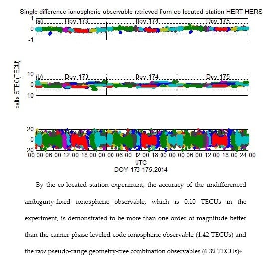
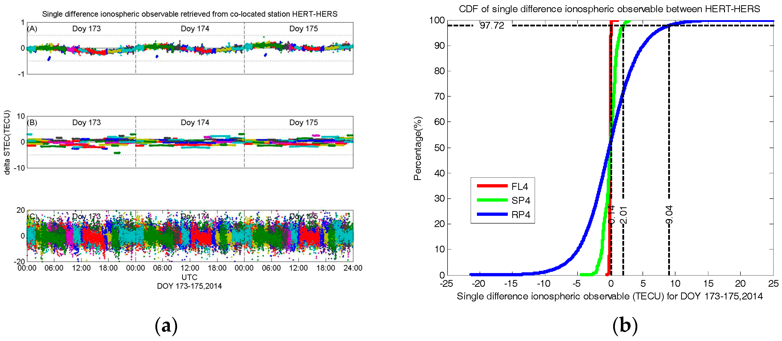
3.2. Accuracy Assessment of the Ionospheric Observable

The following analysis is illustrated using one co-located station pair, HERT-HERS during DOY 173–175, 2014. The results are representative of all of the other experimental pairs, summarized in what follows.

Figure 1a shows the single difference FL4, SP4 and raw pseudo-range geometry-free combination observables (designated as “RP4” hereafter) between co-located station HERT-HERS from DOY 173 to 175, 2014. Generally, a good agreement of the data from different satellites, represented with different colors, can be seen.

From the top panel of Figure 1a, a peak-to-peak value of the single difference FL4 observable for HERT-HERS configuration, ranging of about 0.28 TECU, is shown. According to Equation (8), this single difference is dominated by the observation error, including the instabilities of the receiver DCB, as well as the combination of the noise and multipath effects. Assuming the variations of both receivers are uncorrelated, the observation error of about $\frac{0.28/\sqrt{2}}{2}\approx 0.10$ TECUs can be found in the HERT-HERS configuration (the $\sqrt{2}$ stems from the assumption that the error of a single-difference observation is roughly $\sqrt{2}$ greater than the error of un-difference ones; the denominator 2 indicates a 95% significance is used to evaluate the observational error).

The middle panel of Figure 1a shows the single difference SP4 observable using a y-scale ten times greater than in the top panel. It is apparent that the peak-to-peak value of the middle panel is larger than that of the top panel and the middle panel shows an arc-to-arc dependence. Numerically, a peak-to-peak value of almost 4.02 TECUs is observed, indicating the observation error of the SP4 observable is about $\frac{4.02/\sqrt{2}}{2}\approx 1.42$ TECUs, more than one order of magnitude larger than the FL4 observable.

Complementarily, an analogous result can be achieved from the bottom panel of Figure 1a, where the single difference STEC from the RP4 observable is presented. The single-difference STEC from the RP4 observable is noisier, with a peak-to-peak value of almost 18.08 TECUs, indicating the observation error of the RP4 observable is about $\frac{18.08/\sqrt{2}}{2}\approx 6.39$ TECUs. Thus, the RP4 observable has the lowest accuracy, which is one to two orders of magnitude worse than the FL4 observable.

To quantify the reduction of the observation error, the Cumulative Distribution Function (CDF) of single difference FL4, SP4 and RP4 ionospheric observable for HERS-HERT station pair (after removing the mean value, see

Table 5. Summary results of the mean, standard deviation and observation error of the single difference ionospheric observable between the co-located receivers for all the satellites arcs for DOY 173 to 175, 2014.

Baseline	Single Difference Ionospheric Observable (TECU)
Station Pairs	FL4			SP4			RP4
Name	Mean	Stdev	Error	Mean	Stdev	Error	Mean	Stdev	Error
HERT-HERS	−5.22	0.14	0.10	0.07	2.01	1.42	0.07	9.04	6.39
DGAR-DGAV	23.69	0.32	0.23	27.20	2.49	1.76	27.20	18.41	13.02
THTI-FAA1	73.30	0.47	0.33	77.90	5.33	3.77	77.84	11.81	8.35
SUTH-SUTM	34.66	0.17	0.12	34.18	4.00	2.83	34.19	22.99	16.26
SUTH-SUTV	5.36	0.17	0.12	4.02	1.78	1.26	4.01	8.75	6.19
SUTM-SUTV	29.30	0.27	0.19	30.17	4.07	2.88	30.17	21.18	14.98
CONZ-CONT	−42.12	0.50	0.35	−32.88	1.71	1.21	−32.90	9.72	6.87
OUS2-OUSD	65.17	0.18	0.13	61.51	4.21	2.98	61.49	22.13	15.65

) are shown in Figure 1b. The plot intersects with the horizontal dash line marks the 95% significance of each single difference ionospheric observable.

According to Figure 1b, we can see that the standard deviation of the single difference FL4 observable is 0.14 TECUs while that of the single difference SP4 and RP4 observable are 2.01 and 9.04 TECUs, respectively.

The above results are based on the HERT-HERS configuration. Furthermore, Table 5 presents the Mean, Stdev and Error of the single difference FL4, SP4 and RP4 observable for the eight pairs of co-located stations according to their corresponding CDF information.

From Table 5, we can conclude that the FL4 observable is more accurate, followed in order by the SP4 and RP4 observables. Numerically, the observation errors affecting the FL4 observable range from 0.10 to 0.35 TECUs whereas errors for the SP4 (RP4) observable are from 1.21 to 3.77 TECUs (6.19 to 16.26 TECUs), indicating that the FL4 observable is over one order of magnitude more accurate than the SP4 and RP4 observables.

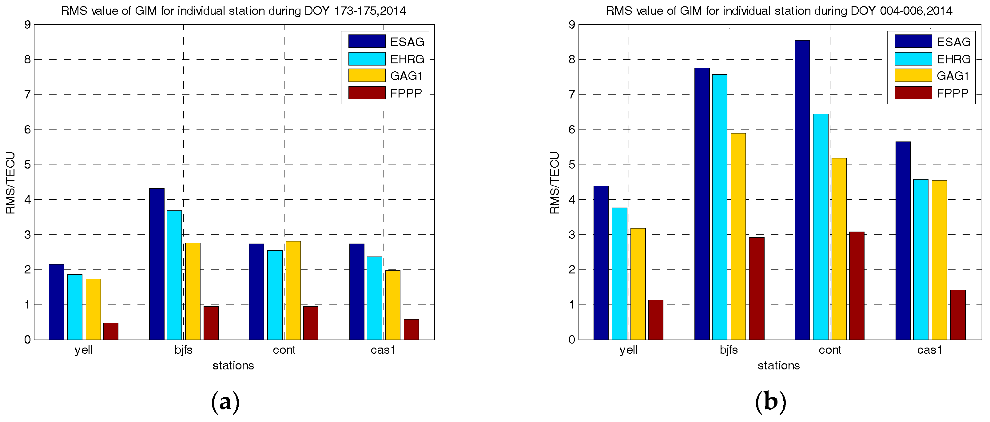
3.3. Accuracy Assessment of the Global Ionosphere Model

Table 6. The RMS of individual station for Case 1 (TECU).

Stations	UCOR	KLOB	ESAG	EHRG	GAG1	FPPP
yell	25.21	6.67	2.15	1.87	1.73	0.46
bjfs	34.42	9.73	4.29	3.68	2.74	0.95
cont	14.54	7.72	2.73	2.55	2.80	0.95
cas1	9.30	13.80	2.72	2.35	1.96	0.56

and

Table 7. The RMS of individual station for Case 2 (TECU).

Stations	UCOR	KLOB	ESAG	EHRG	GAG1	FPPP
yell	23.73	23.87	4.39	3.75	3.18	1.12
bjfs	34.09	22.34	7.76	7.57	5.88	2.91
cont	61.43	16.57	8.55	6.43	5.18	3.06
cas1	40.68	22.21	5.65	4.56	4.55	1.40

present the RMS value (see Equation (10)) of the ionosphere model for Case 1 and Case 2, respectively. For a better comparison, we also present the results of the uncorrected (representing the amount of the ionosphere delay, UCOR) and Klobuchar (KLOB) model. The results are also plotted in Figure 2 to gain a better visibility.

From Table 6 and Table 7, we can find that (1) in both cases, the FPPP model has the smallest RMS value, followed in order by GAG1, EHRG and ESAG; (2) when solar activity is high, the accuracy of the ionosphere model decreases; (3) the accuracy of the ionosphere model improves when the interval of the model gets small, as in the case of ESAG and EHRG; (4) the accuracy comparison of EHRG and GAG1 shows the advantage of the FL4 observable with regard to the SP4 observable; (5) FPPP, a two-layer ionosphere model with 15 min interval, shows great improvement, comparing with the GAG1 model.

Table 8. The overall RMS based on all the stations for Case 1 and Case 2 (TECU).

Cases	UCOR	KLOB	ESAG	EHRG	GAG1	FPPP
Case 1	20.87	9.48	2.97	2.61	2.31	0.73
Case 2	39.98	21.25	6.59	5.58	4.69	2.12

summarizes the RMS value based on all the four stations for Case 1 and Case 2. As can be seen, the accuracy of the FPPP model is better than 1 TECU when solar activity is low. On the other hand, the RMS of the FPPP model is about 2 TECU when solar activity is high. An interesting finding is that the accuracy of the GAG1 are 2.31 TECUs for Case 1 while the accuracy of the input of the GAG1 model, i.e., the FL4 observable, is below 0.35 TECUs. Therefore, the difference between the accuracy of the GAG1 and FL4 observable may contribute to the model error of GAG1 when using the SH model to represent structure of the ionosphere. Note that these accuracies may be a bit optimistic because the selected four stations are almost all used to generate the four GIM (except station BJFS in model EHRG). However, it is not critical that a particular station is (or not) used by a GIM, as once the GIMs are smoothed the accuracy is maintained up to few hundreds of kilometers from the stations used to derive the ionospheric model [6,30]. This is confirmed by comparing the results in Table 6 and Table 7 for station BJFS and model EHRG and ESAG.

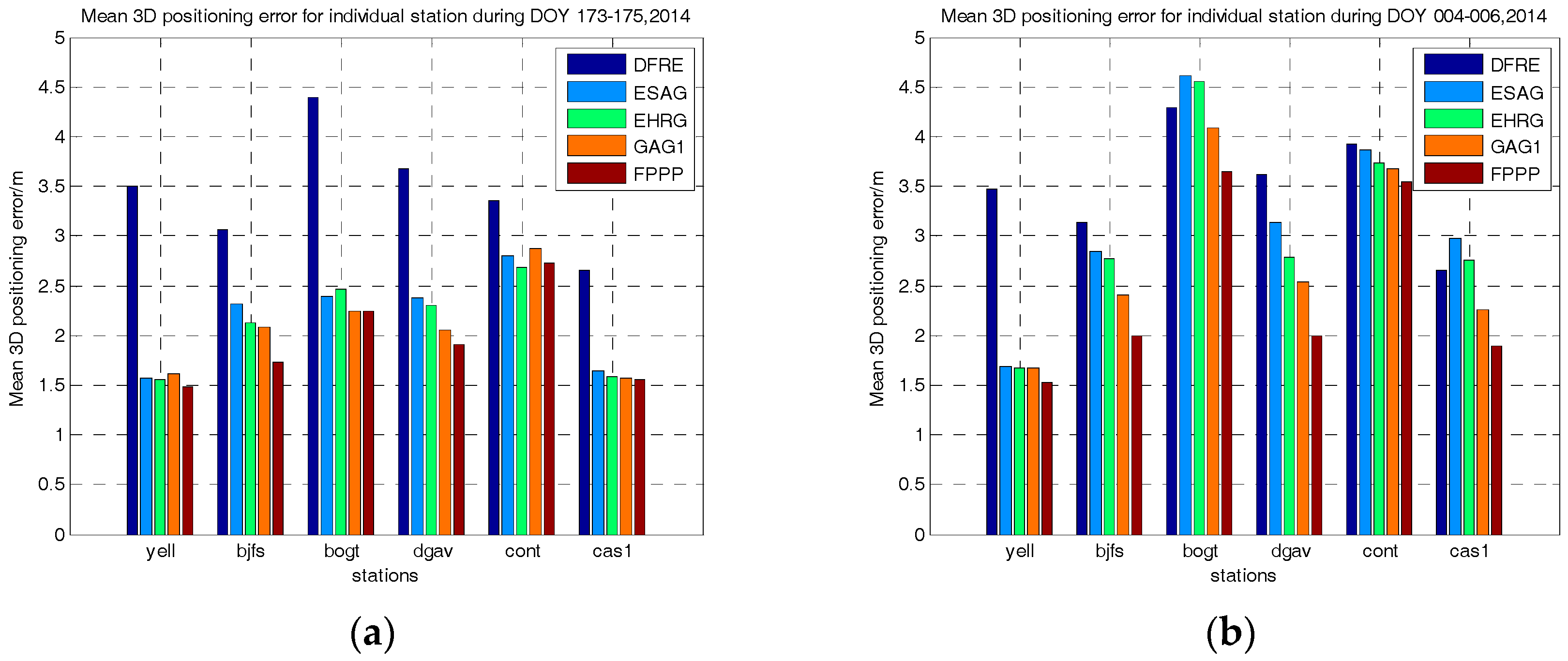
3.4. Single-Frequency Standard Point Positioning Experiment Test

In order to test and compare the different methods for the mitigation of the ionospheric error, single-frequency standard point positioning experiments are employed during the above two cases (Case 1 and Case 2). The following seven strategies are employed as follows:

• UCOR. Single-frequency observable (C1), no ionospheric model, and DCB from Navigation Message.
• KLOB. Single-frequency observable (C1), Klobuchar model, and DCB from Navigation Message.
• DFRE. Dual-frequency observable (P3).
• ESAG/EHRG/GAG1/FPPP. Single-frequency observable (C1), corresponding ionospheric model, and DCB from Navigation Message

The mean 3D positioning error of the individual stations are presented in Figure 3, standing for Case 1 and Case 2, respectively.

From Figure 3, we can conclude that (1) during the high solar activity, the quality of the single-frequency point positioning degrades when using the GIMs to mitigate the effects of the ionosphere. (2) when solar activity is low, the positioning accuracy of using GIMs is better than the dual-frequency ionosphere-free combination (DFRE); (3) In both cases, FPPP performs the best among the other GIMs, followed in increasing order of error by GAG1, EHRG and ESAG. In detail, with regard to the EHRG model, the improvement of the positioning accuracy using the FPPP can reach to as much as 32% and 38% for the station BJFS in Case 1 and Case 2.

4. Discussion

In this contribution, the accuracy of the undifferenced ambiguity-fixed ionospheric observable and carrier-phase leveled-code ionospheric observable are assessed firstly by the co-located experiment. The assessment proves that the accuracy of the FL4 observable is more than one order of magnitude better than the SP4 observable. Taking the FL4 observable as reference, the accuracy of the ESAG/EHRG/GAG1/FPPP global ionosphere models are assessed then. The comparison between EHRG and GAG1 shows that the impact of the ionospheric observable on the ionosphere model because EHRG and GAG1 both use the SH model with an interval of 1 h while the input of EHRG is SP4 observable and that of GAG1 is FL4 observable. Results show that the use of FL4 observable as the input of GIM improves the accuracy of the ionosphere model. The reason is discussed below. In addition, the comparison of the GAG1 and FPPP presents the impact of the mathematical model on the ionosphere model because GAG1 and FPPP both use the FL4 observable as the input of the ionosphere model while the mathematical model of GAG1 is a single-layer-based SH model and that of FPPP is a two-layer grid model. Therefore, the use of a two-layer model improves the accuracy of the ionosphere model further.

The single-frequency point positioning experiment has been adopted to test the above different ionosphere models to see their mitigation effects on the ionosphere delay. We show that the positioning errors reflect the accuracy of the different ionosphere models. By comparing Figure 2a,b, we can see that the positioning accuracy of the FPPP during the two cases is the best, followed by the GAG1, EHRG and ESGA. This phenomenon agrees with the conclusion from Table 8 that the RMS value of FPPP is the lowest (0.73 and 2.12 TECUs) in the two cases. Besides, the positioning accuracy degrades using GIMs during the high solar activity period, which can also be reflected from Table 8, that the RMS value of the GIMs becomes larger (2.12 to 6.59 TECUs) in Case 2 (high solar activity) than that (0.73 to 2.97 TECUs) in Case 1. As is known that during the high solar activity period, the structure of ionosphere TEC is more complex than that during the low solar activity period.

Another important phenomenon is that the accuracy of the GAG1 model seems to be only a little better than the EHRG, as shown in Table 8 and reflected from Figure 3. However, the FL4 observable used in GAG1 has been demonstrated to be over one order of magnitude better than the SP4 observable used in EHRG. This may be explained by the mathematical model error of SH. As introduced, the accuracy of the GIM depends on both the ionospheric observable and mathematical model. From the accuracy of the GAG1 model, we can deduce that the accuracy of the SH mathematical model is about 2–5 TECUs in our experiment. Thus, the accuracy of the FL4 observable (0.10 to 0.35 TECUs) used in the GAG1 model cannot be revealed due to magnitude of the mathematical error (2–5 TECUs). Again, the comparison of GAG1 and FPPP depicts the importance of the mathematical model. As presented in Table 8, the accuracy of FPPP is over a factor of 2 better than the GAG1. According to Table 2, this improvement can be attributed to the two-layer model with a 15-min interval. Other factors, such as the amount of the stations used to establish the GIM and the use of multi-GNSS data are deserved to do more research.

5. Conclusions

By the co-located station experiment, the accuracy of the undifferenced ambiguity-fixed ionospheric observable, which ranges from 0.10 to 0.35 TECUs, is demonstrated to be more than one order of magnitude better than the carrier-phase leveled-code ionospheric observable (1.21 to 3.77 TECUs). In addition, to model the global ionosphere structure, a two-layer ionosphere model has been used to generate the GIM.

Taking the undifferenced ambiguity-fixed ionospheric observable as reference, the accuracies of four different GIMs, namely ESAG, EHRG, GAG1 and FPPP, are assessed. Among the four different GIMs, EHRG and GAG1 differs in the ionospheric observable while both use the SH mathematical model. On the other hand, GAG1 and FPPP differ in the mathematical model while both use the FL4 observable. Results demonstrate that the accuracy of FL4-based GAG1 is only a little better than SP4-based EHRG due to the accuracy loss of the SH mathematical model. Additionally, the accuracy of the two-layer-based FPPP, which is two times better than the SH-based GAG1, demonstrates the significance of the mathematical model. Finally, the single-frequency point positioning experiment is adopted to test the GIMs. Positioning results show that, with regard to the EHRG, the improvement of the positioning accuracy using the FPPP can reach to as much as 32% in the low solar activity period and 38% in the high solar activity period in the research.

Therefore, both the ionospheric observable and the mathematical model should be taken into consideration during the generation of the GIM. Particularly, the undifferenced ambiguity-fixed ionospheric observable and two-layer ionosphere models are recommended.

References

1. Hargreaves, J. Principles of Ionosphere; Cambridge University Press: Cambridge, UK, 1992. [Google Scholar]
2. Krypiak-Gregorczyk, A.; Wielgosz, P.; Borkowski, A. Ionosphere Model for European Region Based on Multi-GNSS Data and TPS Interpolation. Remote Sens. 2017, 9, 1221. [Google Scholar] [CrossRef]
3. Rovira-Garcia, A.; Juan, J.M.; Sanz, J.; González-Casado, G.; Bertran, E. Fast Precise Point Positioning: A System to Provide Corrections for Single and Multi-frequency Navigation. Navigation 2016, 63, 231–247. [Google Scholar] [CrossRef] [Green Version]
4. Li, X.; Zhang, X.; Ge, M. Regional reference network augmented precise point positioning for instantaneous ambiguity resolution. J. Geodesy 2011, 85, 151–158. [Google Scholar] [CrossRef]
5. Li, X. Improving real-time PPP ambiguity resolution with ionospheric characteristic consideration. In Proceedings of the ION GNSS-12, Institute of Navigation, Nashville, TN, USA, 17–21 September 2012. [Google Scholar]
6. Geng, J.; Meng, X.; Dodson, A.H.; Ge, M.; Teferle, F.N. Rapid re-convergences to ambiguity-fixed solutions in precise point positioning. J. Geodesy 2010, 84, 705–714. [Google Scholar] [CrossRef]
7. Geng, J.; Bock, Y. GLONASS fractional-cycle bias estimation across inhomogeneous receivers for PPP ambiguity resolution. J. Geodesy 2016, 90, 379–396. [Google Scholar] [CrossRef]
8. Geng, J.; Shi, C. Rapid initialization of real-time PPP by resolving undifferenced GPS and GLONASS ambiguities simultaneously. J. Geodesy 2017, 91, 361–374. [Google Scholar] [CrossRef]
9. Kashani, I.; Wielgosz, P.; Grejner-Brzezinska, D.A. The impact of the ionospheric correction latency on long baseline instantaneous kinematic GPS positioning. Surv. Rev. 2007, 39, 238–251. [Google Scholar] [CrossRef]
10. Mohino, E.; Gende, M.; Brunini, C. Improving long baseline (100–300 km) differential GPS positioning applying ionospheric corrections derived from multiple reference stations. J. Surv. Eng. 2007, 133, 1–5. [Google Scholar] [CrossRef]
11. Ren, X.; Zhang, X.; Xie, W.; Zhang, K.; Yuan, Y.; Li, X. Global ionospheric modelling using multi-GNSS: BeiDou, Galileo, GLONASS and GPS. Sci. Rep. 2016, 6, 33499. [Google Scholar] [CrossRef] [PubMed]
12. Jin, S.; Occhipinti, G.; Jin, R. GNSS ionospheric seismology: Recent observation evidences and characteristics. Earth-Sci. Rev. 2015, 147, 54–64. [Google Scholar] [CrossRef]
13. Komjathy, A.; Sparks, L.; Wilson, B.D.; Mannucci, A.J. Automated daily processing of more than 1000 ground-based GPS receivers for studying intense ionospheric storms. Radio Sci. 2005, 40. [Google Scholar] [CrossRef]
14. Van Dierendonck, A.J.; Klobuchar, J.; Hua, Q. Ionospheric scintillation monitoring using commercial single frequency C/A code receivers. In Proceedings of the 6th International Technical Meeting of the Satellite Division of The Institute of Navigation (ION GPS 1993), Salt Lake City, UT, USA, 22–24 September 1993; Volume 93, pp. 1333–1342. [Google Scholar]
15. Jakowski, N.; Heise, S.; Wehrenpfennig, A.; Schlüter, S.; Reimer, R. GPS/GLONASS-based TEC measurements as a contributor for space weather forecast. J. Atmos. Sol. Terr. Phys. 2002, 64, 729–735. [Google Scholar] [CrossRef]
16. Liu, J.Y.; Chen, Y.I.; Chen, C.H.; Liu, C.Y.; Chen, C.Y.; Nishihashi, M.; Li, J.Z.; Xia, Y.Q.; Oyama, K.I.; Hattori, K.; et al. Seismoionospheric GPS total electron content anomalies observed before the 12 May 2008 Mw7. 9 Wenchuan earthquake. J. Geophys. Res. Space Phys. 2009, 114. [Google Scholar] [CrossRef]
17. Savastano, G.; Komjathy, A.; Verkhoglyadova, O.; Mazzoni, A.; Crespi, M.; Wei, Y.; Mannucci, A.J. Real-Time Detection of Tsunami Ionospheric Disturbances with a Stand-Alone GNSS Receiver: A Preliminary Feasibility Demonstration. Sci. Rep. 2017, 7. [Google Scholar] [CrossRef] [PubMed]
18. Zhang, B.; Teunissen, P.J.; Yuan, Y. On the short-term temporal variations of GNSS receiver differential phase biases. J. Geodesy 2017, 91, 563–572. [Google Scholar] [CrossRef]
19. Wilson, B.D.; Mannucci, A.J. Instrumental biases in ionospheric measurements derived from GPS data. In Proceedings of the 6th International Technical Meeting of the Satellite Division of The Institute of Navigation (ION GPS 1993), Salt Lake City, UT, USA, 22–24 September 1993; pp. 1343–1351. [Google Scholar]
20. Manucci, A.J.; Iijima, B.A.; Lindqwister, U.J.; Pi, X.; Sparks, L.; Wilson, B.D. GPS and ionosphere. In URSI Reviews of Radio Science, 1996–1999; Stone, W.R., Ed.; Jet Propulsion Laboratory: Pasadena, CA, USA, 1999. [Google Scholar]
21. Schaer, S. Mapping and Predicting the Earth’s Ionosphere Using the Global Positioning System. Ph.D. Thesis, Astronomical Institute, University of Berne, Bern, Switzerland, 1999. [Google Scholar]
22. Manucci, A.J.; Wilson, B.D.; Yuan, D.N.; Ho, C.H.; Lindqwister, U.J.; Runge, T.F. A global mapping technique for GPS-derived ionospheric total electron content measurements. Radio Sci. 1998, 33, 565–582. [Google Scholar] [CrossRef]
23. Hernández-Pajares, M.; Roma, D.D.; Krankowski, A.; Ghoddousi, F.R.; Yuan, Y.; Li, Z.; Zhang, H.; Shi, C.; Feltens, J.; Komjathy, A.; et al. Comparing performances of seven different global VTEC ionospheric models in the IGS context. In Proceedings of the IGS Workshop, Sydney, Australia, 8–12 February 2016; pp. 1–31. [Google Scholar]
24. Ciraolo, L.; Azpilicueta, F.; Brunini, C.; Meza, A.; Radicella, S. Calibration errors on experimental slant total electron content (TEC) determined with GPS. J. Geodesy 2007, 81, 111–120. [Google Scholar] [CrossRef]
25. Blewitt, G. Carrier phase ambiguity resolution for the global positioning system applied to geodetic baselines up to 2000 km. J. Geophys. Res. 1989, 94, 10187–10203. [Google Scholar] [CrossRef]
26. Zumberge, J.F.; Heflin, M.B.; Jefferson, D.C.; Watkins, M.M.; Webb, F.H. Precise point positioning for the efficient and robust analysis of GPS data from large networks. J. Geophys. Res. Solid Earth 1997, B3, 5005–5017. [Google Scholar] [CrossRef]
27. Banville, S.; Zhang, W.; Ghoddousi-Fard, R.; Langley, R.B. Ionospheric Monitoring Using Integer-Levelled Observations. In Proceedings of the 25th International Technical Meeting of the Satellite Division of the Institute of Navigation (ION GNSS 2012), Nashville, TN, USA, 17–21 September 2012; pp. 2692–2701. [Google Scholar]
28. Zhang, B.; Ou, J.; Yuan, Y.; Li, Z. Extraction of line-of-sight ionospheric observables from GPS data using precise point positioning. Sci. China Earth Sci. 2012, 55, 1919–1928. [Google Scholar] [CrossRef]
29. Zhang, B. Three methods to retrieve slant total electron content measurements from ground-based GPS receivers and performance assessment. Radio Sci. 2016, 51, 972–988. [Google Scholar] [CrossRef]
30. Rovira-Garcia, A.; Juan, J.M.; Sanz, J.; González-Casado, G. A World-Wide Ionospheric Model for Fast Precise Point Positioning. IEEE Trans. Geosci. Remote Sens. 2015, 53, 4596–4604. [Google Scholar] [CrossRef]
31. Rovira-Garcia, A.; Juan, J.M.; Sanz, J.; González-Casado, G.; Ibáñez-Segura, D. Accuracy of ionospheric models used in GNSS and SBAS: Methodology and analysis. J. Geodesy 2016, 90, 229–240. [Google Scholar] [CrossRef]
32. Bossler, J.D.; Goad, C.C.; Bender, P.L. Using the global positioning system (gps) for geodetic positioning. Bull. Géodésique 1980, 54, 553–563. [Google Scholar] [CrossRef]
33. Braasch, M. Multi-path effects. In Global Positioning System: Theory and Applications, Volume 1 (Progress in Astronautics and Aeronautics); Parkinson, B.W., Spilker, J.J., Eds.; American Institute of Aeronautics and Astronautics: Reston, VA, USA, 1996; pp. 547–568. [Google Scholar]
34. Dow, J.M.; Neilan, R.; Rizos, C. The international GNSS service in a changing landscape of global navigation satellite systems. J. Geodesy 2009, 83, 191–198. [Google Scholar] [CrossRef]
35. Laurichesse, D.; Mercier, F. Integer Ambiguity resolution on undifferenced GPS phase measurements and its application to PPP. In Proceedings of the 20th International Technical Meeting of the Satellite Division, Institute of Navigation, Fort Worth, TX, USA, 25–28 September 2007; pp. 839–848. [Google Scholar]
36. Collins, P.; Lahaye, F.; Heroux, P.; Bisnath, S. Precise point positioning with ambiguity resolution using the decoupled clock model. In Proceedings of the ION GNSS 2008, Savannah, GA, USA, 25–29 September 2017; pp. 1315–1322. [Google Scholar]
37. Ge, M.; Gendt, G.; Dick, G.; Zhang, F.P. Improving carrier-phase ambiguity resolution in global GPS network solutions. J. Geodesy 2005, 79, 103–110. [Google Scholar] [CrossRef]
38. Hernández-Pajares, M.; Juan, J.; Sanz, J.; Orus, R.; Garcia-Rigo, A.; Feltens, J.; Komjathy, A.; Schaer, S.; Krankowski, A. The IGS VTEC maps: A reliable source of ionospheric information since 1998. J. Geodesy 2009, 83, 263–275. [Google Scholar] [CrossRef]
39. Sanz, J.; Juan, J.; Hernández-Pajares, M. GNSS Data Processing, Vol. I: Fundamentals and Algorithms; ESTEC TM-23/1; ESA Communications: Noordwijk, The Netherlands, 2013. [Google Scholar]
40. Juan, J.M.; Rius, A.; Hernández-Pajares, M.; Sanz, J. A two-layer model of the ionosphere using Global Positioning System data. Geophys. Res. Lett. 1997, 24, 393–396. [Google Scholar] [CrossRef]
41. Brunini, C.; Azpilicueta, F.J. Accuracy assessment of the GPS-based slant total electron content. J. Geodesy 2009, 83, 773–785. [Google Scholar] [CrossRef]
42. Øvstedal, O. Absolute positioning with single-frequency GPS receivers. GPS Solut. 2002, 5, 33–44. [Google Scholar] [CrossRef]
43. Space Physics Interactive Data Resource (SPIDR). Available online: http://spidr.ngdc.noaa.gov/spidr/dataset.do (accessed on 1 November 2017).
44. Covington, A.E. Solar Radio Emission at 10.7 cm, 1947–1968. J. R. Astron. Soc. Can. 1969, 63, 125–132. [Google Scholar]
45. Fagundes, P.R.; Pillat, V.G.; Bolzan, M.J.A.; Sahai, Y.; Becker-Guedes, F.; Abalde, J.R.; Aranha, S.L. Observations of F layer electron density profiles modulated by planetary wave type oscillations in the equatorial ionospheric anomaly region. J. Geophys. Res. 2005, 110. [Google Scholar] [CrossRef]
46. Hatch, R. The synergism of GPS code and carrier measurements. In Proceedings of the Third International Symposium on Satellite Doppler Positioning at Physical Sciences Laboratory of New Mexico State University, Las Cruces, NM, USA, 8–12 February 1982; Volume 2, pp. 1213–1231. [Google Scholar]
47. Melbourne, W.G. The case for ranging in GPS-based geodetic systems. In Proceedings of the First International Symposium on Precise Positioning with the Global Positioning System, Rockville, MD, USA, 15–19 April 1985; p. 1519. [Google Scholar]
48. Wubbena, G. Software developments for geodetic positioning with GPS using TI-4100 code and carrier measurements. In Proceedings of the First International Symposium on Precise Positioning with the Global Positioning System, Rockville, MD, USA, 15–19 April 1985; p. 19. [Google Scholar]
Figure 1. Single difference ionospheric observable retrieved from co-located station HERT-HERS from DOY 173 to 175, 2014, using (A) FL4 (B) SP4 (C) RP4 observable (a) and the cumulative distribution function (CDF) of single difference FL4, SP4 and RP4 observable (after removing the mean value, see Table 5) from the co-located station HERT-HERS (b).
Remotesensing 10 00169 g001
Figure 2. The RMS of individual station for Case 1 (a) and Case 2 (b).
Remotesensing 10 00169 g002
Figure 3. Mean 3D positioning error of individual station for Case 1 (a) and Case 2 (b).
Remotesensing 10 00169 g003