The Role of NWP Filter for the Satellite Based Detection of Cumulonimbus Clouds


German Weather Service, Frankfurter Str 135, 63067 Offenbach, Germany
*
Author to whom correspondence should be addressed.
Remote Sens. 2018, 10(3), 386; https://doi.org/10.3390/rs10030386
Submission received: 28 November 2017
/
Revised: 22 February 2018
/
Accepted: 26 February 2018
/
Published: 2 March 2018
(This article belongs to the Special Issue Remote Sensing Methods and Applications for Traffic Meteorology)
Abstract
:This study is motivated by the great importance of Cbs for aviation safety. The study investigates the role of Numerical Weather Prediction (NWP) filtering for the remote sensing of Cumulonimbus Clouds (Cbs) by implementation of about 30 different experiments, covering Central Europe. These experiments compile different stability filter settings as well as the use of different channels for the InfraRed (IR) brightness temperatures (BT). As stability filters, parameters from Numerical Weather Prediction (NWP) are used. The application of the stability filters restricts the detection of Cbs to regions with a labile atmosphere. Various NWP filter settings are investigated in the experiments. The brightness temperature information results from the infrared (IR) Spinning Enhanced Visible and InfraRed Image (SEVIRI) instrument on-board of the Meteosat Second Generation satellite and enables the detection of very cold and high clouds close to the tropopause. Various satellite channels and BT thresholds are applied in the different experiments. The satellite only approaches (no NWP filtering) result in the detection of Cbs with a relative high probability of detection, but unfortunately combined with a large False Alarm Rate (FAR), leading to a Critical Success Index (CSI) below 60% for the investigated summer period in 2016. The false alarms result from other types of very cold and high clouds. It is shown that the false alarms can be significantly decreased by application of an appropriate NWP stability filter, leading to the increase of CSI to about 70% for 2016. CSI is increased from about 70 to about 75% by application of NWP filtering for the other investigated summer period in 2017. A brief review and reflection of the literature clarify that the function of the NWP filter can not be replaced by MSG IR spectroscopy. Thus, NWP filtering is strongly recommended to increase the quality of satellite based Cb detection. Further, it has been shown that the well established convective available potential energy (CAPE) and the convection index (KO) work well as a stability filter.
1. Introduction
Cumulonimbus clouds (Cbs) originate from rapid vertical updraft of humid and warm air enforced by constraint forces caused e.g., by mountains, heating or cold fronts. The fast cooling of the air with rising altitude leads to optically thick and very cold clouds, referred to as cumulonimbus clouds (Cbs), which are usually accompanied by lightning, heavy precipitation, hail, and turbulence. Early and reliable prediction of Cb clouds is therefore of great importance for weather forecasts and warnings, in particular for aviation, as Cb clouds (thunderstorms) constitute one of the most important natural risks for aircraft accidents. An accurate Cb detection and short term forecast enables cost-efficient planning and use of alternative routes, thus increasing flight safety.
Yet, the reliable simulation of convective cells and Cbs by means of numerical weather prediction is still a very difficult task. Thus, observational data plays a pivotal role for the accurate detection and short term forecast of Cbs. Over ocean and a vast number of countries, which are not well equipped with precipitation RADARs, satellites are in addition to global ground based lightning networks the only observational source for the detection of Cbs, e.g., [1]. As a result of the thermodynamics involved in the generation of Cbs they are optically thick and their tops are located close to the tropopause. Therefore, from a satellite perspective they are characterized by very cold brightness temperatures corresponding to high cloud top heights (CTH).
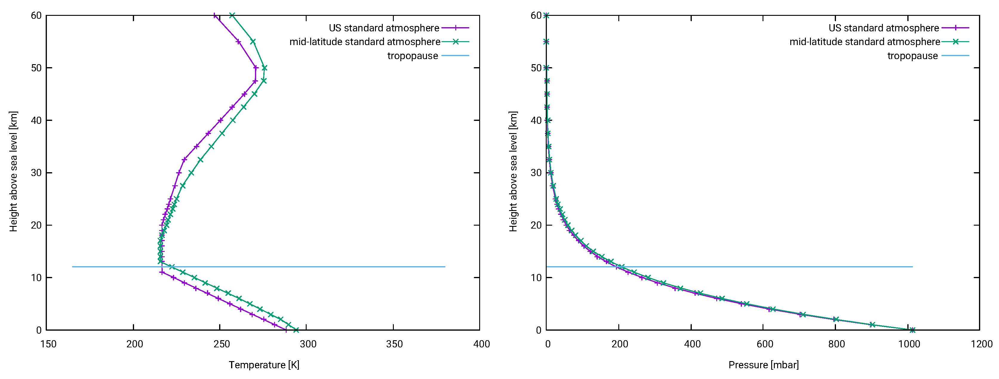
As a result, cloud top height is an option used as a straightforward method to provide information about the risk for cumulonimbus cloud occurrence as operated by, e.g., NCAR ([2] and references therein). The cloud top height can be derived from the brightness temperature (BT) in the atmospheric window channel (InfraRed 10.6), which corresponds in good approximation with the temperature of the cloud top for Cbs. A NWP based profile of the atmosphere can then be used to link the temperature to the height of the cloud top, see Figure 1 for an example of an atmospheric profile. A more detailed discussion of methods for the estimation of CTH are presented in [3].
Another simple, but widely used method is that applied in the Global Convective Diagnostics approach [2,4]. The method uses the brightness temperature difference between the 6.7 m the 11.6 m infrared satellite channel, the former is also referred to as water vapour channel, because of the strong water vapour absorption bands. If the BT difference exceeds 1 degree Kelvin (K) it is assumed that the observed cloud is a cumulonimbus cloud. The physical background of this approach has been already discussed in 1997 by Schmetz et al. [5]. They investigated the potential of satellite observation for the monitoring of deep convection and overshooting tops. They found that the brightness temperature of the water vapor channel (5.7–7.1 m) can be larger (warmer) than that of the IR window channel (10.5–12.5 m). They demonstrated by radiative transfer modeling (RTM) that the larger brightness temperatures (BT) in the WV channel are due to stratospheric (tropopause) water vapor, which absorbs radiation from the cold cloud and subsequently emits radiation at higher temperature (warmer), as the temperature increases in the stratosphere, see Figure 1. The effect is largest when the cloud top is at the tropopause temperature inversion. Optically thick high clouds cover the tropospheric water vapor and only the emission from the stratospheric water vapor contributes to the radiance observed by the satellite instrument. In contrast, for lower clouds the tropospheric water vapor above the clouds absorbs the radiation and the emitted radiation is colder than the absorbed. It is therefore obvious that the temperature difference increases with increasing cloud height.
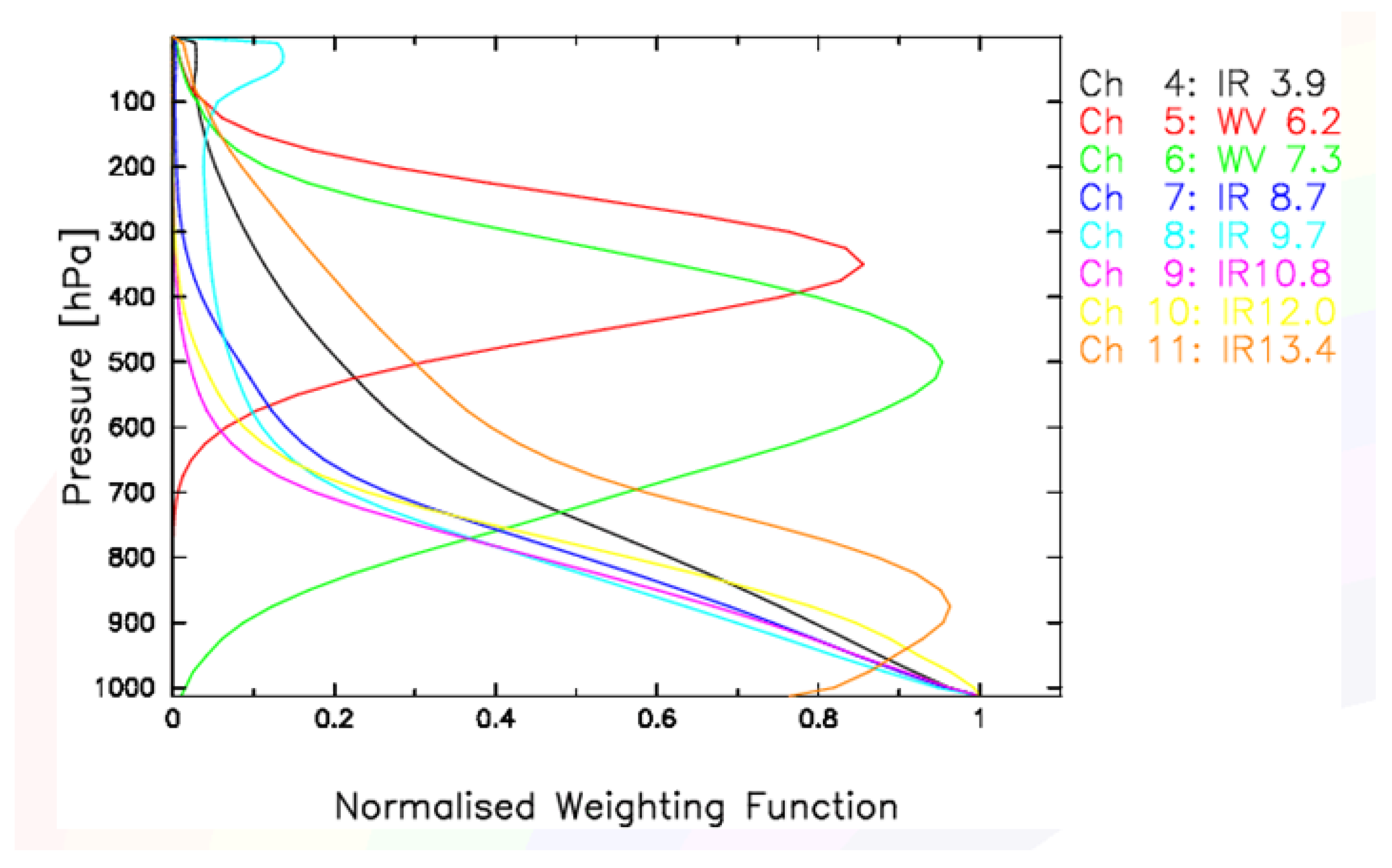
The effect discussed by [5] occurs also if the difference of the two water vapor channels are used. The use of this combination is possible since the launch of Meteosat Second Generation satellites, which has the Spinning Enhanced Visible and InfraRed Image (SEVIRI) instrument on-board. This instrument is equipped with additional channels in the Infrared (IR). The normalized weighting function of the SEVIRI IR channels is shown in Figure 2 for clear sky.
Note, that the water vapor channel at 6.2 m receives significant contributions from the stratosphere, which are larger than the equivalent contributions of the WV channel at 7.3 m. Thus, the mechanism discussed by Schmetz et al. [5] works also well for the difference of the water vapor channels.
A slightly different approach is used by the Nowcasting Satellite Application Facility NWC-SAF. This method is based upon an adaptive brightness temperature thresholds of infrared images [6]. Further, cloud classification methods have been developed which use texture information of the visible channels in addition to the brightness temperature thresholds to detect Cbs and other cloud types. The NRL Cloud Classification (CC) algorithm [7] is one example. It is used by the Oceanic Weather Product Development Team to assist in the accurate detection of deep convective clouds. Another example is the Berendes cloud mask [8]. However, in both methods visible channels are utilized and they are therefore not applicable during night. Thus, these approaches are not sufficient to provide a day and night service needed by aviation. Finally, there exists a commercially offered software package, which has been developed and validated by Zinner et al. [9] and references therein.
All these approaches use information from the IR region for the satellite based detection of Cbs. However, also other clouds are optically thick and cold (e.g., Nimbostratus and Stratocumulus II), which can lead to serious false alarms. As briefly discussed in [2] these false alarms might be reduced by the implementation of an stability filer from NWP.
To the knowledge of the authors, a NWP filter is either not applied in the above mentioned methods (e.g., [7,8,9] ) or an extensive analysis and discussion of NWP filtering based on extensive validation experiments have not been provided ([2,4,6]). Further, the role of NWP filtering is not reflected in relation to IR spectroscopy. Thus, the central novel aspect of this work is the extensive discussion and analysis of NWP filtering for the quality of satellite based Cb detection, including a reflection of SEVIRI IR spectroscopy as alternative.
2. Materials and Methods
The difference of the brightness temperature of the WV channels of the SEVIRI instrument on board of the Meteosat Second Generation satellite (MSG) is used as starting point of the study and in the majority of the experiments. This approach is based on the method discussed in [5] and more recently applied by e.g., [2,4]. However, in our method, the WV 7.3 channel is used instead of the atmospheric window channel for the calculation of the brightness temperature difference.
Further, in contrast to [2] a threshold of −1 K is applied in the first experiments. However, further experiments are performed with different thresholds. As the temperature signal of Cbs is not only apparent in the WV channels the performance of further channels combinations are investigated in the experiments as well.
The satellite brightness temperatures are derived from the level 1.5 rectified image data of digital counts by application of the Eumetsat calibration coefficients and conversation method. More detailed information on MSG and the SEVIRI instrument are given in [10].
For the stability filter the well established convective available potential energy (CAPE) is used [11]. CAPE is the amount of energy a parcel of air would have if lifted a certain distance vertically through the atmosphere. It is effectively the positive buoyancy of an air parcel.
As a supplementing filter to CAPE the Totals Total (TT) index has been used. It is defined as:
here T is the temperature, is the dew point temperature and the numbers provide the respective pressure level.
Further, the KO index defined in Equation (2) has been applied in further experiments;
here is the pseudo potential temperature in Kelvin for the different pressure levels 1000, 850, 700 and 500 hPa.
For CAPE and TT the forecast runs of the ECMWF operational model [12] at 0 h and 12 h has been used. This means that forecasts up to 9 h are applied. The stability parameter (KO, CAPE) results from the DWD numerical weather prediction model ICON [13] for the 2017 period. In contrast to ECMWF ICON forecast runs are applied every 3 h. Thus, the respective run 3 h prior relative to the satellite scanning time has been used.
As initial values 60 and 3 have been choose for CAPE and KO, respectively, based on visual inspection of several cases and on advice from the weather forecasters at DWD. However, these values are varied within different validation experiments and the respective results are shown in Section 3.
The application of the NWP stability filter aims to restrict the detection of Cbs to regions with a labile atmosphere. Various NWP filter settings are investigated in the experiments. The “stability” filters (CAPE and TT) for the first experiments (up to experiment 8) are taken from the comprehensive Earth-system model developed at ECMWF in cooperation with Meteo-France. A detailed documentation of the model can be found at the ECMWF web-page, see [14] and concerning the convection part see, [12]. In order to investigate the sensitivity of the NWP filtering on the chosen NWP model, stability filters from ICON [13] have been also taken into account within the experiments. Within this scope, also KO provided by ICON has been investigated, following the advice of the DWD weather forecasters.
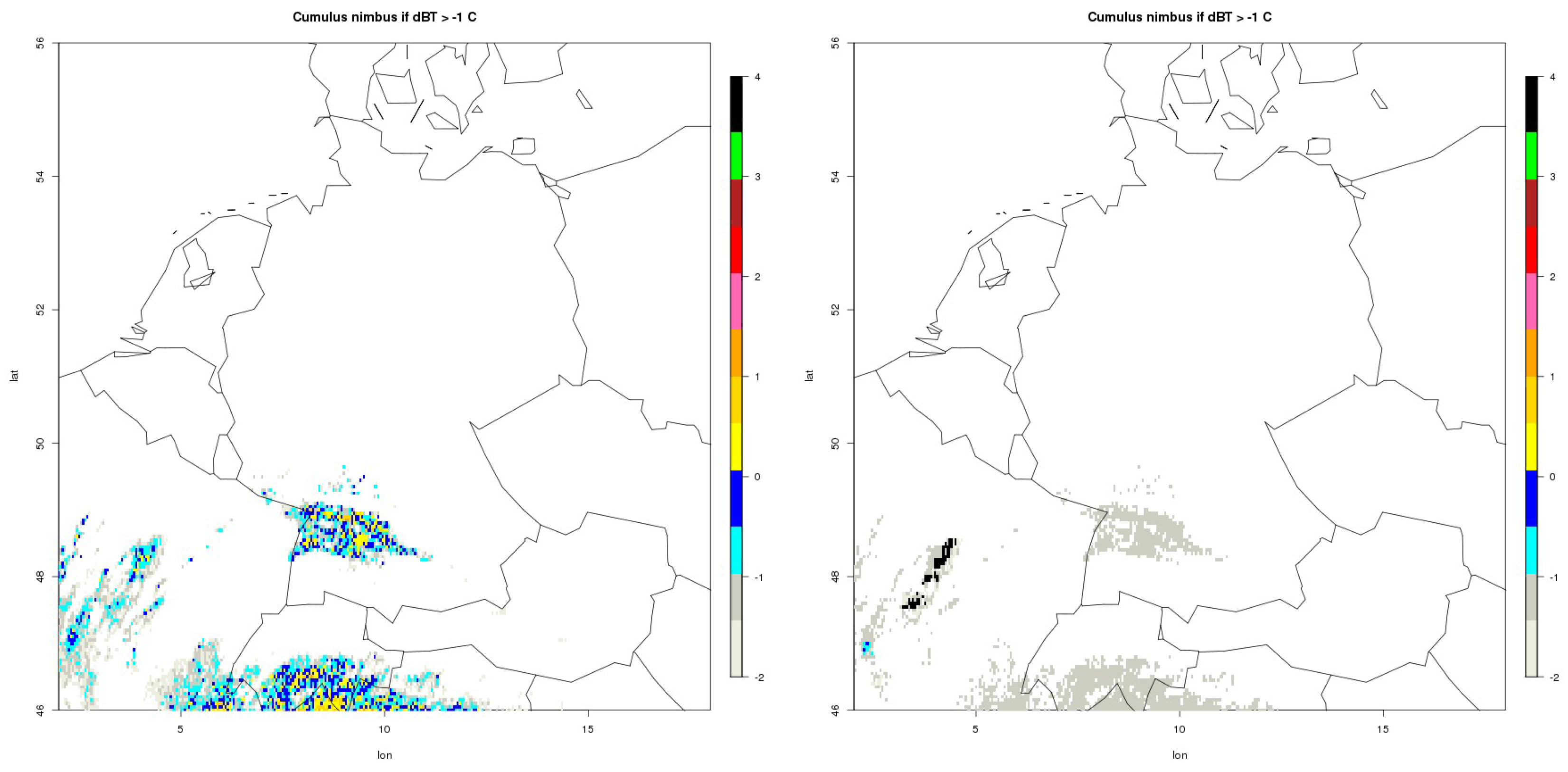
In the experiments with the NWP filters a Cb can only occur if the stability filters exceed the filter thresholds independent of the satellite signal. For the combination of CAPE and TOTALX it is an or operator conjunction, thus a Cb is assigned if one of the two filter thresholds is exceeded. For experiments without NWP filter Cb occurs if the BT difference is higher than the BT threshold defined for the respective experiment. With respect to the satellite part, various channels and BT thresholds are applied in the experiments. The respective settings are described in more detail in Table 1. Figure 3 illustrates the effect of the NWP filter on the satellite based Cb detection.
It is important to note that the aim of the stability filters is to avoid the false detection of Cbs by the satellite in stable and neutral atmospheres (e.g., cold fronts). Thus, the initial thresholds applied for the stability filters are not very strict.
Validation Scores and Settings
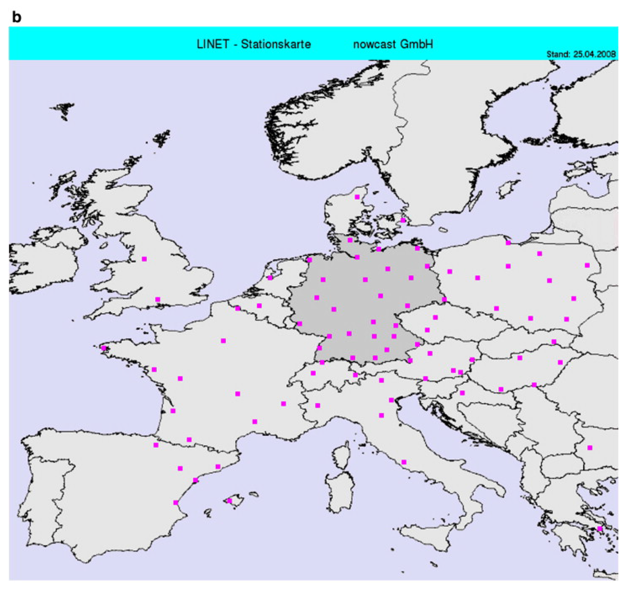
Lightning data from a low frequency (VLF/LF) lightning detection network (LINET), discussed in [15,16], are used for validation. The measurement network provides cloud-to-ground lightning strokes (CG) and inter-cloud lightning (IC). According to [15], the position accuracy reaches an average value of about 150 m, whereby false locations (‘outliers’) rarely occur. The study focuses on Central Europe where the LINET network density is highest, see Figure 4. The borders of the validation region are as follows: Latitude 45.5–56.5N and Longitude 2.0–18.0E. The skill scores Probability Of Detection (POD), False Alarm Rate (FAR), Critical Success Index (CSI) and the accuracy (ACC) are used to measure the performance of the different experiments. For completeness the quantities are defined below:
Hereby, CD stands for Correct Detection of a Cb, MD stands for Missed Detection of a Cb and FD stands for False Detection and CDN stands for Correct Detection of nil. The validation is performed on a pixel basis. This means that each pixel is assigned with either CD, FD, MD or CDN. CD, FD and MD are defined according to the criteria mentioned below.
Cloud lightning and cloud to ground lightning strokes are used for the validation if the amplitude is higher/lower than +/− 1 kA. A Cb is defined as correctly detected if lightning occurs within a 10 min time interval ending at the satellite scanning time of Central Europe and an search region (SR) of ±50 km. If there is no lightning, then a false alarm is counted. As a matter of fact, Cbs without strokes or artificial strokes are also possible, but this is not accounted for. This means that the performance of the method might be slightly better than expressed in the skill scores. Missed detection is counted if lightning occurs but there is no Cb detected by the satellite within the search region, whereby the four neighboring pixel to the stroke sites are counted.
The search region (SR) of ±50 km reflects the fact that larger Cbs are of most interest for aviation. Further, it accounts for the typical range of dislocations between lightning and the center of the Cb (approx. up to 15–20 km), as well as for the geolocation error of the satellite (approx 5 km), and for the safety distance defined for avoiding a Cb by flying around it. Please note , that this favors also large Cbs in the POD skill score. However, the selection of the search region is motivated by a “aviation forecaster’s” point of view, as large Cbs are of particular interest for aviation safety. It is important to note that the skill scores are dedicated for the inter-comparison of the performed experiments within the scope of this study. In general, a comparison of skill scores is only reasonable for identical periods, regions, reference data and validation settings (e.g., search region, pixel or object based validation, …). Thus, the skill scores presented in this manuscript are by no means dedicated as quality measures compared to other methods. In order to demonstrate the usability of the NWP filter for other applications, experiments with a smaller SR has been performed as well.
All experiments have been performed for for 6, 9, 12, 15, 18 UTC respectively. The majority of the experiments have been done for the period 10 May 2016 to 9 June 2016. However, the experiments dealing with KO and respective inter-comparison experiments, needed to evaluate the KO skill scores, have been performed for June 2017. This has been necessary as KO is not archived for the 2016 period. Both periods are characterized by frequent occurrence of Cbs for different weather situations, Cb size and structure. For the skill scores statistically significant populations has been examined. e.g., for the experiments without NWP filter 82,115 pixel are counted as hits, 44,733 as false alarms and 7464 as missed for the period in 2016 and for the 2017 period, 106,186 are counted as hits, 40,235 as false alarms and 4228 as missed.
Two experiments have been performed by using additionally the BT difference of the ozone channel (IR9.7) and the 8.7 channel (9.7–8.7). The IR9.7 channel is the ozone channel and has a clear sky emission peak in the stratosphere, see Figure 2. Thus, it can be assumed that clouds reaching the stratosphere (overshooting tops) show a pronounced signal if the ozone channel is used for the calculation of the BT difference as discussed e.g., by [17]. Overshooting tops are a specific feature of Cbs. Thus, the use of the ozone channel might be useful to omit the NWP filter at a certain BT difference (height), which has been investigated in experiment 5 and 6. However, the physical basis is the same as discussed in [5], but with the ozone emission interacting with the cloud emission instead of water vapour/cloud interaction.
3. Results
Table 1 as well as Figure 5 and Figure 6 show the skill scores of the experiments in detail. Table 1 shows the results for various satellite approaches, with fixed values for KO and CAPE (TT) switched on or off. Whereas, Figure 5 and Figure 6 show the effect of various CAPE and KO values for a fixed satellite approach (meaning a fixed BT difference threshold and satellite channel combination). In the following the main results of the experiments are summarized.
The results show that applying an NWP filtering can be used to optimize the relation of POD and FAR and thus, to improve the critical success index CSI. For the experiments with NWP filter, a relatively high POD in combination with a relatively low FAR can be gained, leading to significant better CSI than without NWP filtering.
POD is slightly higher without NWP filtering, but FAR is strongly affected towards higher values, leading to a significant decrease of CSI. However, compared to the experiments without NWP filtering higher POD can be achieved, accompanied by better CSI and FAR, by application of the NWP filter and lowering of the BT difference threshold. These results clearly demonstrate that the NWP filter does significantly increases the performance of the satellite based detection of Cbs.
The additional usage of the -channel experiment 5 and 6 does not lead to better skill scores compared to the reference (experiment 1). On the other hand, the one channel approach experiment 6 leads to similar skill scores compared to the reference (experiment 1). The physical basis of these results is further discussed in Section 4.
Finally, in experiment 9 and 10 CAPE from ICON has been used instead of CAPE from ECMWF. The results show that the skill scores are not significantly affected by the NWP source for CAPE. Thus, the NWP filtering is not sensitive to the NWP model in our experiments. Further, experiments for June 2017 have been performed with KO from ICON, as this stability filter has been recommended by the weather forecast department based on their daily practice. In order to evaluate the skill scores for KO intercomparison experiments for the same period have been performed with CAPE (as the skill scores are not independent on the chosen period). The investigated hours and the region are the same as for 2016. Thus the same number of samples have been used for the skill scores.
The results indicate that KO performs similarly to CAPE. In this experiment KO leads to higher POD, but due to also higher FAR, CSI is similar. The combination of KO and CAPE does not lead to better skill scores than KO alone.
The accuracy is close to 100% for all experiments and is therefore not an appropriate skill score for Cb detection, although, it is sometimes used as score for events with low probability of occurrence.
The experiments listed in the Table 1 show the effect of predefined NWP filter values. In Figure 5 and Figure 6, POD, FAR and CSI is plotted against different values of CAPE and KO in order to provide indications for the optimal setting of these parameters depending on the user needs.
The application of the NWP filter works well independent of the applied model (ICON or IFS) or whether CAPE or KO are used for values of CAPE of about 60 and KO of about 3. This, together with the results given in Figure 5 and Figure 6 indicate that both KO and CAPE are appropriate NWP filters. Further, the results show that the NWP filter thresholds should be selected in a manner that Cbs are allowed as soon as slightly labile atmospheric conditions occurs. The CSI drops significantly if Cbs are allowed only for very labile conditions. Strict values of the NWP filter values lead to significant lower CSI than without NWP filtering.
Further, the results show that NWP filtering works also well for a smaller search region (±35 km.). Overall, a smaller SR leads to lower POD and higher FAR, but the improvement in CSI induced by the NWP stability filter is comparable to that of the larger SR.
Finally, the effect of the filter on CSI is lower for the 2017 experiments. This could be explained by a lower frequency of occurrence of, e.g., Nimbostratus and Stratocumulus II clouds, and hence, less potential for false alarms. Thus, the increase of CSI induced by NWP filtering is lower. However, the improvement in CSI from 70.5 to 75.0% is substantial for 2017, as well.
4. Discussion
The results of our study indicate that the one-channel approach works comparable good as the established BT difference approach and the investigated four-channel approach. This might be astonishing at a first glance. Therefore, the physics behind this indication is briefly discussed.
The radiation signal from optically thick clouds results from the top of the cloud. Thus, concerning Cbs the satellite observes only the top of the cloud. A long history of publications provide evidence that optically thick clouds can be treated as blackbody. This means that the the Stefan Boltzmann law (Equation (7)), which results from Planck equation, can be applied for radiances (R) emitted by optically thick clouds.
In other words can be assumed to be 1 in the grey body version of the Stefan-Boltzmann law.
This means that in all channels the information of the cloud target (for optically thick clouds) is equal and results simply from the temperature of the cloud top. Thus, there is no possibility to apply IR spectroscopy and additional channels do not provide additional information about the cloud physical properties or if the cold temperature results from a mature (active) Cb or another type of optically thick cloud.
Stephens [18] compared parameterization schemes with observational data and found that equals 1 for clouds with a liquid water path (LWP) above a 80–120 (g/m). This finding is independent on the cloud type. Beside Cbs, e.g., also cumulus clouds, Nimbostratus clouds and Stratocumulus II clouds can easily exceed 120 g/m [18]. Further, for the same LWP the emissivity is quite similar for different cloud types below 80–120 (g/m), with exception of Stratus II. Please see [19] for a description of the cloud types.
Further, he discussed a parameterization of the effective emissivity of clouds, given in Equation (9)
Here is the absorption mass coefficient for total infrared flux (empirically found to be 0.13) and W is the total vertical liquid water path. It is evident that this parameterization leads to a value of 1 for for high W. This parameterization is well established and widely used in different fields.
Liou [20] reports that the monochromatic flux emissivity is given to a good accuracy by
This form of the parameterization, with D = 1.66 is aplied as parameterization of ice clouds for climate models [21]. The reader should note that averaging over wavelength is usually necessary in global models for practical reasons. Nevertheless the form remains the same.
Also the authors of [22] applied a similar parameterization as [18] for the study of cumulus clouds, but use the optical depth instead of the LWP path. Equation (9) transforms therefore to
here, is the total cloud optical depth. A similar equation, but with an factor of −0.5 instead of −0.75, is applied for radiance fitting within the scope of remote sensing of cloud top pressure/height from SEVIRI [3]. Both, approaches lead to a emissivity of 1 for optically thick clouds.
The authors of [23] compared a fast radiative transfer model (RTM) with DISORT [24] and found for the 8.5-, 11-, 12-m wavelength that the brightness temperature difference between the models decrease to negligible values with increasing optical depth of ice clouds. This means that optically thick (opaque) ice clouds behave like blackbodies within the uncertainties of the RTMs. This result is in accordance with the above mentioned RTM parameterizations.
The authors of [25] use the blackbody feature of Cbs as basis for the determination of the effective emissivity of semitransparent cirrus clouds by bi-spectral measurements based on AVHRR channels 4 and 5 (10.3–11.3 m and 11.5–12.5 m). The authors of [26] use the same approach for GMS-1 data.
The authors of [27] investigated the long-wave optical properties of water clouds and rain with Mie scattering theory for the wavelength region 5–200 m. They found that for the long-wave radiation (IR) the cloud becomes a black-body for large LWP (large means greater than 100).
Finally, the authors of [28] discussed physics principles in radiometric infrared imaging of clouds in the atmosphere. They investigated also IR emissivity by application of the RTM MODTRAN [29] . Their results confirm that the emissivity of optically thick clouds is 1, and that they emit a nearly ideal blackbody spectrum.
Summarizing, clouds with large optical thickness behave as blackbodies in the IR SEVIRI channels. By consideration of the uncertainty of the radiance measurements and calibration uncertainties of the satellite instrument it is evident that IR spectroscopy can not be applied to retrieve information beyond the temperature of the cloud top for optically thick clouds. Thus, a MSG multiple channel approach does not provide information if the cold cloud is an active Cb or another optically thick cloud. Thus, they can not be used to reduce the FAR of the satellite based detection of Cbs. Contrarily, this can be done by application of the NWP filter as demonstrated in Section 3.
In our experiments the single IR channel approach works well and shows similar skill scores as the BT difference approach. However, it is likely that the threshold of 224 K needs to be varied for different periods and regions, as a result of the variation of the tropopause height and the satellite pixel size. Using the WV channel difference approach, these implicit differences are likely negated, which constitutes an significant advantage. Further, using the water vapour brightness temperature difference eases the visible inspection of images and is beneficial for the application of optical flow, applied for the short term forecast of Cbs.
Finally, it might be reasonable to clarify why BT varies (equivalent to different RGB images) for different channel combinations, see for example Figure 2 in [17]. For the WV channels, as well as for the ozone and CO2 channel the atmospheric signal received by the satellite results from a mixture of the radiation emitted by clouds and from of emission by water vapor, ozone or CO for the WV, ozone and CO channels, respectively. This interaction leads to different BT signals for the same site depending on the chosen channels for the calculation of the BT differences. However, the difference in the BT signal is not induced by the cloud target.
5. Conclusions
The performed experiments show that the satellite based detection of Cbs can be significantly improved by application of an appropriate NWP stability filter. The application of NWP filtering leads to a large decrease of FAR and a large increase of CSI, demonstrating the ability of the filter to separate Cb clouds from other optical thick clouds. The decrease of POD, resulting from the NWP filtering, can be compensated by a reduction of the BT threshold. Thus, NWP filtering can be used to optimize the relation between POD and FAR and to improve the detection scores. We showed that KO index as well as CAPE are appropriate NWP stability filters. Furthermore, using ECMWF or ICON forecasts as source for stability filters lead to a similar performance in our experiments. Optical thick clouds behave as black bodies. IR spectroscopy can therefore not be applied in order to decide if a cold optical thick cloud is a active Cb or another cloud type. Thus, a multiple channel approach can not replace the function of NWP filtering. As a result of the study, DWD implemented the method based on the brightness temperature difference with a threshold of -1 Kelvin and KO as NWP stability filter as an operational Cb detection method for aviation.
Acknowledgments
We thank the expert forecasters of DWD, in particular H. Koppert, A. Diehl and A. Barleben for the discussion and advice concerning the development of the Cb detection method and the NWP stability filters. Many thanks to Kathrin Wapler for the discussions and support concerning lightning data. The manuscript has been considerable improved by the reviewer comments, which is highly acknowledged.
Author Contributions
Richard Mueller developed the method and performed the validation study supported by Stephane Haussler. Matthias Jerg initialised and managed the project and contributed to the writing of the manuscript.
Conflicts of Interest
The authors declare no conflict of interest.
Abbreviations
The following abbreviations are used in this manuscript:
| ACC | Accuracy or hit rate |
| BT | Brightness Temperature |
| Cb | Cumulonimbus |
| CSI | Critical Success Index |
| CTH | Cloud Top Height |
| ECMWF | European Centre for Medium Weather forecast |
| FAR | False Alarm Rate |
| ICON | NWP model of Deutscher Wetterdienst |
| KO | Convection Indec |
| MSG | Meteosat Second Generation |
| Meteosat | Meteorological satellite |
| NWP | Numerical Weather Prediction |
| POD | Probability of Detection |
| SEVIRI | Spinning enhanced visible and infrared imager |
| SR | Search Region |
References
- Gijben, M.; Coning, C. Using Satellite and Lightning Data to Track Rapidly Developing Thunderstorms in Data Sparse Regions. Atmospher 2017, 8, 67. [Google Scholar] [CrossRef]
- Donovan, M.F.; Williams, E.R.; Kessinger, C.; Blackburn, G.; Herzegh, P.H.; Bankert, R.L.; Miller, S.; Mosher, F.R. The Identification and VErificantion of Hazardous Convective Cells over Oceans Using Visible and Infrared Satellite Observations. J. Appl. Meteorol. Climatol. 2008, 47, 164–184. [Google Scholar] [CrossRef]
- Hamann, U.; Walther, A.; Baum, B.; Bennartz, R.; Bugliaro, L.; Derrien, M.; Francis, P.N.; Heidinger, A.; Joro, S.; Kniffka, A.; et al. Remote sensing of cloud top pressure/height from SEVIRI: Analysis of ten current retrieval algorithms. Atmos. Meas. Tech. 2014, 7, 2839–2867. [Google Scholar] [CrossRef]
- Mosher, F. Detection of deep convection around the globe. In Preprints, Proceedings of the 10th Conference on Aviation, Range, and Aerospace Me-Teorology, Portland, OR, USA, 13–16 May 2002; American Meteorological Society: Boston, MA, USA, 2002; pp. 289–292. [Google Scholar]
- Schmetz, J.; Tjemkes, A.; Gube, M.; van der Berg, L. Monitoring deep convection and convective overshooting with Meteosat. Adv. Space Res. 1997, 19, 433–441. [Google Scholar] [CrossRef]
- Autones, F. Algorithm Theoretical Basis Document for Convection Products; Technical Report, NWC-SAF; Meteo France: Toulouse, France, 2016. [Google Scholar]
- Tag, P.M.; Bankert, L.R.; Brosy, L.R. An AVHRR multiple cloud-type classification package. J. Appl. Meteorol. 2000, 39, 125–134. [Google Scholar] [CrossRef]
- Berendes, T.A.; Mecikalski, J.R.; Mackenzie, W.M.J.; Bedka, K.M.; Nair, U.S. Convective cloud identification and classification in daytime satellite imagery using standard de- viation limited adaptive clustering. J. Geophs. Res. 2008, 113, D20. [Google Scholar] [CrossRef]
- Zinner, T.; Forster, C.; de Coning, E.; Betz, H.D. Validation of the Meteosat storm detection and nowcasting system Cb-TRAM with lightning network data—Europe and South Africa. Atmos. Meas. Tech. 2013, 6, 1567–1583. [Google Scholar] [CrossRef] [Green Version]
- Schmetz, J.; Pili, P.; Tjemkes, S.; Just, D.; Kerkmann, J.; Rota, S.; Ratier, A. An introduction to Meteosat Second Generation (MSG). Bull. Am. Met. Soc. 2002, 83, 977–992. [Google Scholar] [CrossRef]
- Moncrief, M.W.; Miller, M.J. The dynamics and simulation of tropical cumulonimbus and squall lines. Q. J. R. Meteorol. Soc. 1976, 120, 373–394. [Google Scholar] [CrossRef]
- Bechtold, P.; Köhler, M.; Jung, T.; Doblas-Reyes, F.; Leutbecher, M.; Rodwell, M.J.; Vitart, F.; Balsamo, G. Advances in simulating atmospheric variability with the ECMWF model: From synoptic to decadal time-scales. Q. J. R. Meteorol. Soc. 2008, 134, 1337–1351. [Google Scholar] [CrossRef]
- Zängl, G.; Reinert, D.; Rípodas, P.; Baldauf, M. The ICON (ICOsahedral Non-hydrostatic) modelling framework of DWD and MPI-M: Description of the non-hydrostatic dynamical core. Q. J. R. Meteorol. Soc. 2015, 141, 563–579. [Google Scholar] [CrossRef]
- IFS Documentation. Available online: www.ecmwf.int/en/forecasts/documentation-and-support/changes-ecmwf-model/ifs-documentation (accessed on 10 September 2017).
- Betz, H.D.; Schmidt, K.; Laroche, P.; Blanchet, P.; Oettinger, W.P.; Defer, E.; Dziewit, Z.; Konarski, J. LINET—An international lightning detection network in Europe. Atmos. Res. 2009, 91, 564–573. [Google Scholar] [CrossRef]
- Betz, H.; Schmidt, K.; Oettinger, W.; Montag, B. Cell-tracking with lightning data from LINET. Adv. Geosci. 2008, 17, 55–61. [Google Scholar] [CrossRef]
- Mikuš, P.; Mahović, N.S. Satellite-based overshooting top detection methods and an analysis of correlated weather conditions. Atmos. Res. 2013, 123, 268–280. [Google Scholar] [CrossRef]
- Stephens, G. Radiation Profiles in Extended Water Clouds II: Parameterization Schemes. J. Atmos. Sci. 1978, 35, 2123–2132. [Google Scholar] [CrossRef]
- Stephens, G. Radiation Profiles in Extended Water Clouds I: Theory. J. Atmos. Sci. 1978, 35, 2111–2122. [Google Scholar] [CrossRef]
- Liou, K. Radiation and Cloud Processes in the Atmosphere; Oxford University Press: Oxford, UK, 1992. [Google Scholar]
- Ebert, E.E.; Curry, J.A. A Parameterization of Ice Cloud Optical Properties for Climate Models. J. Geophys. Res. 1992, 97, 3831–3836. [Google Scholar] [CrossRef]
- Xu, K.M.; Randall, D.A. Impcat of Interactive Radiative Transfer on the Macroscopic Behaviour of Cumulus Ensembles. Part I: Radiation Parameterization and Sensitivity Tests. J. Atmos. Sci. 1995, 52, 785–799. [Google Scholar] [CrossRef]
- Wang, C.; Yang, P.; Baum, B.A.; Platnick, S.; Heidinger, A.K.; Hu, Y.; Holz, R.E. Retrieval of Ice Cloud Optical Thickness and Effective Particle Size Using a Fast Infrared Radiative Transfer Model. J. Appl. Meteorol. Climatol. 2011, 50, 2283–2297. [Google Scholar] [CrossRef]
- Spurr, R.; Kurosu, T. A Linearized Discrete Ordinate Radiative Transfer Model for Atmospheric Remote Sensing Retrieval. J. Quant. Spec. Radiat. Trans. 2001, 68, 689–735. [Google Scholar] [CrossRef]
- Inoue, T. On the Temperature and Effective Emissivity Determination of Semi-Transparent Cirrus Clouds by Bi-Spectral Measurements in the 10 μm window region. J. Meteorol. Soc. Jpn. 1985, 63, 88–99. [Google Scholar] [CrossRef]
- Nasuda, H. Infrared Greybody Emissivity and Visible Albedo of High Altitude Semitransparent Cloud. J. Meteorol. Soc. Jpn. Ser. II 1985, 63, 75–87. [Google Scholar] [CrossRef]
- Savijäri, H.; Räisänen, P. Long-wave optical properties of water clouds and rain. Tellus 1998, 50A, 1–11. [Google Scholar]
- Shaw, J.A.; Nugent, P.W. Physics principles in radiometric infrared imaging of clouds in the atmosphere. Eur. J. Phys. 2013, 34, S111. [Google Scholar] [CrossRef]
- Abreu, L.; Anderson, G. The MODTRAN 2/3 Report and LOWTRAN 7 MODEL; Technical Report; Philips Laboratory: Albuquerque, NM, USA, 1996. [Google Scholar]
Figure 1.
(Left) Relation of the height above sea level and the temperature in the atmosphere for the US standard atmosphere and a standard atmosphere for mid-latitude summer. Also shown in the diagram is the height of the tropopause, which “separates” the troposphere from the stratosphere. (Right) Relation between pressure and height for the same profile.

Figure 2.
Normalized weighting function of Meteosat Second Generation satellite (MSG) for clear sky, source Eumetrain (www.eumetrain.org).
Figure 2.
Normalized weighting function of Meteosat Second Generation satellite (MSG) for clear sky, source Eumetrain (www.eumetrain.org).

Figure 3.
Example of NWP filtering for May 2016, 6 UTC. (Left) Satellite artificially detects Cb in the colored regions. (Right) Application of the NWP filter leads to a significant reduction of false alarms. However, the black regions are those where the NWP filtering fails and still false alarms occurs.

Figure 4.
The LINET network , source LINET GMBH, taken from [15].
Figure 4.
The LINET network , source LINET GMBH, taken from [15].

Figure 5.
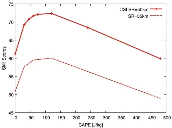
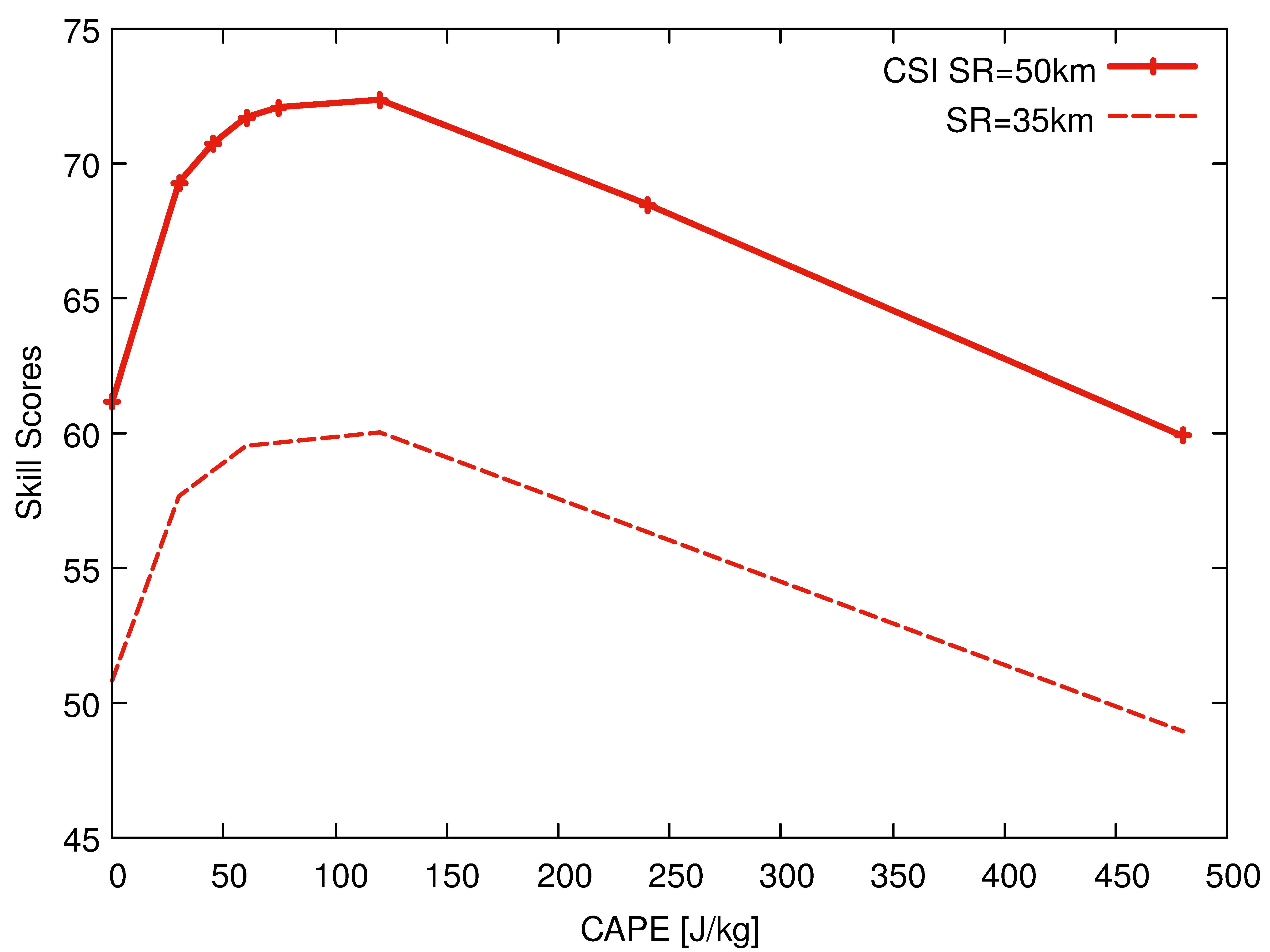
Skill scores (POD, FAR, CSI) in % plotted against CAPE for the 2016 period and a SR of 50 and 35 km, respectively. (Left) POD and FAR decrease with increasing CAPE. However, the decrease in POD is almost linear, whereas, FAR shows a strong decrease for low CAPE values up to a value of about 80. Then, FAR decreases only slightly with a tendency of getting constant for large CAPE values. (Right) This leads to the typical form of CSI. Strong increase for low CAPE values up to a maximum and an almost linear and moderate decrease afterwards.
Figure 5.
Skill scores (POD, FAR, CSI) in % plotted against CAPE for the 2016 period and a SR of 50 and 35 km, respectively. (Left) POD and FAR decrease with increasing CAPE. However, the decrease in POD is almost linear, whereas, FAR shows a strong decrease for low CAPE values up to a value of about 80. Then, FAR decreases only slightly with a tendency of getting constant for large CAPE values. (Right) This leads to the typical form of CSI. Strong increase for low CAPE values up to a maximum and an almost linear and moderate decrease afterwards.
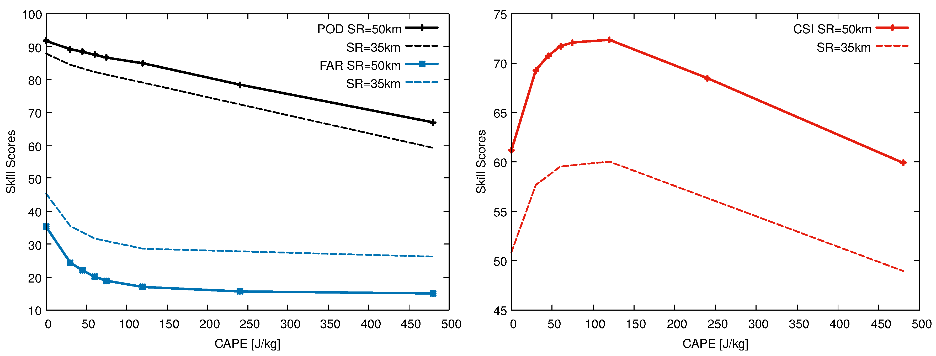
Figure 6.
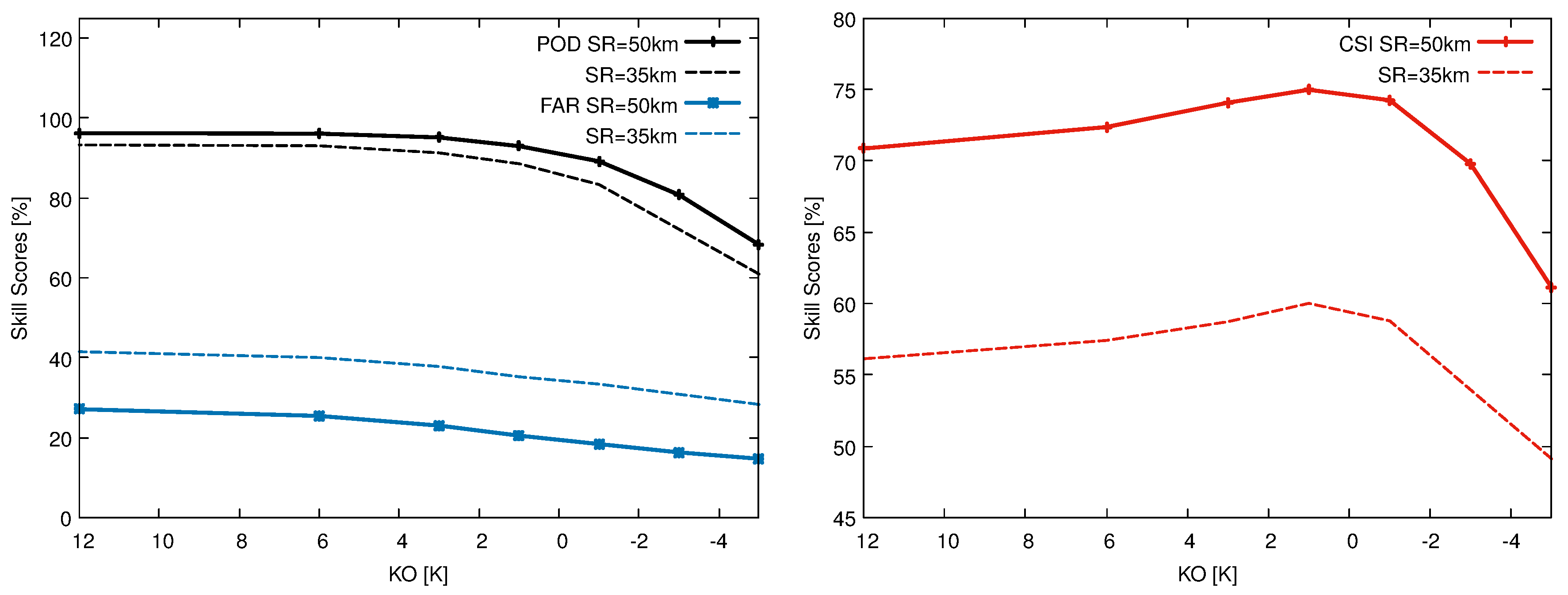
Skill scores (POD, FAR, CSI) plotted against KO for the 2017 period and a SR of 50 and 35 km, respectively. (Left) POD and FAR decrease with increasing CAPE. The form of FAR and POD is different compared to CAPE, resulting from the different definition of these variables. (Right) Again the relation between POD and FAR leads to a typical form of CSI. Strong increase for low (negative) KO values up to a maximum and an moderate decrease afterwards. Please note, the results for KO = −3 were not available for the SR35 plot.
Figure 6.
Skill scores (POD, FAR, CSI) plotted against KO for the 2017 period and a SR of 50 and 35 km, respectively. (Left) POD and FAR decrease with increasing CAPE. The form of FAR and POD is different compared to CAPE, resulting from the different definition of these variables. (Right) Again the relation between POD and FAR leads to a typical form of CSI. Strong increase for low (negative) KO values up to a maximum and an moderate decrease afterwards. Please note, the results for KO = −3 were not available for the SR35 plot.


Table 1.
Results of the different experiments. means the difference of infrared (IR) channels, whereby means that of the the water vapor channels, otherwise the channels are explicitely noted. Numerical Weather Prediction (NWP)/period provides the model used for NWP filtering and whether the investigated summer period was in 2016 or 2017. IFS is the forecast model of ECMWF and ICON of DWD. The other columns provide the probability of detection (POD), false alarm rate (FAR) and the critical success index (CSI).
| Nr | Experiment Settings: Cb If | NWP/Period | POD (%) | FAR (%) | CSI (%) |
|---|---|---|---|---|---|
| 1 | > −1 K and CAPE > 60 or TX > 50 | IFS/2016 | 87.5 | 20.1 | 71.7 |
| 2 | > −1 K, without NWP filtering | none/2016 | 91.6 | 35.2 | 61.1 |
| 3 | −2 K and CAPE > 60 or TX > 50 | IFS/2016 | 93.1 | 26.9 | 69.3 |
| 4 | > −2 K, without NWP filtering | none/2016 | 96.4 | 46.4 | 52.5 |
| 5 | > −1 K and CAPE > 60 or TX > 50 or > 6 K | IFS/2016 | 90.0 | 25.4 | 68.9 |
| 6 | > −1 K and CAPE > 60 or TX > 50 or > 8 K | IFS/2016 | 89.2 | 21.6 | 71.6 |
| 7 | > 224 K and CAPE > 60 or TX > 50 | IFS/2016 | 86.5 | 21.5 | 70.0 |
| 8 | > −1 K and CAPE > 60 | IFS/2016 | 86.2 | 19.7 | 71.1 |
| 9 | > −1 K and CAPE > 60 | ICON/2016 | 86.3 | 18.8 | 71.9 |
| 10 | > −1 K and CAPE > 60 | ICON/2017 | 90.1 | 19.0 | 74.4 |
| 11 | > −1 K and KO < 3 | ICON/2017 | 95.1 | 22.8 | 74.1 |
| 12 | > −1 K and KO < 3 or CAPE > 60 | ICON/2017 | 95.1 | 23.4 | 73.7 |
| 13 | > −1 K, without NWP filtering | ICON/2017 | 96.2 | 27.5 | 70.5 |
© 2018 by the authors. Licensee MDPI, Basel, Switzerland. This article is an open access article distributed under the terms and conditions of the Creative Commons Attribution (CC BY) license (http://creativecommons.org/licenses/by/4.0/).
Share and Cite
MDPI and ACS Style
Müller, R.; Haussler, S.; Jerg, M. The Role of NWP Filter for the Satellite Based Detection of Cumulonimbus Clouds. Remote Sens. 2018, 10, 386. https://doi.org/10.3390/rs10030386
AMA Style
Müller R, Haussler S, Jerg M. The Role of NWP Filter for the Satellite Based Detection of Cumulonimbus Clouds. Remote Sensing. 2018; 10(3):386. https://doi.org/10.3390/rs10030386
Chicago/Turabian StyleMüller, Richard, Stephane Haussler, and Matthias Jerg. 2018. "The Role of NWP Filter for the Satellite Based Detection of Cumulonimbus Clouds" Remote Sensing 10, no. 3: 386. https://doi.org/10.3390/rs10030386
Note that from the first issue of 2016, this journal uses article numbers instead of page numbers. See further details here.