Classifying Wheat Hyperspectral Pixels of Healthy Heads and Fusarium Head Blight Disease Using a Deep Neural Network in the Wild Field

Abstract

Classification of healthy and diseased wheat heads in a rapid and non-destructive manner for the early diagnosis of Fusarium head blight disease research is difficult. Our work applies a deep neural network classification algorithm to the pixels of hyperspectral image to accurately discern the disease area. The spectra of hyperspectral image pixels in a manually selected region of interest are preprocessed via mean removal to eliminate interference, due to the time interval and the environment. The generalization of the classification model is considered, and two improvements are made to the model framework. First, the pixel spectra data are reshaped into a two-dimensional data structure for the input layer of a Convolutional Neural Network (CNN). After training two types of CNNs, the assessment shows that a two-dimensional CNN model is more efficient than a one-dimensional CNN. Second, a hybrid neural network with a convolutional layer and bidirectional recurrent layer is reconstructed to improve the generalization of the model. When considering the characteristics of the dataset and models, the confusion matrices that are based on the testing dataset indicate that the classification model is effective for background and disease classification of hyperspectral image pixels. The results of the model show that the two-dimensional convolutional bidirectional gated recurrent unit neural network (2D-CNN-BidGRU) has an F1 score and accuracy of 0.75 and 0.743, respectively, for the total testing dataset. A comparison of all the models shows that the hybrid neural network of 2D-CNN-BidGRU is the best at preventing over-fitting and optimize the generalization. Our results illustrate that the hybrid structure deep neural network is an excellent classification algorithm for healthy and Fusarium head blight diseased classification in the field of hyperspectral imagery.

1. Introduction

Fusarium head blight disease is not evenly distributed across a wheat field, but occurs in patches with large areas of the field free of disease in the early stages of infestation, which will eventually result in significant losses. Fusarium head blight is an intrinsic infection by fungal organisms, after infestation, this disease can harm the normal physiological function of wheat, and cause changes in the form and internal physiological structure [1,2,3]. After the wheat is infected, several fungal toxins will be produced. Deoxynivalenol (DON) is the most serious of these toxins. DON can lead to poisoning in people or animals and persists in the food chain for a long time [4,5]. If the disease in the field can be detected earlier and quicker, wheat containing the toxins can be isolated, which can reduce the loss caused by disease. Scabs appear on the wheat head due to chlorophyll content degradation and water losses after the wheat is infected [6,7]. Digital image and spectral analysis can be applied to detect the disease. The spectral reflectance of diseased plant tissue can be investigated as a function of the change in plant chlorophyll content, water, morphology, and structure during the development of the disease [8,9].

Hyperspectral imagery technology is a non-invasive method and consumes large amounts of memory and tranmission bandwidth, so that the very large data cubes can extract features and spectral identification, which represents a small subset. Hyperspectral imagery can include the spectral, spatial, textural, and contextual features of food and agricultural products [10,11,12]. In addition, the application of hyperspectral imagery detection for wheat disease is relatively recent and offers interesting and potentially discerning opportunities [13]. The occurrence Fusarium head blight disease is a short time, and lasts approximately half of a month. Since the field environment has a strong influence on hyperspectral imagery, previous studies have mainly focused on laboratory conditions [14]. Bauriegel detected the wavelength of the Fusarium infection in wheat using hyperspectral imaging via Principal Component Analysis (PCA) under laboratory conditions. The degree of disease was correctly classified (87%) in the laboratory by utilizing the spectral angle mapper. Meanwhile, the medium milk stage was found to be the best time to detect the disease using spectral ranges of 665–675 nm and 550–560 nm [14]. Karl-Heinz Dammer used the normalized differential vegetation index of the image pixels and the threshold segmentation to discriminate between infected and non-infected plant tissue. The grey threshold image of the disease ear shows a linear correlation between multispectral images and visually estimated disease levels [15]. However, multispectral and RGB imagery are used to detect only infected ears with typical symptoms via sophisticated analysis of the image under uniform illumination conditions. Spectroscopy and imaging platforms for tractors, UAVs, aircraft and satellites are current innovative technologies for mapping disease in wild fields [16].

The hyperspectral imagery classification model must be robust and generalizable to improve the disease detection accuracy in wild fields. The traditional commonly used algorithm is a Support Vector Machine (SVM), which has achieved remarkable results in statistical process control applications [17]. Qiao uses the method of SVM to classify fungi-contaminated peanuts in hyperspectral image pixels, and the classification accuracy exceeded 90% [18]. When using SVM to classify hyperspectral images, the spectral and spatial features should be extracted with reduced dimensionality. The overall accuracy increased from 83% without any feature reduction to 87% with feature reduction based on several principal components and morphological profiles [19]. Feature reduction can be seen as a transformation from high dimensions to low dimensions to overcome the curse of dimensionality, which is a common phenomenon when conducting analyses in high-dimensional space. For a given number of available training samples, the curse of dimensionality decreases the classification accuracy as the dimensions of the input feature vectors increase [20]. Therefore, the analysis of hyperspectral images that are large data cubes faces the major challenge of addressing redundant information.

The method of deep learning originates from an artificial neural network, the Multiple Layer Perceptron (MLP). Among the several applications of deep neural networks, Deep Convolutional Neural Nets (DCNN) have brought about breakthroughs in processing images, face detection, audio, and so on [21,22,23]. In 2015, DCNN is firstly introduced into hyperspectral images classification And Wei Hu also proposed convolutional layers and max pooling layer to discriminate each spectral signature [24,25]. DCNN shows excellent performance for hyperspectral image classification [26], including cancer classification [27], and land-cover classification [28]. A Deep Recurrent Neural Network (DRNN), another typical deep neural network, is a sequence network that contains the hidden layers and memory cells to remember the sequence state [29,30]. In 2017, Li was the first use the DRNN to treat the pixels of hyperspectral image as the sequence data. They developed a novel function, named PRetanh, for hyperspectral imagery [31]. In addition, the deep convolutional recurrent neural network for hyperspectral image was firstly for hyperspectral images that were used by Hao Wu in 2017. They constructed a few convolutional layers and followed recurrent layers to extract the contextual spectra information using the features of the convolutional layers. By combining convolutional and recurrent layers, the DCRNN model achieves results that are superior to those of other methods [32].

Up to now, research on wheat Fusarium infection was primarily focused on approaches to classify the fungal disease of wheat kernels by grey threshold segmentation, or extract head blight symptoms based on PCA [33,34,35]. In the early development stage of Fusarium head blight disease, infected and healthy grains are easier to separate, but the disease symptoms are difficult to diagnose. [14,15]. Moreover, in a wild field, the complicated environmental conditions and irregular disease patterns limit the classification accuracy of hyperspectral imagery experiments.

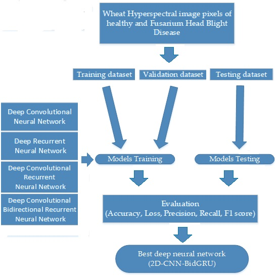
Therefore, the current study’s main aim is to develop a robust and generalizable classification model for hyperspectral image pixels to detect early-stage Fusarium head blight disease in a wild field. Specifically, the main work are listed, as follows.

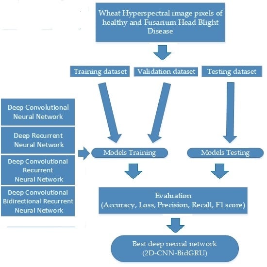
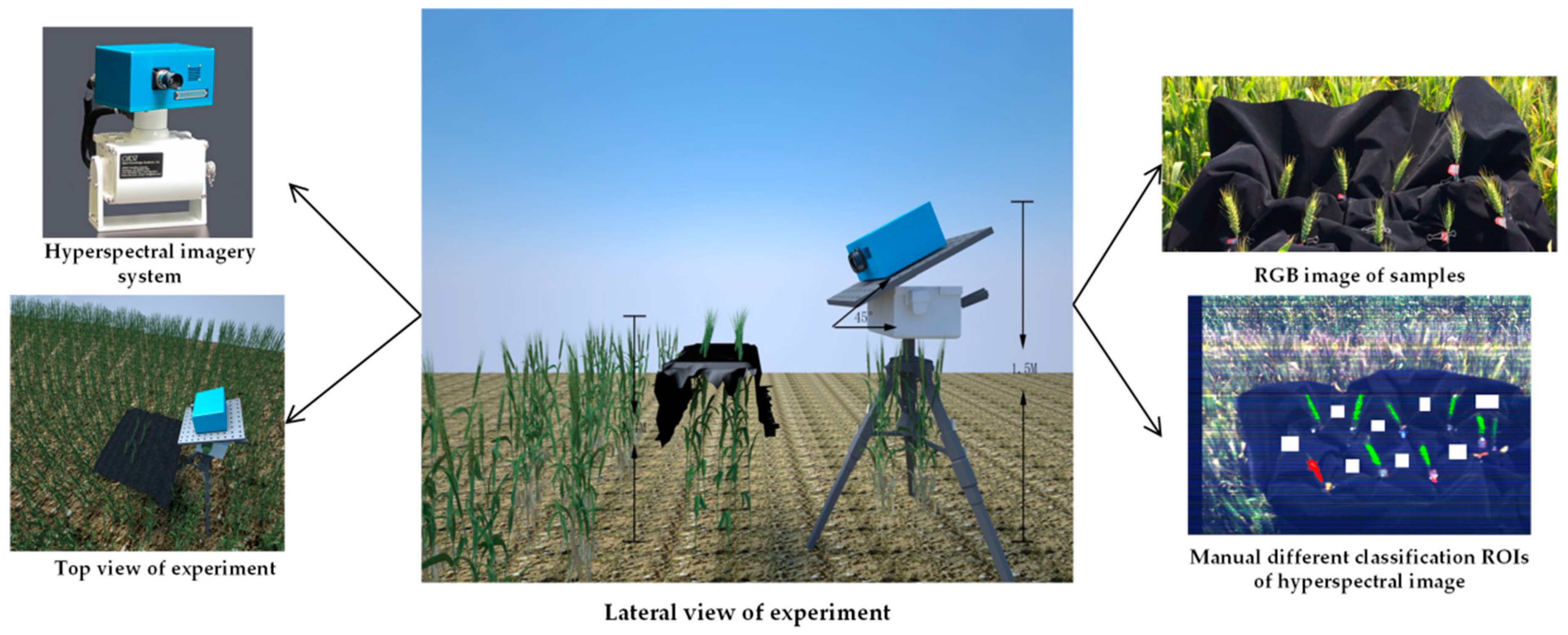
• Design and complete a hyperspectral image classification experiment for healthy head and Fusarium head blight disease in the wild field. The hyperspectral images are divided by pixels of different classes into a training dataset, a validation dataset, and a testing dataset to training the model.
• Compare and improve the different deep neural networks for hyperspectral image classification. These neural networks include DCNN with two input data structures, DRNN with Long Short Term (LSTM), and the Gated Recurrent Unit (GRU), and an improved hybrid CRNN.
• Take advantage of these assessment methods to determine the best model for classifying hyperspectral image pixels. Different SVM and deep neural network models are assessed and analysed on training dataset, validation dataset, and the testing dataset.

The remainder of this paper is organized as follows. An introduction to the experiment for obtaining hyperspectral imagery of Fusarium head blight disease is briefly given in Section 2. The details of the classification algorithms, including modeling and evaluating, are described in Section 3. The experimental results and a comparison with different approaches are provided in Section 4. Section 5 discusses the effectiveness of the early diagnosis of Fusarium head blight disease by different hyperspectral classification models; finally, Section 6 concludes this paper.

2. Materials and Methods

2.1. Plant Material

The field wheat plants were grown in Guo He town, Hefei City, Anhui Province, China, in 2017. The occurrence of disease is completely naturals because the cultivation process does not utilize pesticides, which guarantees the success of cultivation and illustrates the real and typical symptoms of Fusarium head blight of wheat. To ensure the quality of the experimental data, the period of the experiment from 29 April to 15 May in 2017 is the ideal time for disease detection from the wheat from the medium milk stage to the fully ripe stage for obtain the real and valid hyperspectral images. Several factors influence the hyperspectral imagery experiment, including wind, humidity, and temperature, and the best experimental time of day is noon because of the suitable sunbeam angle. The constraining factors of the environment were considered in the experiment, and 90 samples of wheat ear were divided into 10 regions, with a hyperspectral image acquired for each region. Analysis of the hyperspectral image indicated that by 9–10 May, the early period of the disease development were stable (29 $\pm$ 2 °C, humidity 70%, breeze), and three groups of wheat hyperspectral images were selected in consideration of the prominent disease appearance.

2.2. Experiment Apparatus and Procedure in the Field

Following the consideration of the complexity of the field environment, the field experiment was devised to improve the program of measurement in Figure 1, which shows that the hyperspectral image data of Fusarium head blight disease was acquired with a hyperspectral VNIR system and auxiliary equipment in the field. The system consisted of the following parts: a pushbroom-type hyperspectral apparatus (OKSI, Torrance, CA, USA), a rotation stage with a pan/tilt head for scanning, a Dell Precision Workstation with the data collection software HyperVision (OKSI, Torrance, CA, USA), and a set of height-adjustable mounting brackets. Wheat samples were placed in a fixed region, and a piece of black light-absorbing cloth was placed under the targeted object as the background. The lateral view of the experiment shows the basic setting:

• the tripod apparatus is placed about 30 cm in front of these samples;
• the high spectral camera adjusts to a height of 1.5 m from the ground
• the cloud platform is 45 degrees in the horizontal direction;
• the scan range is −30 degrees to +30 degrees; and,
• the measurement times were set from 11:00 a.m. to 2:00 p.m. to acquire sufficient light.

Figure 1 shows an RGB image of nine wheat heads of each hyperspectral image. The outputs of this system were “image cubes” of wheat heads region consisting of a two-dimensional spatial image (1620 × 2325 pixels) with spectral data (400–1000 nm and 1.79 nm resolution, 339 wavebands) at each pixel. The pixel spectra classes are background, healthy, and diseased. The reflectance of the pixel spectra was derived using of standard method of a white panel (Lab sphere, North Sutton, NH, USA). Digital Numerical (DN) is the uncalibrated value of the hyperspectral imaging system. DN_T is the DN of a diseased sample, and DN_W is the DN of a white panel. DN_B is the DN that is invoked as a substitute for dark current and noise when the camera shutter closed. The reflectance R can be calculated from the following equation [36]:

$$\mathrm{R}=\frac{{\mathrm{DN}}_{\mathrm{T}}-{\mathrm{DN}}_{\mathrm{B}}}{{\mathrm{DN}}_{\mathrm{W}}-{\mathrm{DN}}_{\mathrm{B}}}\times 100\%$$

(1)

The hyperspectral image data were analysed with ENVI (Environment for Visualizing Images) software of the Exelis Visual Information Solutions Company. The Fusarium head blight disease is visually distinguished by false colour images in Figure 1. False colour images also facilitated the proper manual setting of the Region Of Interst (ROI) and the selection of tissues for spectral analysis. Additionally, the ENVI software can use the manual fraction to increase the ROI of the wheat head.

3. Model Analysis

3.1. The Deep Convolutional Neural Network

For deep models, DCNN is widely used as a feed-forward neural network consisting of a convolution layer, a pooling layer, and a fully connected layer [37,38]. The unit of the convolution layer is the feature graph, and each unit is related to the block of the previous feature graph by the filter group. The pooling layer takes a specific value as the output value in a small area. The main purpose of the pooling operation is to reduce the dimension [39]. The one-dimension convolution neural network (1D-CNN) has been successfully used for hyperspectral image pixel-level classification [40,41]. A spectral vector of the hyperspectral image pixel is taken as the input layer. Analogous to the 1D-CNN, the two-dimension convolution neural network (2D-CNN) is widespread for two-dimensional image data.

There is a comparison between the one-dimensional pixel vector and the two-dimensional gray-scale image, which is based on spectral information in Figure 2. For the neural network of the model, the convolutional layer and pooling layer refer to the Visual Geometry Group neural network (VGG network) [42], the kernel is 3 × 3, and the pooling layer is 2 × 2. The significant improvement of the VGG network makes the neural network deeper and uses two 3 × 3 kernels instead of a 5 × 5 kernel, which decreases the number of parameters and the amount of computation. By contrast to the configuration of the VGG network, the kernel sizes of 1D-CNN and 2D-CNN are 3 and 3 × 3, respectively.

Table 1. One-dimension convolution neural network (1D-CNN) and two-dimensional convolutional neural network with gated recurrent unit (2D-CNN) configurations.

CNN Configuration
1D-CNN	2D-CNN
Input (256 × 1) Spectrum	Input (16 × 16) Spectrum
Convolution 3–64	Convolution 3.3–64
Convolution 3–64	Convolution 3.3–64
Maxpooling 2	Maxpooling 2.2
Convolution 3–64	Convolution 3.3–64
Convolution 3–64	Convolution 3.3–64
Maxpooling 2	Maxpooling 2.2
FC Dense	FC Dense
Softmax	Softmax

shows the configuration of the 1D-CNN and 2D-CNN, which both use four convolutional layers, two pooling layers, one dense layer for the deep neural network, and the dropout function to prevent the over-fitting.

3.2. Deep Recurrent Neural Network

A DRNN is a classic framework for time sequence data that is different from the convolutional feed-forward neural network [43,44]. In a deep recurrent network, the output neuron can directly affect itself the next time. The original RNN has problems with gradient vanishing and gradient explosion. LSTM is a traditionally gated framework that is extended to the RNN to solve these problems, and GRU is a novelty gated framework.

LSTM was introduced by Hochreiter and Schmidhuber [45]. Graves reviewed and utilized the LSTM to generate and recognize speech [46,47]. LSTM consists of three gates (i.e., a forget gate, an input gate, and an output gate). “h” is the prior output. ”x” is the current input. ”$\sigma$” is the sigmoid function. “b” is the bias item.

The forget gate formula is:

$$f_t=\sigma \left(W_f\cdot \left[h_{t-1},X_t\right]+b_f\right)$$

(2)

The input gate formula is:

$$\begin{array}{c}{i}_t=\sigma \left(w_i\cdot \left[h_{t-1},x_t\right]+b_i\right)\\ \tilde{C}=tanh\left(w_c\cdot \left[h_{t-1},x_t\right]+b_c\right)\\ C_t=f_t*C_{t-1}+i_t*\widetilde{C_t}\end{array}$$

(3)

The ‘tanh’ function creates a new candidate “C”; “i” is the selection result for “C”; the “C_t” uses “C_t−1”, “f_t“, and “$\tilde{C}$” to update the state.

The output gate formula is:

$$\begin{array}{c}{o}_t=\mathsf{\sigma }\left(W_o\left[h_{t-1},x_t\right]+b_o\right)\\ h_t=o_t*\tan \mathrm{h}\left(C_t\right)\end{array}$$

(4)

GRU is the optimal form of the LSTM architecture to adaptively capture dependencies of different time scales [48,49]. The GRU has an update gate, and an input gate. These gates’ formulas are:

$$\begin{array}{c}\begin{array}{c}{z}_t=\mathsf{\sigma }\left(W_z\left[h_{t-1},x_t\right]+b_t\right)\\ r_t=\mathsf{\sigma }\left(W_r\left[h_{t-1},x_t\right]+b_t\right)\\ \widetilde{h_t}=tanh\left(W\cdot \left[r_t*h_{t-1},x_t\right]+b_t\right)\end{array}\\ h_t=\left(1-z_t\right)*h_{t-1}+z_t*\widetilde{h_t}\end{array}$$

(5)

Two RNN models with three stacked LSTM layers and GRU layers, respectively, are able to learn higher-level temporal representations, as shown in

Table 2. LSTM and Gated Recurrent Unit (GRU) configurations.

RNN Configuration
LSTM	GRU
Stacked LSTM 64	Stacked GRU 64
Stacked LSTM 64	Stacked GRU 64
Stacked LSTM 64	Stacked GRU 64
Softmax	Softmax

.

3.3. Deep Convolutional Recurrent Neural Network

To take advantage of characteristics of the convolutional and recurrent layers, a deep convolutional recurrent neural network (DCRNN) integrates a convolutional layer with a recurrent layer as a complete framework for the classification of images, language, and so on [50]. The DCRNN can learn better image representation, because the convolutional layers act as feature extractors and provide abstract representations of the input data in feature maps, and the recurrent neural networks are designed to learn contextual dependencies by using the recurrent connections [50,51]. Because the feature of a different wavelength is a mutual correlation, such as the vegetation index, the hybrid neural network structure can extract features of spectra sequences from the convolutional layer, and then obtain the contextual information of the feature from the recurrent layer. The training process of the hybrid model may draw from deeper and useful characteristics of hyperspectral image pixels. The framework of DCRNN consists of three parts: convolution layers, a reshape layer to change the tensor dimensions, and three stacked recurrent layers, using LSTM or GRU.

To improve the generalizability, a bidirectional RNN includes forward and backward features of the spectra from Equation (6). The hybrid structure can be utilized for natural language processing and phonetic recognition [52]. The bidirectional LSTM network was proposed for sequence tagging and other fields [53,54]. In 2017, hyperspectral image classification first used the bidirectional LSTM of CRNN, and the accuracy of the training dataset was over 95% [32]. A bidirectional GRU that exploited the context to resolve ambiguities better than the unidirectional GRU was utilized to extract efficient features and make the classifier perform better than the unidirectional method [55,56].

The formula of the bidirectional RNN is:

$$\begin{array}{c}{\overrightarrow{h}}_t^{\left(i\right)}=f({\overrightarrow{W}}_{}^{\left(i\right)}{h}_t^{\left(i-1\right)}+{\overrightarrow{V}}_{}^{\left(i\right)}{h}_t^{\left(i\right)}+{\overrightarrow{b}}^{\left(i\right)})\\ {\overleftarrow{h}}_t^{\left(i\right)}=f({\overleftarrow{W}}_{}^{\left(i\right)}{h}_t^{\left(i-1\right)}+{\overleftarrow{V}}_{}^{\left(i\right)}{h}_t^{\left(i\right)}+{\overleftarrow{b}}_{}^{\left(i\right)})\\ y_t=g(U[{\overrightarrow{h}}_t^{\left(i\right)};{\overleftarrow{h}}_t^{\left(i\right)}]+c)\end{array}$$

(6)

Therefore, the hybrid structure use the bidirectional LSTM and bidirectional GRU, instead of the LSTM and GRU, and Figure 3 shows that the feature of the convolutional layers can flow into the recurrent layers to capture the global information for hyperspectral images.

Table 3. Deep convolutional recurrent neural network (DCRNN) configuration.

DCRNN Configuration
2D-CNN-LSTM	2D-CNN-GRU	2D-CNN-BidLSTM	2D-CNN-BidGRU
Input (16 × 16)	Input (16 × 16)	Input (16 × 16)	Input (16 × 16)
Convolution 3.3–64	Convolution 3.3–64	Convolution 3.3–64	Convolution 3.3–64
Convolution 3.3–64	Convolution 3.3–64	Convolution 3.3–64	Convolution 3.3–64
Maxpooling 2.2	Maxpooling 2.2	Maxpooling 2.2	Maxpooling 2.2
Convolution 3.3–64	Convolution 3.3–64	Convolution 3.3–64	Convolution 3.3–64
Convolution 3.3–64	Convolution 3.3–64	Convolution 3.3–64	Convolution 3.3–64
Maxpooling 2.2	Maxpooling 2.2	Maxpooling 2.2	Maxpooling 2.2
Reshape layer	Reshape layer	Reshape layer	Reshape layer
Stacked LSTM 64	Stacked GRU 64	Stacked Bidirectional LSTM 64	Stacked Bidirectional GRU 64
Stacked LSTM 64	Stacked GRU 64	Stacked Bidirectional LSTM 64	Stacked Bidirectional GRU 64
Stacked LSTM 64	Stacked GRU 64	Stacked Bidirectional LSTM 64	Stacked Bidirectional GRU 64
Softmax	Softmax	Softmax	Softmax

presents four hybrid models, namely, a two-dimensional convolutional neural network with long short-term memory (2D-CNN-LSTM), a two-dimensional convolutional neural network with gated recurrent unit (2D-CNN-GRU), a two-dimensional convolutional neural network with bidirectional long short-term memory (2D-CNN-BidLSTM), and a two-dimensional convolutional neural network with a bidirectional gated recurrent unit (2D-CNN-BidGRU).

3.4. Evaluation Method

This paper considers the following criteria to select the best model. Accuracy is widely implemented for classified hyperspectral pixels. However, the accuracy is not sufficient for imbalanced datasets. The confusion matrix, viewed as an error matrix, can clearly depict the predicted categories for each row and the actual categories for each column. However, the confusion matrix cannot directly determine the evaluation of the classifier model. Therefore, we use precision, recall, and F1 score to assess these models.

TP, FP, FN, and TN stands for true positive, false positive, false negative, and true negative, respectively. The formulas of Precision (P) and Recall (R) are [57]:

$$\begin{array}{c}\mathrm{P}=\frac{\mathrm{TP}}{\mathrm{TP}+\mathrm{FP}}\\ \mathrm{R}=\frac{\mathrm{TP}}{\mathrm{TP}+\mathrm{FN}}\end{array}$$

(7)

The performance of models expect the value of precision and recall to be higher, but they are incompatible. The F1 score is a better metric that combines the characteristics of precision and recall to evaluate the model for different classes in the dataset. A good F1 score is also indicative of satisfactory classification performance. The F1 score formula is [57]:

$$\mathrm{F}1=\frac{2\mathrm{PR}}{\mathrm{P}+\mathrm{R}}=\frac{2\mathrm{TP}}{2\mathrm{TP}+\mathrm{FP}+\mathrm{FN}}$$

(8)

The Tensorflow framework with Python 3.5 is implemented on a workstation with a 3.5 GHz Intel(R) Core i7 CPU and a NVIDIA(R) GTX 1080TI GPU.

4. Results

4.1. Experiment Dataset and Analysis

The original data comprise hyperspectral image cubes for six sample regions in Figure 1. Three types are included: background pixels, healthy pixels, and the diseased pixels.

Table 4. The total number of ROI pixels.

Sample Name	Original Data (Pixel Number)
	Background	Health	Disease	Total
Sample 1 on the first day	30,821	85,777	13,917	130,515
Sample 2 on the first day	65,452	72,933	6517	144,902
Sample 3 on the first day	74,778	89,198	17,480	181,456
Sample 1 on the second day	10,535	29,001	24,635	64,171
Sample 2 on the second day	38,515	33,913	31,114	103,542
Sample 3 on the second day	64,105	81,521	38,988	184,614
Total	284,206	392,343	132,651	809,200

shows the number of these ROI pixels. The dataset suffers from the imbalance problem where the number of diseased pixels is obviously smaller than the numbers of healthy and background pixels. Sample class imbalance is a common problem that has a detrimental effect on classification performance. Several methods can be used to resolve the issue: oversampling, undersampling, and two-phase training [58,59,60]. To avoid sample quantity interference, we use undersampling to guarantee no difference in the numbers of samples of different types. After randomly undersampling the data, the total size of the training and validation datasets is 227,484. The total size of the testing dataset is 581,716.

When considering the dataset of deep model, the spectra of hyperspectral image pixel will be reshaped into the two dimensional data as grey image. There are many preprocessing methods for image data of deep model, such as normalization, mean-removal, and PCA whitening. Preprocessing methods could speed up the gradient descent and improve the accuracy. PCA whitening is mainly used into the dimensionality reduction with colour image [61]. But, this input data for these deep models is similar to grey image. Therefore, the preprocessing method of spectra samples uses the mean-removal method that can be used to reduce the sampling error from different experiment dates [62].

PCA method that can identify the principal characteristics of the data at different observation times can be used to improve the visualization of spectra data to compare the mean-removed and non-mean-removed data [63,64,65]. In Figure 4, the red discrete points are the first-day samples, and the yellow discrete points are the second-day samples. The discrete points in Figure 4a show 800 random background, healthy, and diseased pixels, that are clearly irrelevant from different observation times. In Figure 4b, first-and second-day discrete points show more obvious overlap, especially the background samples. The illustration shows that the spectra from different experiment dates don’t belong to the same range of values, and mean-removal reduces the difference between the first- and second-day samples. The last step of preprocessing is normalization, which is a conventional method for deep learning [23].

4.2. Model Training

When training models, the data set is divided into a training set (70%) and a validation set (30%). The training results are used to search the hyperparameters of the deep neural network. In our experiments, the loss function is “cross entropy” [66,67]; the optimizer is “adadelta” [68,69]; the activation function is “elu” for the convolutional layer and the dense layer and the “tanh” for the recurrent layer; the batch size is 64 [44,70]; and, the regularization and dropout function are used to decrease over-fitting [71,72]. In terms of accuracy and loss, a number of deep neural networks are regular and stabilized after 300 epochs of training.

Figure 5 shows the accuracy and loss of models of the training dataset and validation dataset after 300 epochs. Figure 5a,b show the training accuracy and loss of 1D-CNN and 2D-CNN, which have similar networks, and contrast 1D-CNN with 2D-CNN, which reshape the dimension into 16 × 16 grey images for the input layer. The results indicate that two models have equivalent accuracy and loss for the training dataset, whereas for validation dataset, the accuracy and loss of 2D-CNN are better than those of 1D-CNN. Figure 5c,d show the training result of LSTM and GRU. The recurrent neural network of LSTM and GRU both have over-fitting problems in terms of accuracy and loss in the training dataset and the validation dataset, but GRU is better than LSTM in the preliminary training period.

Figure 5e–h compare the training and validation results of the hybrid structures 2D-CNN-LSTM, 2D-CNN-GRU, 2D-CNN-BidLSTM, and 2D-CNN-BidGRU. Figure 5e,f show that the first hybrid structure also suffers from over-fitting with LSTM and GRU, especially the 2D-CNN-LSTM, but they are still better than the model with the recurrent neural network. Based on these result, the second hybrid neural network is reconstructed with the bidirectional LSTM and GRU instead of LSTM and GRU; the new hybrid networks are called 2D-CNN-BidLSTM and 2D-CNN-BidGRU, respectively. On the basis of Figure 5g,h, the second hybrid deep neural networks avoid over-fitting, while simultaneously improving the performance.

According to the results of different deep neural networks in Figure 5, the models that minimized the loss for the validation dataset are considered to be the best.

Table 5. Accuracy and loss of the best models, and training time (h).

Method	RBF-SVM	1D-CNN	2D-CNN	LSTM	GRU	2D-CNN-LSTM	2D-CNN-GRU	2D-CNN-BidLSTM	2D-CNN-BidGRU
Training ACC	0.705	0.815	0.839	0.839	0.847	0.842	0.842	0.843	0.849
Validation ACC	0.706	0.811	0.830	0.812	0.82	0.830	0.838	0.840	0.846
Training Loss	- 1	0.439	0.384	0.373	0.356	0.370	0.372	0.369	0.355
Validation Loss	- 1	0.437	0.394	0.443	0.420	0.400	0.376	0.372	0.358
Epoch	- 1	75	299	124	84	62	250	252	269
Training time (h)	1.7	16	11.8	6.2	13	11.6	11.8	12	12.4

¹ SVM algorithm has a different loss value, and its epoch is none.

shows the training accuracy, validation accuracy, training loss, validation loss, epoch, and training time for each model. 2D-CNN-BidGRU, which has the minimum loss, is the best training model. On the basis of Table 5, we can conclude that the maximum training accuracy is 0.847 for the GRU model, but the maximum validation accuracy is 0.83 for the 2D-CNN model. Therefore, a model using only independent CNN or RNN is not sufficient for training the best hyperspectral image classification model. Moreover, different deep learning algorithms will take almost the same training time expect LSTM, but all of the deep models require a longer time than SVM.

4.3. Model Testing

The performance of the models should be assessed using different methods for the testing dataset. In this experiment, the testing dataset is approximately three times larger than the training dataset; therefore, the testing accuracy is important, especially for the generalization assessment, because the models will be applied to classify the hyperspectral image for large scale disease detection.

In Figure 6 and Figure 7, we calculate the confusion matrix, precision, recall, and F1 score of the testing dataset to evaluate all models and to determine the best models from the testing dataset based on generalizability. Figure 6 presents the confusion matrix for the detailed classification models of the testing dataset that contains the background class, healthy class, and diseased class. Note the relatively large size of the testing dataset and that the healthy testing dataset has a high misclassification rate for all models.

Figure 7 and

Table 6. Evaluation of testing dataset for different models.

Method	RBF-SVM	1D-CNN	2D-CNN	LSTM	GRU	2D-CNN-LSTM	2D-CNN-GRU	2D-CNN-BidLSTM	2D-CNN-BidGRU
F1-score (Background)	0.75	0.84	0.86	0.82	0.84	0.84	0.86	0.88	0.88
F1-score (Healthy)	0.53	0.66	0.67	0.66	0.69	0.7	0.69	0.71	0.71
F1-score (Diseased)	0.42	0.5	0.51	0.49	0.5	0.5	0.51	0.52	0.52
F1-score (Total)	0.6	0.71	0.72	0.7	0.72	0.73	0.73	0.75	0.75
Accuracy	0.61	0.703	0.720	0.689	0.710	0.713	0.724	0.737	0.743
Testing efficiency (pixels/s)	371	2281	4185	2810	2770	4215	4215	3658	3658

show the precision, recall, and F1 scores for three classes of datasets and all models, respectively, for the testing dataset. In Figure 7, the precision of the healthy class is the highest, the recall of the disease class is the highest, the precision of the disease class is the lowest, and the recall of the healthy class is the lowest. The total precision and the total-recall for 2D-CNN-BidLSTM and 2D-CNN-BidGRU are both the highest of these models. Therefore, the F1 scores of 2D-CNN-BidGRU and 2D-CNN-BidLSTM are the same as in Table 6.

The F1 scores and accuracy of the models indicate that RBF-SVM performs worse than the deep neural network models because the classification of SVM does not apply to a large number of samples. Based on this assessment, 2D-CNN-BidGRU and 2D-CNN-BidLSTM are efficient, but 2D-CNN-BidGRU is better than 2D-CNN-BidLSTM with respect to the accuracy of the disease and healthy classifications. The hybrid structure connecting the CNN with the bidirectional recurrent neural network is better than that of other deep models. Although deep learning takes a longer training time, deep model are faster than SVM in testing time, which is more important in practice from Table 6. The development of GPU makes the tolerable training and testing time of deep neural network.

4.4. Original Hyperspectral Image Mapping

Finally, the grey hyperspectral image (670 nm) in the range of 665–675 nm for the head blight index (HBI) [14] is used to compare the mapping of original hyperspectral image by different models. Figure 8 shows the grey images of the original hyperspectral images mapped by these models. The results indicate that although these models can classify the diseased and healthy wheat heads, instrument noise influences the accuracy of the classification.

5. Discussion

The main purpose of this work was to study classification algorithms of hyperspectral image pixels and analyse the performance of deep models for diagnosing Fusarium head blight disease in wheat. Previous studies attempted to classify the disease symptoms based on spatial and spectral features via machine learning algorithms [14,15]; for example, PCA [33,34,35], random forest, and SVM [17,18,19]. Recently, the study of deep algorithms for hyperspectral imagery has becomes increasingly intensive, such as DCNN [24,25,26,27], DRNN [31], and hybrid neural networks [32]. The complicated hybrid structure [50,51] of a bidirectional recurrent layer [53,54] will help to improve the generalization of the classification model for prediction in testing datasets. This study, therefore, indicates that the benefits that are gained from deep characteristics of the disease spectra and identifies the best hybrid model for the diagnosis of Fusarium head blight disease in the field.

5.1. Extracting and Representing Deep Characteristics for Disease Symptoms

For high-resolution spectral instrumentation, the number of bands obtained by hyperspectral images is greater than that by multispectral images [12]. Therefore, the valid features of hyperspectral image pixels for disease detection in wild fields are difficult to determine. Many classifiers of hyperspectral images are based on specific wavelet features or vegetation indices that are related to pathological characteristics [7,10]. Deep feature extraction for disease detection by deep neural networks in the spectral domain is presented to acquire deeper information from hyperspectral images [26].

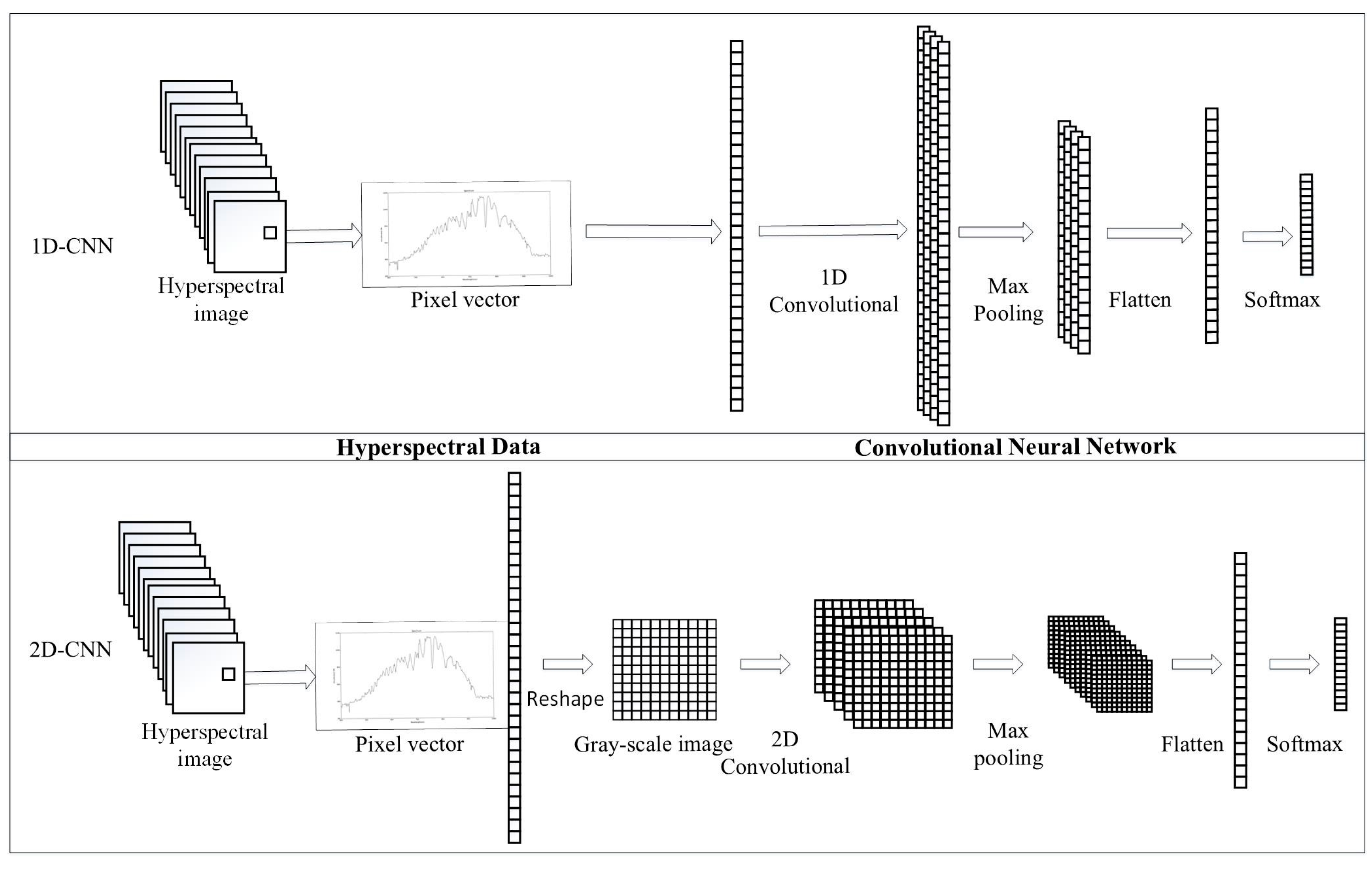
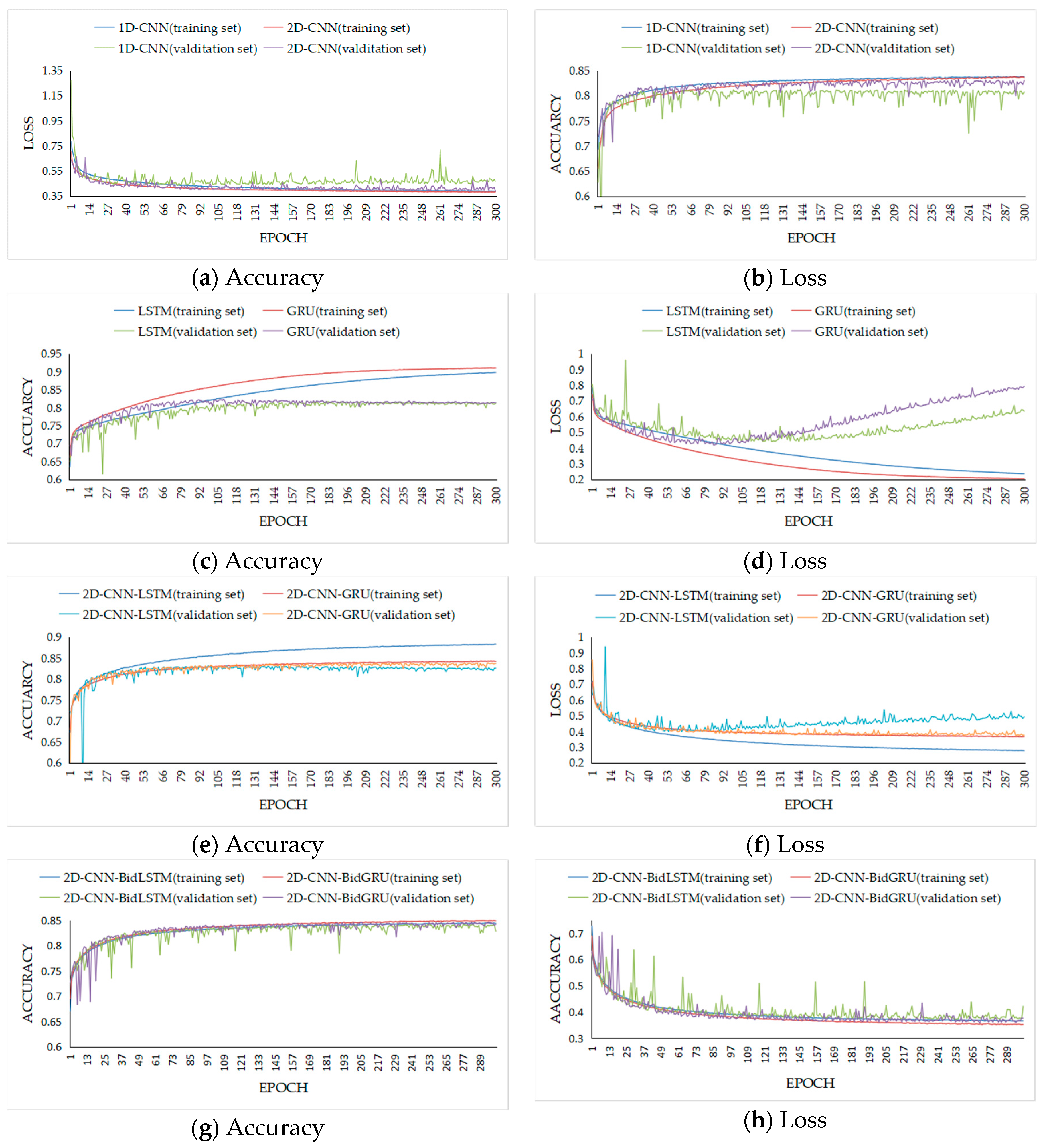
Among the abundance of deep learning methods, DCNN is commonly used to classify two-dimensional data-type images in visual tasks [42]. Our work on training and testing 1D-CNN and 2D-CNN shows that two-dimensional data can capture the intrinsic features of hyperspectral images better than one-dimensional data. 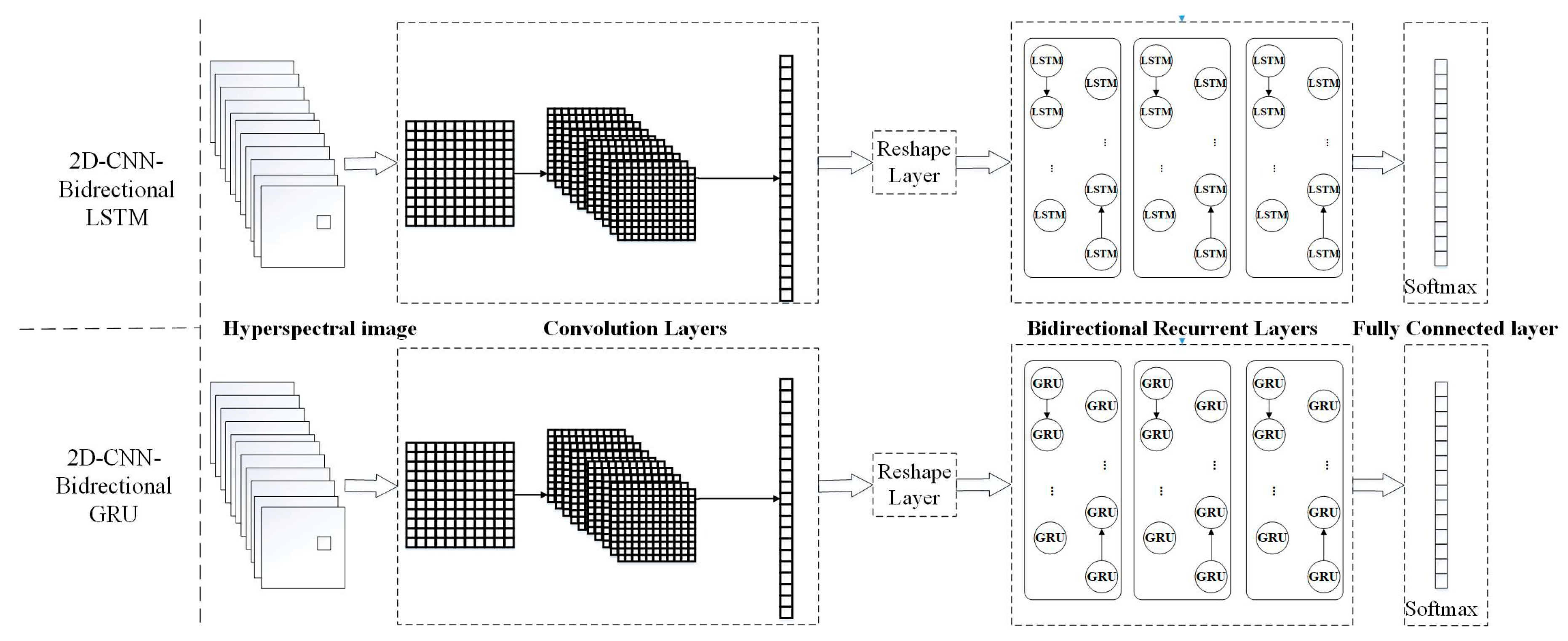Another significant branch of the deep learning family is the DRNN, which is designed to address sequential data [31]. By contrast to the CNN, the RNN maintains all of the spectral information in a recurrent procedure with a sequence-based data structure to characterize spectral correlation and band-to-band variability. As a result, to integrate the advantages of these deep neural networks, novel models that combine recurrent neural networks are proposed. However, in this work, the accuracy of second hybrid neural network with bidirectional recurrent layer for validation data is the better than first one with recurrent layer. The bidirectional RNNs that can incorporate contextual information from both past and future inputs [54]. The assessment results of all the deep models on the validation data show that 2D-CNN-BidGRU, with an accuracy of 0.846, is the most effective method for disease feature extraction from hyperspectral image pixels.

5.2. Assessing the Performance of Different Models for Hyperspectral Image Pixel Classification

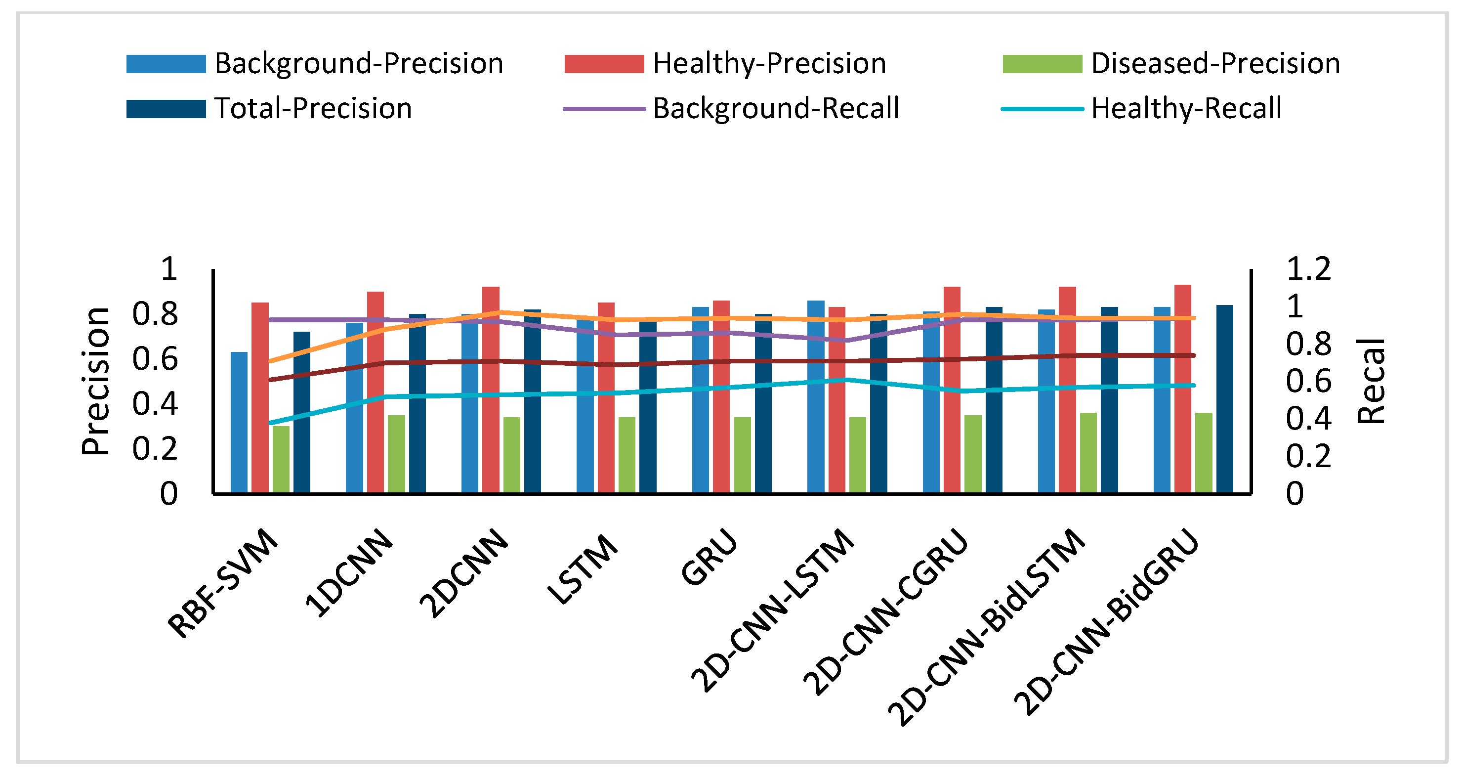
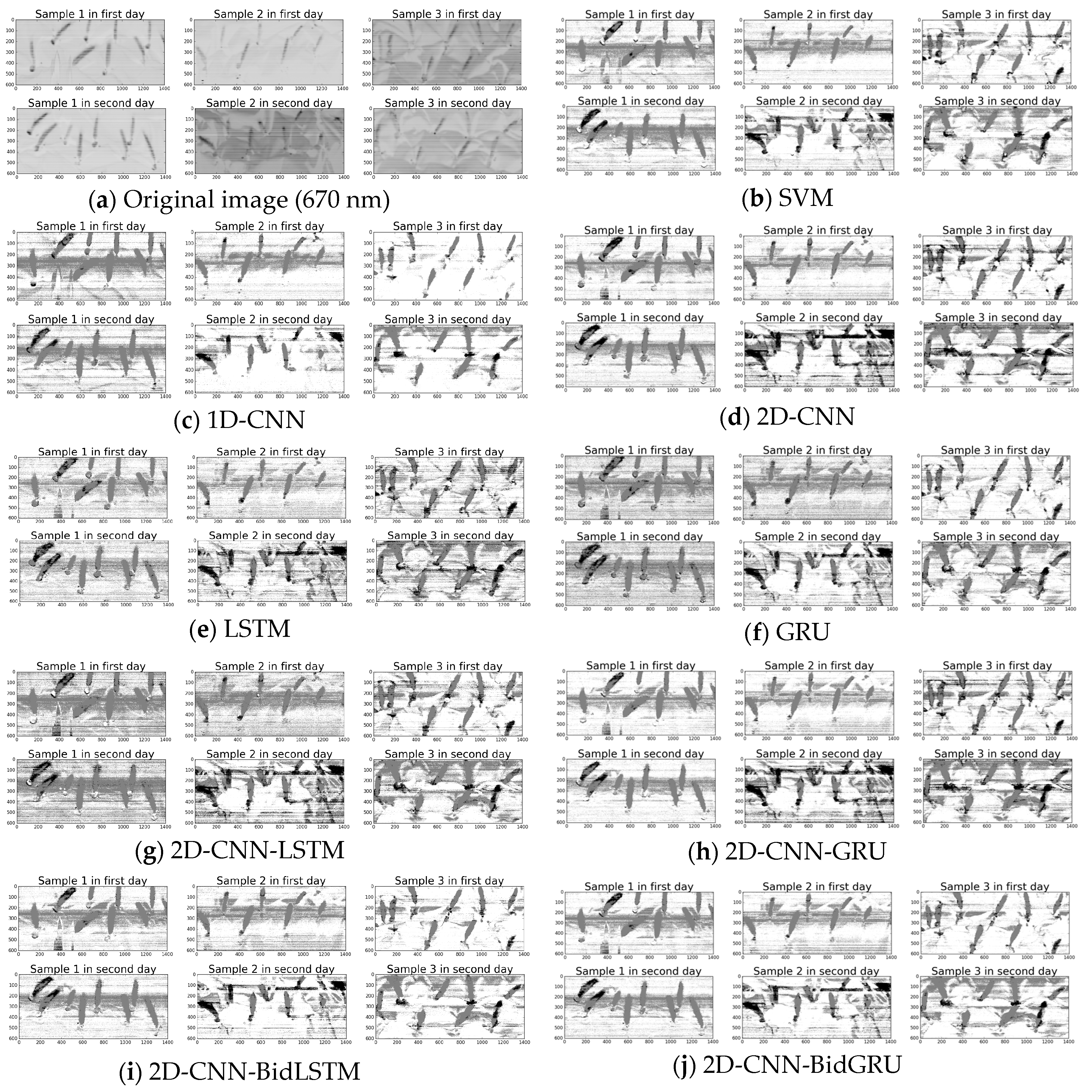
Robustness and generalizability are very important for large-scale disease detection in hyperspectral images. Therefore, the superior performance of a model must be assessed for a large number of testing datasets. The assessment metrics of these classification models include not accuracy, but the confusion matrix, F1 score, precision and recall [57]. The precision, recall, and F1 score for the testing dataset indicate that both the background and diseased classes are efficient for hyperspectral image pixel classification, but part of the healthy dataset is misclassified as diseased by all of the models.

The assessment results show that the deep models are better than SVM for the performance. With these deep models, despite applying regularization [71] and dropout [72] for the deep neural networks, the LSTM model, which has the worst performance, has an over-fitting problem. When a deep model learns a concept when there is noise in the training data, the problem of over-fitting will occur to such an extent that it negatively impacts the performance of the model on the testing data [73]. The performance of the hybrid neural networks are better than that of other deep neural networks. For comparing the assessment result of the two novel hybrid models on training and testing dataset, the first hybrid neural network with LSTM has the same over-fitting problem, but the second hybrid model with bidirectional LSTM and GRU can restrain the problem. The F1 score (0.75) and accuracy (0.743) on the testing dataset provide compelling evidence that the hybrid structure of 2D-CNN-BidGRU is the best for improving the model with respect to robustness and generalizability.

5.3. Next Steps

Notably, the application of deep neural networks to hyperspectral image pixel classification for Fusarium head blight disease is a new idea and has a great potential for disease diagnosis by remote sensing. Despite some insufficiencies, these results show that a deep neural network with a convolutional layer and bidirectional recurrent layer can classify the hyperspectral image pixels to diagnose the Fusarium head blight disease and improve the generalization and robustness of the classification model. In a wild wheat field, many types of objects have strong impacts on the generalization of the classification model. Therefore, future studies of deep models should apply more in-deep neural networks and customized loss functions to optimize these algorithms for a large number of testing datasets and more types of objects. Future study of application will focus on airborne hyperspectral remote sensing, which could be used to develop large-scale Fusarium head blight disease monitoring and mapping.

6. Conclusions

The study illustrates that deep neural networks can improve the classification accuracy and F1 score of Fusarium head blight disease detection from hyperspectral image pixels in a wild field. These results demonstrate that: (1) the hyperspectral image can be used to classify diseased and healthy wheat heads using the spectra of the pixels in a wild field; (2) the spectra of pixels can be reshaped into a two-dimensional data type to identify the features of disease symptoms more easily than using a one-dimensional data structure (3) when compared with other deep neural networks, the hybrid model of the convolutional bidirectional recurrent neural network can prevent over-fitting and achieve higher accuracy (0.846) on the validation dataset; and, (4) with a larger testing dataset, the 2D-CNN-BidGRU model has the best generalization performance that of F1 score and accuracy is 0.75 and 0.743, respectively. Our study provides a novel classification algorithm for the research on Fusarium head blight disease in a wild field within a complicated environment, which can be used in future studies of disease prediction and larger-scale disease assessment based on airborne hyperspectral remote sensing.

References

1. Karlsson, I.; Friberg, H.; Kolseth, A.K.; Steinberg, C.; Persson, P. Agricultural factors affecting Fusarium communities in wheat kernels. Int. J. Food Microbiol. 2017, 252, 53–60. [Google Scholar] [CrossRef] [PubMed]
2. Steiner, B.; Buerstmayr, M.; Michel, S.; Schweiger, W.; Lemmens, M.; Buerstmayr, H. Breeding strategies and advances in line selection for Fusarium head blight resistance in wheat. Trop. Plant Pathol. 2017, 42, 165–174. [Google Scholar] [CrossRef]
3. Šíp, V.; Chrpová, J.; Štěrbová, L.; Palicová, J. Combining ability analysis of fusarium head blight resistance in European winter wheat varieties. Cereal Res. Commun. 2017, 45, 260–271. [Google Scholar] [CrossRef]
4. Palacios, S.A.; Erazo, J.G.; Ciasca, B.; Lattanzio, V.M.T.; Reynoso, M.M.; Farnochi, M.C.; Torres, A.M. Occurrence of deoxynivalenol and deoxynivalenol-3-glucoside in durum wheat from Argentina. Food Chem. 2017, 230, 728–734. [Google Scholar] [CrossRef] [PubMed]
5. Peiris, K.H.S.; Dong, Y.; Davis, M.A.; Bockus, W.W.; Dowell, F.E. Estimation of the Deoxynivalenol and Moisture Contents of Bulk Wheat Grain Samples by FT-NIR Spectroscopy. Cereal Chem. J. 2017, 94, 677–682. [Google Scholar] [CrossRef]
6. Bravo, C.; Moshou, D.; West, J.; McCartney, A.; Ramon, H. Early disease detection in wheat fields using spectral reflectance. Biosyst. Eng. 2003, 84, 137–145. [Google Scholar] [CrossRef]
7. Shi, Y.; Huang, W.; Zhou, X. Evaluation of wavelet spectral features in pathological detection and discrimination of yellow rust and powdery mildew in winter wheat with hyperspectral reflectance data. J. Appl. Remote Sens. 2017, 11, 26025. [Google Scholar] [CrossRef]
8. Kuenzer, C.; Knauer, K. Remote sensing of rice crop areas. Int. J. Remote Sens. 2013, 34, 2101–2139. [Google Scholar] [CrossRef]
9. Chattaraj, S.; Chakraborty, D.; Garg, R.N.; Singh, G.P.; Gupta, V.K.; Singh, S.; Singh, R. Hyperspectral remote sensing for growth-stage-specific water use in wheat. Field Crop. Res. 2013, 144, 179–191. [Google Scholar] [CrossRef]
10. Ravikanth, L.; Jayas, D.S.; White, N.D.G.; Fields, P.G.; Sun, D.-W. Extraction of Spectral Information from Hyperspectral Data and Application of Hyperspectral Imaging for Food and Agricultural Products. Food Bioprocess Technol. 2017, 10, 1–33. [Google Scholar] [CrossRef]
11. Scholl, J.F.; Dereniak, E.L. Fast wavelet based feature extraction of spatial and spectral information from hyperspectral datacubes. Proc. SPIE 2004, 5546, 285–293. [Google Scholar]
12. Xue, J.; Su, B. Significant remote sensing vegetation indices: A review of developments and applications. J. Sens. 2017, 2017. [Google Scholar] [CrossRef]
13. Bock, C.H.; Poole, G.H.; Parker, P.E.; Gottwald, T.R. Plant disease severity estimated visually, by digital photography and image analysis, and by hyperspectral imaging. Crit. Rev. Plant Sci. 2010, 29, 59–107. [Google Scholar] [CrossRef]
14. Bauriegel, E.; Giebel, A.; Geyer, M.; Schmidt, U.; Herppich, W.B. Early detection of Fusarium infection in wheat using hyper-spectral imaging. Comput. Electron. Agric. 2011, 75, 304–312. [Google Scholar] [CrossRef]
15. Dammer, K.H.; Möller, B.; Rodemann, B.; Heppner, D. Detection of head blight (Fusarium ssp.) in winter wheat by color and multispectral image analyses. Crop Prot. 2011, 30, 420–428. [Google Scholar] [CrossRef]
16. West, J.S.; Canning, G.G.M.; Perryman, S.A.; King, K. Novel Technologies for the detection of Fusarium head blight disease and airborne inoculum. Trop. Plant Pathol. 2017, 42, 203–209. [Google Scholar] [CrossRef]
17. Widodo, A.; Yang, B.-S. Support vector machine in machine condition monitoring and fault diagnosis. Mech. Syst. Signal Process. 2007, 21, 2560–2574. [Google Scholar] [CrossRef]
18. Qiao, X.; Jiang, J.; Qi, X.; Guo, H.; Yuan, D. Utilization of spectral-spatial characteristics in shortwave infrared hyperspectral images to classify and identify fungi-contaminated peanuts. Food Chem. 2017, 220, 393–399. [Google Scholar] [CrossRef] [PubMed]
19. Fauvel, M.; Benediktsson, J.A.; Chanussot, J.; Sveinsson, J.R. Spectral and spatial classification of hyperspectral data using SVMs and morphological profiles. IEEE Trans. Geosci. Remote Sens. 2008, 46, 3804–3814. [Google Scholar] [CrossRef]
20. Datta, A.; Ghosh, S.; Ghosh, A. Band elimination of hyperspectral imagery using partitioned band image correlation and capacitory discrimination. Int. J. Remote Sens. 2014, 35, 554–577. [Google Scholar] [CrossRef]
21. Delgado, M.; Cirrincione, G.; Espinosa, A.G.; Ortega, J.A.; Henao, H. Dedicated hierarchy of neural networks applied to bearings degradation assessment. In Proceedings of the 9th IEEE International Symposium on Diagnostics for Electric Machines, Valencia, Spain, 27–30 August 2013; pp. 544–551. [Google Scholar]
22. Li, H.; Lin, Z.; Shen, X.; Brandt, J.; Hua, G. A convolutional neural network cascade for face detection. In Proceedings of the IEEE Conference on Computer Vision and Pattern Recognition (CVPR), Boston, MA, USA, 7–12 June 2015; pp. 5325–5334. [Google Scholar]
23. Shin, H.C.; Roth, H.R.; Gao, M.; Lu, L.; Xu, Z.; Nogues, I.; Yao, J.; Mollura, D.; Summers, R.M. Deep Convolutional Neural Networks for Computer-Aided Detection: CNN Architectures, Dataset Characteristics and Transfer Learning. IEEE Trans. Med. Imaging 2016, 35, 1285–1298. [Google Scholar] [CrossRef] [PubMed]
24. Yue, J.; Zhao, W.; Mao, S.; Liu, H. Spectral–spatial classification of hyperspectral images using deep convolutional neural networks. Remote Sens. Lett. 2015, 6, 468–477. [Google Scholar] [CrossRef]
25. Hu, W.; Huang, Y.; Wei, L.; Zhang, F.; Li, H. Deep convolutional neural networks for hyperspectral image classification. J. Sens. 2015, 2015. [Google Scholar] [CrossRef]
26. Chen, Y.; Jiang, H.; Li, C.; Jia, X.; Ghamisi, P. Deep Feature Extraction and Classification of Hyperspectral Images Based on Convolutional Neural Networks. IEEE Trans. Geosci. Remote Sens. 2016, 54, 6232–6251. [Google Scholar] [CrossRef]
27. Halicek, M.; Lu, G.; Little, J.V.; Wang, X.; Patel, M.; Griffith, C.C.; El-Deiry, M.W.; Chen, A.Y.; Fei, B. Deep convolutional neural networks for classifying head and neck cancer using hyperspectral imaging. J. Biomed. Opt. 2017, 22, 60503. [Google Scholar] [CrossRef] [PubMed]
28. Guidici, D.; Clark, M. One-Dimensional Convolutional Neural Network Land-Cover Classification of Multi-Seasonal Hyperspectral Imagery in the San Francisco Bay Area, California. Remote Sens. 2017, 9, 629. [Google Scholar] [CrossRef]
29. Bengio, S.; Vinyals, O.; Jaitly, N.; Shazeer, N. Scheduled Sampling for Sequence Prediction with Recurrent Neural Networks. In Proceedings of the International Conference on Neural Information Processing Systems, Montreal, QC, Canada, 7–12 December 2015; pp. 1–9. [Google Scholar]
30. Byeon, W.; Breuel, T.M.; Raue, F.; Liwicki, M. Scene labeling with LSTM recurrent neural networks. In Proceedings of the IEEE Conference on Computer Vision and Pattern Recognition (CVPR), Boston, MA, USA, 7–12 June 2015; pp. 3547–3555. [Google Scholar]
31. Mou, L.; Ghamisi, P.; Zhu, X.X. Deep recurrent neural networks for hyperspectral image classification. IEEE Trans. Geosci. Remote Sens. 2017, 55, 3639–3655. [Google Scholar] [CrossRef]
32. Wu, H.; Prasad, S. Convolutional recurrent neural networks for hyperspectral data classification. Remote Sens. 2017, 9, 298. [Google Scholar] [CrossRef]
33. Shahin, M.A.; Symons, S.J. Detection of Fusarium damaged kernels in Canada Western Red Spring wheat using visible/near-infrared hyperspectral imaging and principal component analysis. Comput. Electron. Agric. 2011, 75, 107–112. [Google Scholar] [CrossRef]
34. Barbedo, J.G.A.; Tibola, C.S.; Fernandes, J.M.C. Detecting Fusarium head blight in wheat kernels using hyperspectral imaging. Biosyst. Eng. 2015, 131, 65–76. [Google Scholar] [CrossRef]
35. Jaillais, B.; Roumet, P.; Pinson-Gadais, L.; Bertrand, D. Detection of Fusarium head blight contamination in wheat kernels by multivariate imaging. Food Control 2015, 54, 250–258. [Google Scholar] [CrossRef]
36. Klein, M.E.; Aalderink, B.J.; Padoan, R.; De Bruin, G.; Steemers, T.A.G. Quantitative hyperspectral reflectance imaging. Sensors 2008, 8, 5576–5618. [Google Scholar] [CrossRef] [PubMed]
37. Xiao, T.; Xu, Y.; Yang, K.; Zhang, J.; Peng, Y.; Zhang, Z. The application of two-level attention models in deep convolutional neural network for fine-grained image classification. In Proceedings of the IEEE Conference on Computer Vision and Pattern Recognition (CVPR), Boston, MA, USA, 7–12 June 2015; pp. 842–850. [Google Scholar]
38. Xu, J.; Luo, X.; Wang, G.; Gilmore, H.; Madabhushi, A. A Deep Convolutional Neural Network for segmenting and classifying epithelial and stromal regions in histopathological images. Neurocomputing 2016, 191, 214–223. [Google Scholar] [CrossRef] [PubMed]
39. Hsu, W.N.; Zhang, Y.; Lee, A.; Glass, J. Exploiting depth and highway connections in convolutional recurrent deep neural networks for speech recognition. In Proceedings of the Annual Conference of the International Speech Communication Association, San Francisco, CA, USA, 8–12 September 2016; pp. 395–399. [Google Scholar]
40. Yu, S.; Jia, S.; Xu, C. Convolutional neural networks for hyperspectral image classification. Neurocomputing 2017, 219, 88–98. [Google Scholar] [CrossRef]
41. Yue, J.; Mao, S.; Li, M. A deep learning framework for hyperspectral image classification using spatial pyramid pooling. Remote Sens. Lett. 2016, 7, 875–884. [Google Scholar] [CrossRef]
42. Rawat, W.; Wang, Z. Deep Convolutional Neural Networks for Image Classification: A Comprehensive Review. Neural Comput. 2017, 29, 2352–2449. [Google Scholar] [CrossRef] [PubMed]
43. Sutskever, I.; Hinton, G. Temporal-Kernel Recurrent Neural Networks. Neural Netw. 2010, 23, 239–243. [Google Scholar] [CrossRef] [PubMed]
44. Bahdanau, D.; Cho, K.; Bengio, Y. Neural Machine Translation by Jointly Learning to Align and Translate. Comput. Sci. 2014, 1–15. [Google Scholar] [CrossRef]
45. Hochreiter, S.; Schmidhuber, J. Long Short-Term Memory. Neural Comput. 1997, 9, 1735–1780. [Google Scholar] [CrossRef] [PubMed]
46. Graves, A. Generating Sequences with Recurrent Neural Networks. Comput. Sci. 2013, 1–43. [Google Scholar] [CrossRef]
47. Graves, A.; Mohamed, A.; Hinton, G. Speech Recognition with Deep Recurrent Neural Networks. In Proceedings of the IEEE International Conference on Acoustics, Speech and Signal Processing (ICASSP), Vancouver, BC, Canada, 26–31 May 2013; pp. 6645–6649. [Google Scholar]
48. Cho, K.; van Merrienboer, B.; Gulcehre, C.; Bahdanau, D.; Bougares, F.; Schwenk, H.; Bengio, Y. Learning Phrase Representations using RNN Encoder-Decoder for Statistical Machine Translation. Comput. Sci. 2014, 1724–1734. [Google Scholar] [CrossRef]
49. Tang, D.; Qin, B.; Liu, T. Document Modeling with Gated Recurrent Neural Network for Sentiment Classification. In Proceedings of the 2015 Conference on Empirical Methods in Natural Language Processing, Lisbon, Portugal, 17–21 September 2015; pp. 1422–1432. [Google Scholar]
50. Zuo, Z.; Shuai, B.; Wang, G.; Liu, X.; Wang, X.; Wang, B.; Chen, Y. Convolutional Recurrent Neural Networks: Learning Spatial Dependencies for Image Representation. In Proceedings of the IEEE Conference on Computer Vision and Pattern Recognition Workshops (CVPRW), Boston, MA, USA, 7–12 June 2015; pp. 18–26. [Google Scholar]
51. Ordóñez, F.J.; Roggen, D. Deep convolutional and LSTM recurrent neural networks for multimodal wearable activity recognition. Sensors 2016, 16, e115. [Google Scholar] [CrossRef] [PubMed]
52. Chen, J.; Chaudhari, N.S. Improvement of bidirectional recurrent neural network for learning long-term dependencies. In Proceedings of the 17th International Conference on Pattern Recognition, ICPR, Cambridge, UK, 26 August 2004; Volume 4, pp. 593–596. [Google Scholar]
53. Huang, Z.; Xu, W.; Yu, K. Bidirectional LSTM-CRF Models for Sequence Tagging. Comput. Sci. 2015. [Google Scholar] [CrossRef]
54. Fan, B.; Wang, L.; Soong, F.K.; Xie, L. Photo-real talking head with deep bidirectional LSTM. In Proceedings of the IEEE International Conference on Acoustics, Speech and Signal Processing (ICASSP), Brisbane, Australia, 19–24 April 2015; pp. 4884–4888. [Google Scholar]
55. Le, T.T.H.; Kim, J.; Kim, H. Classification performance using gated recurrent unit Recurrent Neural Network on energy disaggregation. In Proceedings of the International Conference on Machine Learning and Cybernetics (ICMLC), Jeju, Korea, 10–13 July 2016; Volume 1, pp. 105–110. [Google Scholar]
56. Zhao, Z.; Yang, Q.; Cai, D.; He, X.; Zhuang, Y. Video question answering via hierarchical spatio-temporal attention networks. In Proceedings of the Twenty-Sixth International Joint Conference on Artificial Intelligence, Melbourne, Australia, 19–25 August 2017; pp. 3518–3524. [Google Scholar]
57. Powers, D.M.W. Evaluation: From Precision, Recall and F-Measure to Roc, Informedness, Markedness & Correlation. J. Mach. Learn. Technol. 2011, 2, 37–63. [Google Scholar]
58. HE, H.; Garcia, E.a. Learning from Imbalanced Data Sets. IEEE Trans. Knowl. Data Eng. 2010, 21, 1263–1264. [Google Scholar]
59. Krawczyk, B. Learning from imbalanced data: Open challenges and future directions. Prog. Artif. Intell. 2016, 5, 221–232. [Google Scholar] [CrossRef]
60. Debray, T. Classification in Imbalanced Datasets. Master’s Thesis, Maastricht University, Maastricht, The Netherlands, 2009. [Google Scholar] [CrossRef]
61. Liong, V.E.; Lu, J.; Wang, G. Face recognition using Deep PCA. In Proceedings of the 9th International Conference on Information, Communications and Signal Processing (ICICS), Tainan, Taiwan, 10–13 December 2013; pp. 1–5. [Google Scholar]
62. Andreolini, M.; Casolari, S.; Colajanni, M. Trend-based load balancer for a distributed Web system. In Proceedings of the IEEE International Symposium on Modeling, Analysis and Simulation of Computer and Telecommunications Systems, Istanbul, Turkey, 24–26 October 2007; pp. 288–294. [Google Scholar] [CrossRef]
63. Farrell, M.D.; Mersereau, R.M. On the impact of PCA dimension reduction for hyperspectral detection of difficult targets. IEEE Geosci. Remote Sens. Lett. 2005, 2, 192–195. [Google Scholar] [CrossRef]
64. Bajorski, P. Statistical inference in PCA for hyperspectral images. IEEE J. Sel. Top. Signal Process. 2011, 5, 438–445. [Google Scholar] [CrossRef]
65. Zhang, H. Perceptual display strategies of hyperspectral imagery based on PCA and ICA. In Proceedings of the international society for optics and photonics, Algorithms and Technologies for Multispectral, Hyperspectral, and Ultraspectral Imagery XII, 62330X, Orlando, FL, USA, 4 May 2006; Volume 6233, p. 62330–1. [Google Scholar] [CrossRef]
66. Kline, D.M.; Berardi, V.L. Revisiting squared-error and cross-entropy functions for training neural network classifiers. Neural Comput. Appl. 2005, 14, 310–318. [Google Scholar] [CrossRef]
67. Lisboa, P.; David, P.; Bourdès, V.; Bonnevay, S.; Defrance, R.; Pérol, D.; Chabaud, S.; Bachelot, T.; Gargi, T.; Négrier, S. Comparison of Artificials Neural Network with Logistic Regression as Classification Models for Variable Selection for Prediction of Breast Cancer Patient Outcomes. Adv. Artif. Neural Syst. 2010, 2010, 1–12. [Google Scholar]
68. Vincent, P.; Larochelle, H.; Bengio, Y.; Manzagol, P.-A. Extracting and composing robust features with denoising autoencoders. In Proceedings of the 25th international conference on Machine learning, Helsinki, Finland, 5–9 July 2008; pp. 1096–1103. [Google Scholar]
69. Chin, W.S.; Zhuang, Y.; Juan, Y.C.; Lin, C.J. A learning-rate schedule for stochastic gradient methods to matrix factorization. In Proceedings of the Pacific-Asia Conference on Knowledge Discovery and Data Mining, Ho Chi Minh City, Vietnam, 19–22 May 2015; Volume 9077, pp. 442–455. [Google Scholar] [CrossRef]
70. Clevert, D.-A.; Unterthiner, T.; Hochreiter, S. Fast and Accurate Deep Network Learning by Exponential Linear Units (ELUs). In Proceedings of the Inter Conference on Learning Representations, San Juan, Puerto Rico, 2–4 May 2016. [Google Scholar]
71. Wan, L.; Zeiler, M.; Zhang, S.; LeCun, Y.; Fergus, R. Regularization of neural networks using dropconnect. In Proceedings of the 30th International Conference on Ma-chine Learning, Atlanta, GA, USA, 16–21 June 2013; pp. 109–111. [Google Scholar] [CrossRef]
72. Srivastava, N.; Hinton, G.; Krizhevsky, A.; Sutskever, I.; Salakhutdinov, R. Dropout: A Simple Way to Prevent Neural Networks from Overfitting. J. Mach. Learn. Res. 2014, 15, 1929–1958. [Google Scholar]
73. Chicco, D. Ten quick tips for machine learning in computational biology. BioData Min. 2017, 10, 1–17. [Google Scholar] [CrossRef] [PubMed]
Figure 1. Hyperspectral imagery field experiment and manual hyperspectral image Region Of Interst (ROI) for diseased, healthy, and background.
Remotesensing 10 00395 g001
Figure 2. The deep convolutional neural network.
Remotesensing 10 00395 g002
Figure 3. Deep convolutional recurrent neural network with bidirectional Long Short Term (LSTM) and bidirectional GRU for hyperspectral image classification.
Remotesensing 10 00395 g003
Figure 4. Principal Component Analysis (PCA) image of the original data and the mean-removed data. (a) Illustration of the original data by PCA; and, (b) Illustration of the mean removed data by PCA. The red points are the first-day samples, and the yellow points are the second-day samples.
Remotesensing 10 00395 g004
Figure 5. Accuracy and loss in the training dataset and validation dataset. (a,b) Illustration of the accuracy and loss by 1D-CNN and 2D-CNN. (c,d) Illustration of the accuracy and loss by LSTM and GRU. (e,f) Illustration of the accuracy and loss by 2D-CNN-LSTM and 2D-CNN-GRU. (g,h) Illustration of the accuracy and loss by 2D-CNN-BidLSTM and 2D-CNN-BidGRU.
Remotesensing 10 00395 g005
Figure 6. Confusion matrix of the testing dataset.
Remotesensing 10 00395 g006
Figure 7. Precision and Recall.
Remotesensing 10 00395 g007
Figure 8. Original hyperspectral image and the grey-image mapped using different models (white represents the background dataset; grey represents the healthy dataset; and the black represents the disease dataset).
Remotesensing 10 00395 g008