Spatiotemporal Dynamics in Vegetation GPP over the Great Khingan Mountains Using GLASS Products from 1982 to 2015


1
Institute of Remote Sensing and Geographic Information System, School of Earth and Space Sciences, Peking University, Beijing 100871, China
2
Beijing Key Lab of Spatial Information Integration and 3S Application, Peking University, Beijing 100871, China
3
Faculty of Geographical Science, Beijing Normal University, Beijing 100875, China
*
Author to whom correspondence should be addressed.
Remote Sens. 2018, 10(3), 488; https://doi.org/10.3390/rs10030488
Submission received: 21 January 2018
/
Revised: 2 March 2018
/
Accepted: 19 March 2018
/
Published: 20 March 2018
(This article belongs to the Special Issue Advances in Quantitative Remote Sensing in China – In Memory of Prof. Xiaowen Li)
Abstract
:Gross primary productivity (GPP) is an important parameter that represents the productivity of vegetation and responses to various ecological environments. The Greater Khingan Mountain (GKM) is one of the most important state-owned forest bases, and boreal forests, including the largest primeval cold-temperature bright coniferous forest in China, are widely distributed in the GKM. This study aimed to reveal spatiotemporal vegetation variations in the GKM on the basis of GPP products that were generated by the Global LAnd Surface Satellite (GLASS) program from 1982 to 2015. First, we explored the spatiotemporal distribution of vegetation across the GKM. Then we analyzed the relationships between GPP variation and driving factors, including meteorological elements, growing season length (GSL), and Fraction of Photosynthetically Active Radiation (FPAR), to investigate the dominant factor for GPP dynamics. Results demonstrated that (1) the spatial distribution of accumulated GPP (AG) in spring, summer, autumn, and the growing season varied due to three main reasons: understory vegetation, altitude, and land cover; (2) interannual AG in summer, autumn, and the growing season significantly increased at the regional scale during the past 34 years under climate warming and drying; (3) interannual changes of accumulated GPP in the growing season (AGG) at the pixel scale displayed a rapid expansion in areas with a significant increasing trend (p < 0.05) during the period of 1982–2015 and this trend was caused by the natural forest protection project launched in 1998; and finally, (4) an analysis of driving factors showed that daily sunshine duration in summer was the most important factor for GPP in the GKM and this is different from previous studies, which reported that the GSL plays a crucial role in other areas.

1. Introduction
The importance of vegetation in the global carbon cycle is well known [1,2,3]. Understanding the response of vegetation growth to climate variations in recent decades is critical for projecting future ecosystem dynamics. Although relatively simple in vegetation structure, boreal forests and woodlands cover nearly 14.5% of the land surface and play an important role in the global carbon budget [4,5,6]. They are extremely sensitive to climate change and numerous studies have documented the enhanced terrestrial vegetation growth in the middle and high latitudes of the Northern Hemisphere over the past three decades [3,7,8].
The gross primary productivity (GPP) of a terrestrial ecosystem refers to the organic compounds that are accumulated by green plants on land through assimilating carbon dioxide in the atmosphere by photosynthesis and a series of physiological processes in plants [9,10,11]. Terrestrial GPP is the major driver of land carbon sequestration, and it plays a pivotal role in the global carbon balance, providing terrestrial ecosystems the capacity to partly offset anthropogenic CO2 emissions [11,12,13,14]. GPP varies diurnally and seasonally in response to both changes in climate (e.g., light, precipitation, temperature, and humidity) and nutrient availability, whereas the spatial distribution is determined primarily by climatic conditions [11]. To date, only a few studies [10] have reported on how the GPP of boreal forests vary with climate.
The increasing availability of remote sensing measurements provides complete global coverage with a high revisit frequency for vegetation monitoring [15]. The popular data-driven approach to quantify vegetation variations at the global scales or regional scale is based on vegetation index, such as the NDVI (normalized difference vegetation index) and EVI (enhanced vegetation index), which are directly related to vegetation activity [16]. However, the vegetation index can be affected by many factors that are unrelated to ecosystem structure or function, such as satellite drift, calibration uncertainties, inter-satellite sensor differences, and bidirectional and atmospheric effects [3,17,18,19,20,21,22].
Another method of vegetation monitoring is based on remotely sensed GPP models. The major approach to this method is to employ the maximum light use efficiency (LUE) [23,24,25,26,27,28]. LUE is the core of physical models of global GPP products [29], including the Carnegie–Ames–Stanford Approach (CASA) [30,31], Global Production Efficiency Model (GLOPEM) [28], Eddy Covariance-Light Use Efficiency (EC-LUE) [32,33], C-Fix [34], MOD17 algorithm [35], Vegetation Photosynthesis Model (VPM) [6,36], and C-Flux [37,38]. Although the formulas and parameterization schemes vary among these models, the key idea is still the same, which is to combine all of those factors affecting GPP in a relatively simple linear or nonlinear way. The EC-LUE model is one of the most powerful GPP models and has been verified at 54 eddy covariance sites, suggesting that the EC-LUE model is robust and reliable [32,33]. In addition, and the Global LAnd Surface Satellite (GLASS) GPP data using the EC-LUE model can provide a good data source for the study of GPP.
Apart from modeling research, studies about spatiotemporal distribution and variation in GPP, as well as its influence mechanism, are also hot topics [11,39,40]. GPP can be affected by many factors, such as fire, logging, harvesting, insect outbreaks, and ecosystem dynamics [11]. Temperature was reported as the main factor of GPP variability in the middle and high latitudes of the Northern Hemisphere [7,41,42]. Phenological parameters can also result in large changes in annual GPP [43].
The forest ecosystems in northeast China play an important role in the national carbon budget because they comprise more than 30% of the total forest area in China [44]. Located in northeastern China, the Greater Khingan Mountains (GKM) is an important state-owned forestry base; also, it is a unique bright coniferous forest of the cool temperate zone in China, making up the southern boundary of the boreal forests in Eurasia. The GKM is said to be especially sensitive to climate change [45,46], and usually precedes low elevation regions in climate change. Over the past 70 years, this area has been increasingly affected by humans; many of these forests have been subjected to fire disasters and excessive deforestation. Monitoring and understanding how much the major factors contribute to GPP variation across the GKM and estimating the spatial patterns of these possible mechanisms are critical. However, studies on the vegetation of this region are rare or only consider a relatively short period. No thorough discussion has been carried out on the main factors influencing vegetation variation in the GKM.
From this point of view, the main objectives of this study are to: (1) reveal the distribution and dynamics of GPP across the boreal forest, especially the bright coniferous forest; and, (2) understand the way GPP responses to driving factors and identify the dominant driver to the variations of GPP. As a result, this paper is organized as follows: Section 2 will introduce the study area and data as well as methods; Section 3 and Section 4 will present spatiotemporal dynamics of GPP and its response to driving factors respectively; finally, discussions and conclusions are presented in the last two sections.
2. Materials and Methods
2.1. Study Area
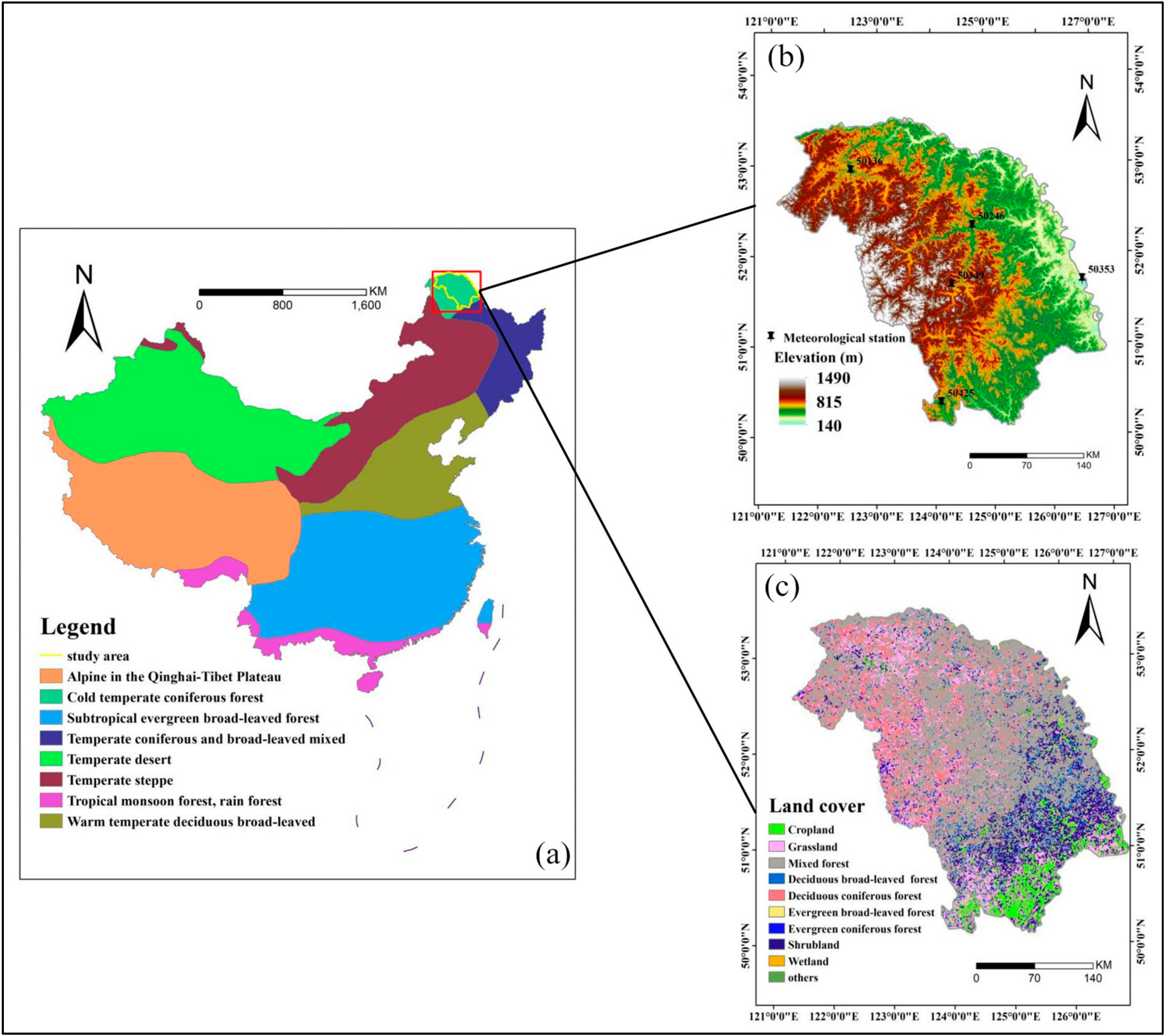
As shown in Figure 1a, the GKM region (50°10′~53°33′N, 121°12′~127°0′E) is located in the northernmost area of China. This study area is adjacent to the Lesser Khingan Mountains in the east, near the vast Hulunbeir Prairie in the west, bordering the fertile Songnen plain in the south, and separated from Siberia in Russia by the Heilongjiang River. Lying in the east slope of the Greater Khingan Mountains ridges (GKMR), the study area has an obvious decrease in elevation from southwest to northeast (Figure 1b). The GKM belongs to the frigid temperature monsoon climate zone, which has an annual average temperature of −2.6 °C. The annual average precipitation is 400–600 mm, and the majority of the precipitation is concentrated in July to September, providing a relatively humid environment for vegetation growing. The soils are mainly dark brown coniferous forest soils. The GKM is an important state-owned natural forest region that serves as a biological protective screen for northeastern and northern China. Also, it includes a first-grade National Nature Ecological Reserve with abundant forest resources whose area covers about 80% of this region (Figure 1c), including the largest and best preserved primeval cold-temperature bright coniferous forest in China (Figure 1a). However, its forest structure is relatively simple due to the cold weather. The dominant species are Larix gmelinii and Mongolian pine [45].
2.2. Data
2.2.1. GLASS GPP Dataset
GPP data was provided by the Global Land Surface Satellite (GLASS) program [48]. This GLASS-GPP product was estimated by an improved EC-LUE model, which was derived from only four variables: normalized different vegetation index (NDVI), photosynthetically active radiation (PAR), air temperature, and the Bowen ratio of sensible-to-latent heat flux. Given the invariant parameters (i.e., the potential LUE and optimal plant growth temperature) across the various land cover types [33], GPP can address the spatial and temporal dynamics of the carbon cycle. When compared with the MODIS-GPP product, the GLASS-GPP product exhibited a longer temporal cover, which includes data every eight days starting from 1982 to the present. Also, it can provide information of vegetation before and after 1987, when a disastrous fire occurred in the northern part of the GKM. In conclusion, the GLASS-GPP product demonstrated a high reliability with the revised EC-LUE model and had a long time series dataset [33], so it can be used to analyze the spatiotemporal distribution and variation of GPP in the GKM.
A total of 1564 scenes from 1982 to 2015 with 46 scenes per year were analyzed. The original eight-day GPP product exhibited a spatial resolution of 0.05° with WGS1984 coordinate. We extracted the GPP data using the GKM’s boundary and then projected the data to UTM. The Savitzky–Golay (S-G) filter [49] in the software TIMESAT [50] was used to smooth some outliers caused by the environment noise and system error of sensor in the original GPP time series. The S-G filter is widely used because it can remodel the raw time series dataset to closely capture the sudden change in original values. After the repeating test, we used a 4 × 4 filter window to rebuild the GPP time series data that was required in the following step. We finally calculated the accumulated GPP (AG) over a certain period (i.e., total GPP during the growing season) within one year.
2.2.2. Datasets for Auxiliary Analysis
Meteorological data from five field observation stations in the GKM (Figure 1b) were available from China’s meteorological data web [51]. Several daily meteorological parameters, including sunshine duration, average temperature, maximum temperature, minimum temperature, and precipitation, were used from 1982 to 2015, and then daily parameters were aggregated to determine seasonal averages for spring (March–May), summer (June–August), autumn (September–November), winter (December–February), and the growing season (April–October). Furthermore, with the inverse distance weighting (IDW) interpolation method, we obtained spatially distributed meteorological data that has the same spatial resolution as the GLASS-GPP products.
Phenological parameters were acquired from the 8-km AVHRR NDVI-3g product with a 15-day interval from 1982 to 2015 that was produced by the Global Inventory Modeling and Mapping Studies (GIMMS) project [52]. The AVHRR NDVI-3g dataset was generated with a maximum value composite (MVC) per half-month and then corrected to minimize the influence of calibration loss, volcanic eruptions, and orbit drift [26]. To eliminate bare soil and sparsely vegetated pixels on the NDVI image, we excluded pixels with a mean NDVI < 0.05 in the growing season. Similarly, the S-G filter was used to smooth the original NDVI data. Finally, the dynamic threshold method [53] was used to obtain the phenological parameters, and the results were consistent with previous studies [45,54].
Similar to the GPP product, the Fraction of Photosynthetically Active Radiation (FPAR) dataset of GLASS was used. This kind of product was derived from leaf area index (LAI) via the LUT method [55] and had the same spatiotemporal resolution as the GPP product.
2.3. Methods
2.3.1. Unary Linear Regression
On the basis of filtered GPP time series, we used unary linear regression [56] to acquire the interannual variation characteristics of GPP in the GKM during 1982–2015 at both the regional and pixel scale. Here, we assumed time t as an independent variable and GPP as a dependent variable to establish the unary linear regression equation. The principal of unary linear regression can be generalized by the following equation:
where n is the length of the study period (year of monitoring interval); GPPj is the accumulated GPP of j year; and, θ is the regression slope (annual change ratio of accumulated GPP) acquired by the least square method. θ > 0 indicates that the accumulated GPP increased over n years and vice versa.
2.3.2. Pearson Correlation
Pearson correlation is considered a standard method to analyze the relationship between two variables. It can be expressed as follows:
where xi and yi (i = 1, 2, ……, n) are the time series for two variables; and are the multi-year average values of two variables; and, r is the correlation coefficient. r > 0 indicates a positive correlation between two variables, whereas r < 0 suggests a negative correlation. The absolute value of r can represent the closeness of two variables; the larger the r, the closer the two variables are and vice versa.
Several factors affect the distribution and variation of GPP in both temporal and spatial dimensions. Meteorological elements and phenological parameters are widely considered as influencing factors and verified in many regions [40,57,58,59]. Apart from meteorological and phenological factors, we also considered FPAR, representing the structure and the adaptive capacity of vegetation, as a factor. Pearson Correlation analysis was conducted between the above factors and GPP during the period of 1982–2015 at a pixel resolution to assess the influence of individual environment drivers on vegetation dynamics.
2.3.3. Standardized Multivariate Linear Regression (SMLR) Model
The SMLR model combined several driving factors to explain the dynamics of GPP. To separate the relative contribution of each driving factor, the fraction in variation partitioning of the multiple standardized regression was applied. The SMLR model is expressed as follows:
where GPP represents a time series of accumulated GPP in the growing season (AGG); EDi (i = 1, 2, ……, n; n is the total of driving factors) is a time series of a certain influencing factor covering the whole study period at the pixel scale, including daily sunshine duration in summer, daily average temperature in summer, daily precipitation in summer, growing season length (GSL), and FPAR; and are the multi-year mean values of AGG and influencing factors, respectively. δGPP and δED are standard deviations of AGG and influencing factors. Each time series was normalized by subtracting its mean value and then dividing it by its standard deviation. Thus, any unit change in each variable has the same statistical meaning and the effects of changes in different factors can be compared. β1, β2… βn are regression coefficients that represent the importance of each driving factors to the GPP. Factors with a large coefficient were assumed to contribute more to the variation in GPP, and the largest coefficient was identified as the dominant factor to GPP in our study area during the period of 1982–2015. Also, we used the Variance Inflation Factor (VIF) to examine the multicollinearity of our driving factors before conducting the SMLR model. Significant multicollinearity exists when the VIF ≥ 10. Each SMLR model and their coefficients were verified by the F-test and t-test, respectively.
3. Results
Given that the GPP was nearly zero during winter in the GKM, only the AG in spring, summer, autumn, and the growing season (GS) were considered for analysis.
3.1. Spatial Distribution of GPP
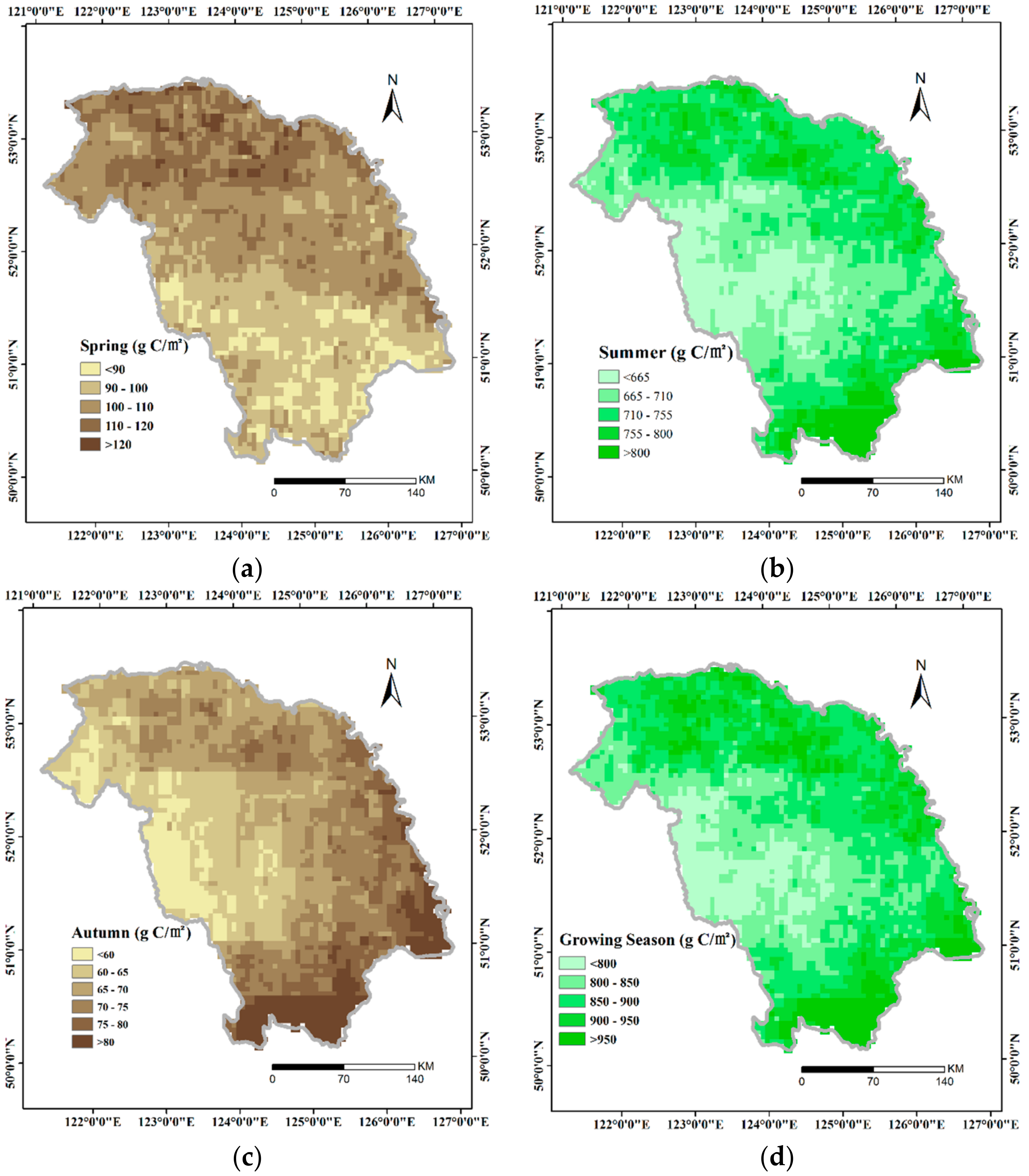
We acquired the multi-year mean AG in spring, summer, autumn, and the growing season to analyze the spatial distribution of GPP in the GKM over the past 34 years (1982–2015), and the results are shown in Figure 2. The spatial distribution of AG in the three seasons and the growing season differed considerably; in spring, the AG decreased from the northeast (134 g C/m2) to southwest (73 g C/m2). In summer, the northern extreme and southern extreme had large GPP values (>755 g C/m2), while the west central GKM had the smallest GPP values (<665 g C/m2). Different from spring and summer, high values began to concentrate in the southern GKM in autumn, whereas the middle part still had the lowest values. The spatial pattern of the AG during the growing season (AGG) showed great similarities to the AG in summer, but had larger spatial heterogeneity. The highest AGG value over the whole region reached 1070 g C/m2, and the lowest AGG value was about 680 g C/m2.
3.2. Changes in GPP at a Regional Scale
Temporal variation of GPP at the regional scale can be investigated from two perspectives: intra- and interannual variation.
Results in Figure 3 showed a significant annual unimodal variation in GPP across the GKM from 1982 to 2015. GPP values began to progressively increase in mid-April, rapidly rose during mid-May to late-June, and peaked in mid-July. In October, GPP values fell back to a relatively low level. June to August was the vigorous growth period with high GPP values in a year whose daily GPP was usually greater than 6 g C/m2.
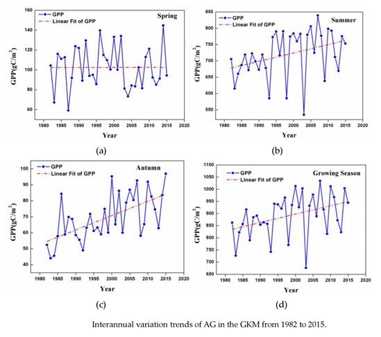
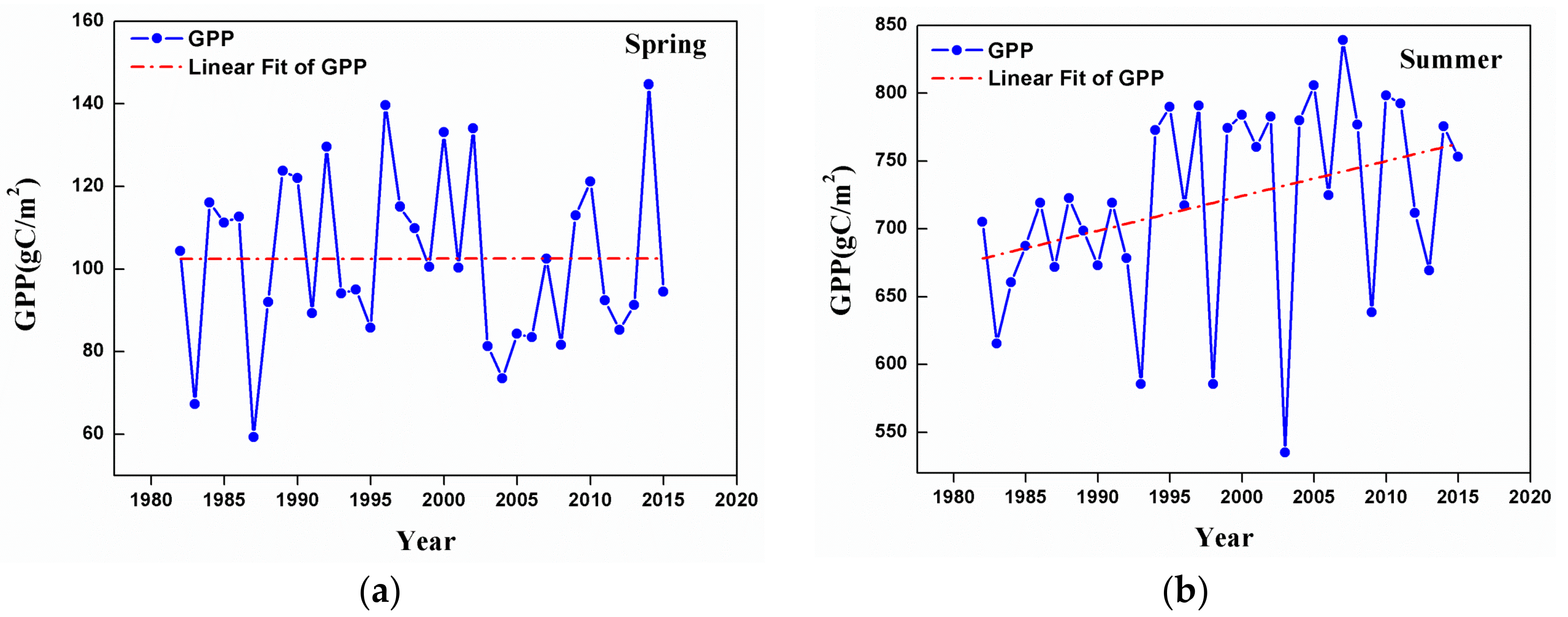
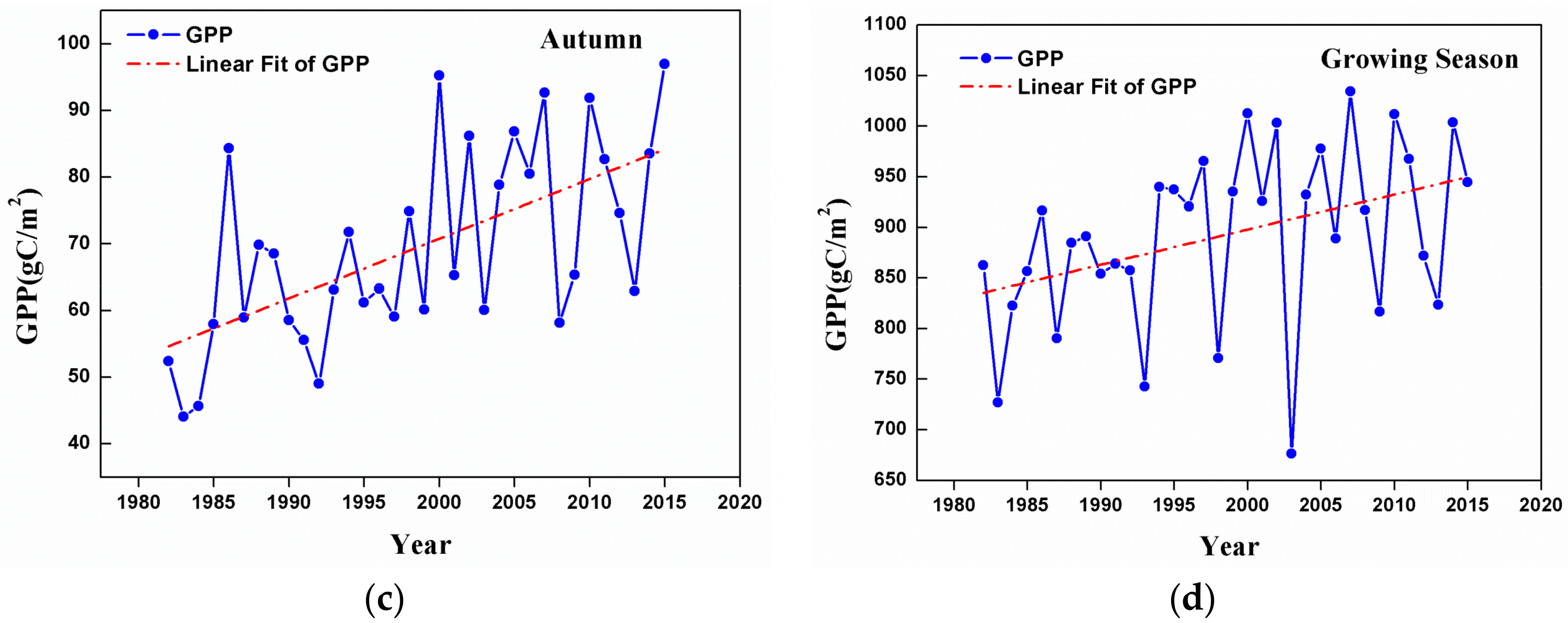
Apart from the spatial distribution of AG in different seasons, interannual AG trends in three seasons and the growing season in the GKM during 1982–2015 were calculated and are shown in Figure 4. Except for spring, the other two seasons and the growing season exhibited a significant increase in AG with fluctuations from 1982 to 2015 (Figure 4). However, the increasing levels varied. Among the three seasons, the AG in summer presented the biggest enhancement (ratio = 2.669 g C/m2 yr−1, p < 0.01), followed by the autumn (ratio = 0.89546 g C/m2 yr−1, p < 0.01). Statistics showed that the AG in summer accounted for 80% of the AGG of a year and thus could explain the majority increment in AGG.
In addition to the difference in variation trends, years with extreme AG values in different seasons also varied. In spring, the minimum AG occurred in 1987 and the maximum was in 2014. In summer, the minimum GPP occurred in 2003 and the maximum was in 2007; and, in autumn, the minimum and maximum AG occurred in 1982 and 2015, respectively. Also, extreme values in the growing season showed great similarities to those in summer.
3.3. Spatial Patterns of GPP Trend
Apart from interannual change at the regional scale, we also analyzed variation at the pixel scale. Because the AGG variation trend was not obvious before 1999, we only displayed linear trends of the AGG over progressively longer periods from 18 (1982–1999) to 34 (1982–2015) years, starting in 1982.
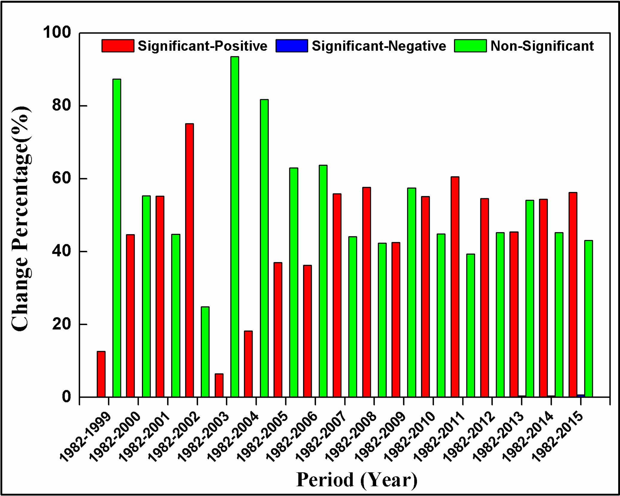
The amounts of pixels that are characterized by significantly increased AGG were greatly enhanced after 1999 (Figure 5). Two periods exhibited a notable increase: 1999–2002 and 2003–2008. A minor dip was observed in 2003 because of the combined effect of low temperature and adequate precipitation. After 2008, variations in the AGG became flat and the percentage of pixels with a significant increasing trend was maintained at about 57%.
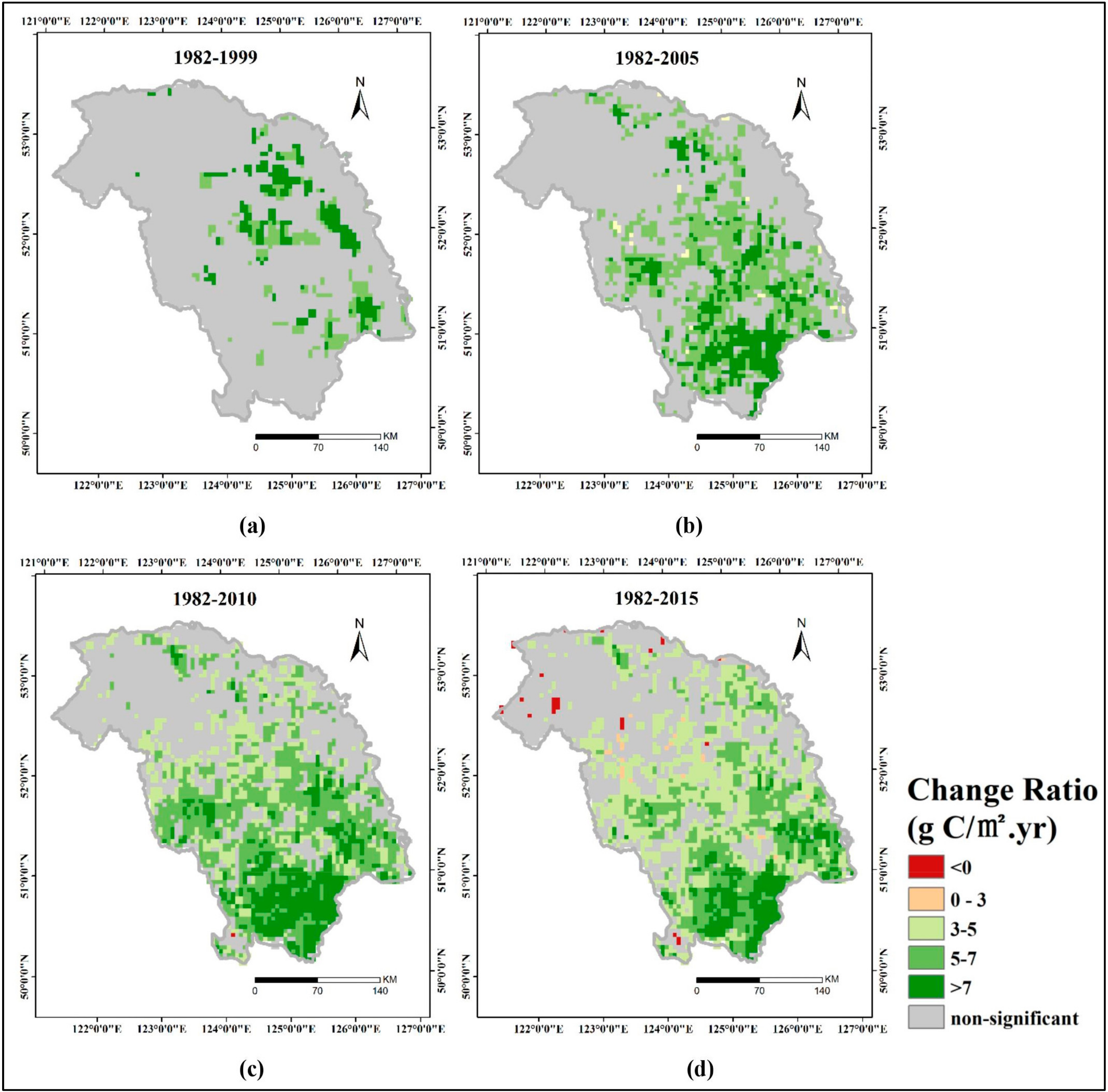
Further exploration (Figure 6) found that pixels characterized by significantly increased AGG mainly concentrated in the central and southern GKM, while most of the pixels in the north still showed non-significant trends during the study period. After 2010, though areas with increasing AGG were still expanding, the variation ratio of some areas, especially the middle part, decreased (comparing Figure 6c,d).
3.4. Correlations between GPP and Driving Factors
3.4.1. Effects of Local Meteorological Factors on GPP
In order to compare meteorological variables acquired from the meteorological stations with GPP values, the time series of GPP in the buffer distance of 25 km [60] around each meteorological station were extracted for 1982–2015. A Pearson correlation method was then performed between the extracted time-series and meteorological data to analyze the relationship between the GPP and meteorological factors. Because the effect of meteorological factors differed under varying seasons during the year, we calculated the correlation coefficient in different seasons, and the results are listed in Table 1.
In spring, sunshine duration and temperature played key roles in AG, while precipitation had little influence on AG during the study period. In summer, vegetation grew rapidly and AG was high. All of the factors had significant impacts on AG. Sunshine duration and temperature showed nearly the same positive effects on AG, while precipitation was negatively correlated with AG. AG in autumn and summer were alike in correlation with meteorological factors, but the effect of precipitation exceeded that of temperature in autumn and demonstrated an equally significant influence on AG as sunshine duration. As for AG in the growing season, the relationship between the AG and meteorological factors were basically the same as that in summer.
3.4.2. Effects of Phenological Parameters and FPAR on GPP
Based on the phenological parameters acquired as shown in Figure 7, we explored the relationship between the phenological parameters and GPP.
In the GKM, an advance in SOG and delay in EOG leaded to an obvious extension of GSL over the last 34 years. This result was consistent with previous findings, demonstrating that climate warming causes an extension of GSL [46,61].
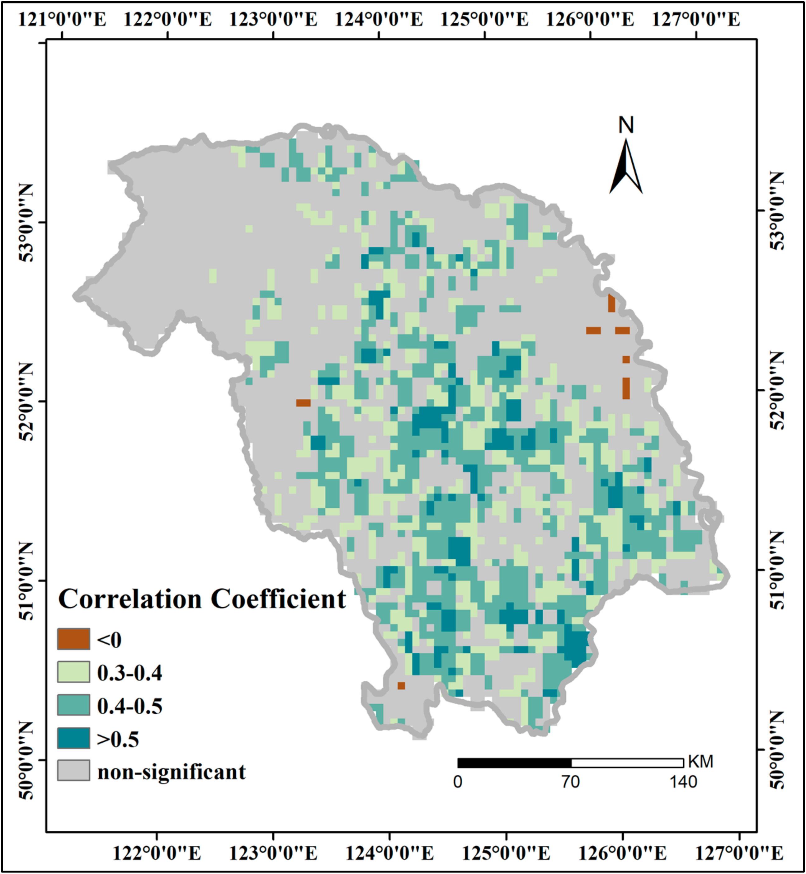
According to many studies [59,62,63] that were conducted in other regions, the extension of GSL is an important factor for the increasing GPP. We also conducted correlation analysis between GPP and GSL per pixel along the temporal dimension and obtained the spatial distribution of the correlation coefficient; the result is displayed in Figure 8.
Results (Figure 8) showed that in the central and southern GKM, there was a significant positive correlation between GSL and AGG, as was the case in abovementioned areas. The extension of GSL could explain the increase of AGG in some areas belonging to the GKM over the past 34 years, and this was consistent with the results of a previous study [59]. The majority of regions in the north and along the GKMR did not show a significant correlation between AGG and GSL, therefore some other elements should be considered as driving factors in those areas.
Apart from phenological parameters, FPAR, which refers to the fraction of absorbed PAR in vegetation photosynthesis, may also be an important driving factor for GPP, because it can directly impact the total vegetation productivity during photosynthesis. Correlation analysis, as depicted in Figure 9, showed a significant positive correlation between GPP and FPAR in the Mohe County, along the GKMR, and in part of the southern GKM, meaning that FPAR in the areas mention above was an important factor for AGG; however, little significant correlation was found in the central GKM.
A comparison between Figure 8 and Figure 9 showed a great difference of driving factors in different regions. It is necessary to combine all of the factors mentioned above to explore the spatial distribution of the dominant factor affecting GPP across the GKM; this will help us to further understand the underlying mechanism of vegetation dynamics in our study area over the past 34 years.
3.4.3. Dominant Factor for GPP Variation
The above-mentioned five factors (daily sunshine duration of summer, daily mean temperature of summer, daily precipitation of summer, GSL, and FPAR) all had a direct or indirect impact on GPP. In this section, we determined the regression between AGG and these five factors with an SMLR model at the pixel level, and thus found the dominant factor for the GPP variation.
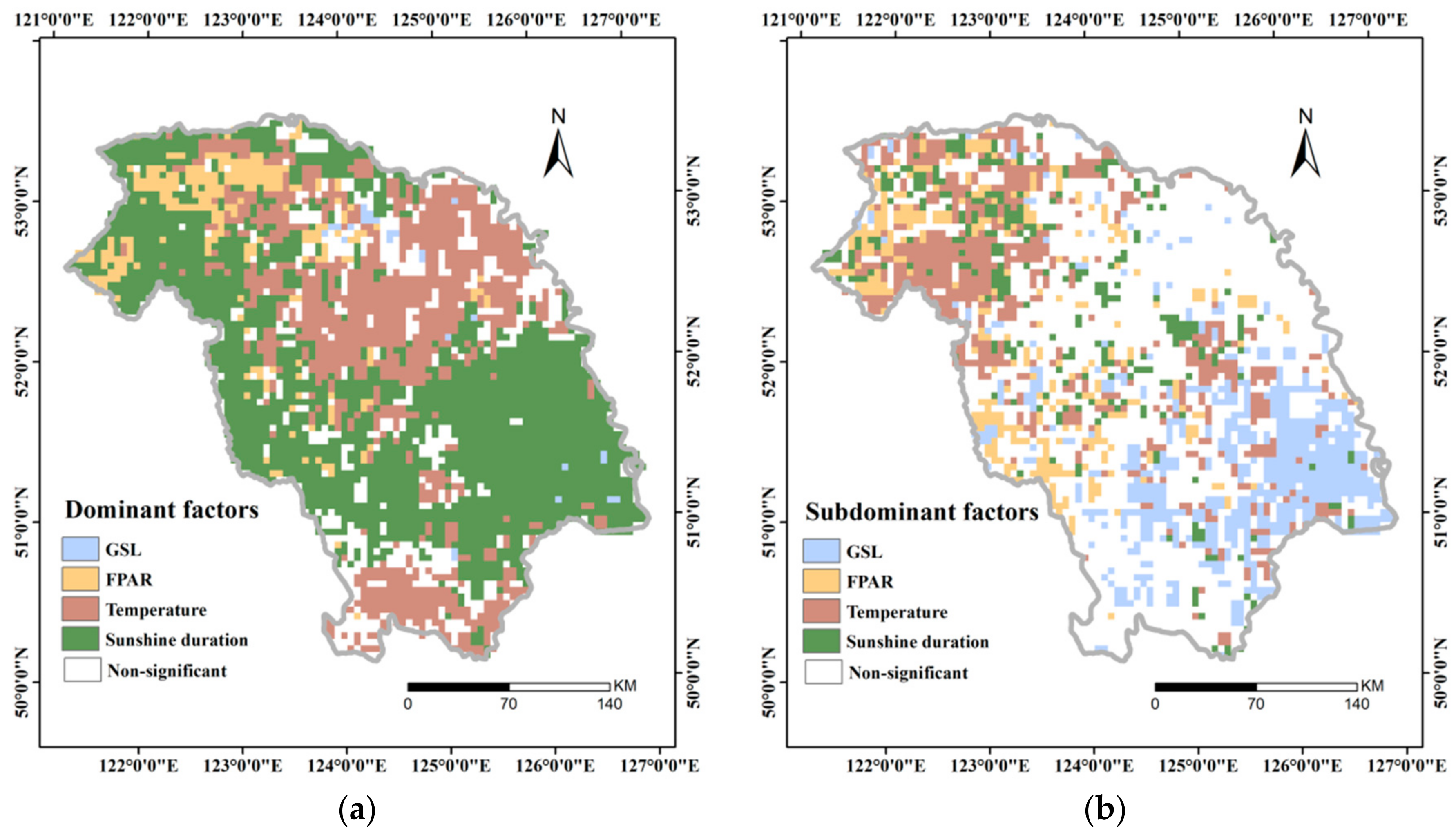
The result of the regression was displayed in Figure 10. It showed that, except for some areas in the northern GKM, most parts of the GKM were highly correlated with daily sunshine duration and mean temperature in summer, so these two factors acted as dominant or subdominant factors in our study area. Observations in an area called Mohe County in the northern GKM differed where most parts were closely related to FPAR instead of daily sunshine duration and mean temperature of summer. Furthermore, GSL and daily precipitation did not exert key effects on GPP when compared with the other three factors.
According to the coefficients before each independent variable derived from the SMLR model at the pixel level, we calculated the zonal mean value of coefficients for each dominant factor and the results are shown in Table 2. Taking sunshine duration as an example, when sunshine duration is a dominant factor in our study area, each unit increase in sunshine duration causes a 0.519 unit increase in AGG.
4. Discussions
4.1. Analysis of GPP Spatiotemporal Dynamics
In the GKM, different seasons displayed different patterns of spatial distribution and we considered three reasons for these phenomena according to our analysis. Understory vegetation, such as dwarf shrubs, mosses, and reindeer lichens, played an important role. Studies found that the productivity of understory vegetation is probably comparable with that of the trees [64], and this is especially obvious in spring when understory vegetation grew more lushly, while most of the trees were just starting to sprout new leaves, providing a bright environment in which understory vegetation can acquire more sunshine. The northern GKM had the largest AG values (Figure 2a) in spring, which can be attributed to understory vegetation. We found much evidence demonstrating that understory vegetation in the northern GKM was much lusher than that in other parts of the GKM. On one hand, a majority of bright coniferous forest, which is usually sparser than mixed broadleaf-conifer forest or broadleaf forest, mainly concentrated in the northern GKM (Figure 11 shows the contrast of spring AG in the bright coniferous zone and other areas), so understory vegetation flourished here [65]. On the other hand, fire is also a primary determinant for understory vegetation [64,66], so the disastrous fire that occurred in the northern GKM in 1987 may have contributed to the luxuriance of the understory vegetation in that region.
Altitude was another crucial factor for the spatial distribution of AG in our study area. GPP in areas lying along the Greater Khingan Mountain Ridges (GKMR) was always smaller than that in other parts (Figure 12 shows the variation of AGG with elevation, ratio = −0.18 g C/m2 m−1, p < 0.05); this was especially obvious in summer (as shown in Figure 3b). As we all know, temperature decreases with the increase in elevation, so the GKMR is a low-temperature zone with low GPP values by nature. In summer, vegetation in the high-temperature zone grew rapidly, while growth remained slow along the GKMR, so the gap in productivity increased further.
Land cover also influenced the spatial distribution of AG. When combining with land cover data of the GKM (Figure 1c), we found cropland, instead of forest, being widely distributed in the southern GKM (Figure 11 shows the contrast of spring AG in the cropland zone and other areas). Because of human intervention, cropland can grow well in a relatively low temperature and thus the southern GKM had the largest GPP values across the GKM in autumn when the temperature has greatly decreased.
Apart from spatial distribution, reasons for the temporal variation of AG were also analyzed. Annual variation in GPP displayed an obviously unimodal seasonal cycle because Larix gmelinii, a kind of deciduous coniferous forest, is the dominant species in the GKM. Due to the low temperature and frozen soil before the 100th day (mid-April) and after the 270th day (early-October), photosynthesis is weak and thus GPP is mainly produced from mid-May to mid-September, so there is a shorter growing period than in other regions.
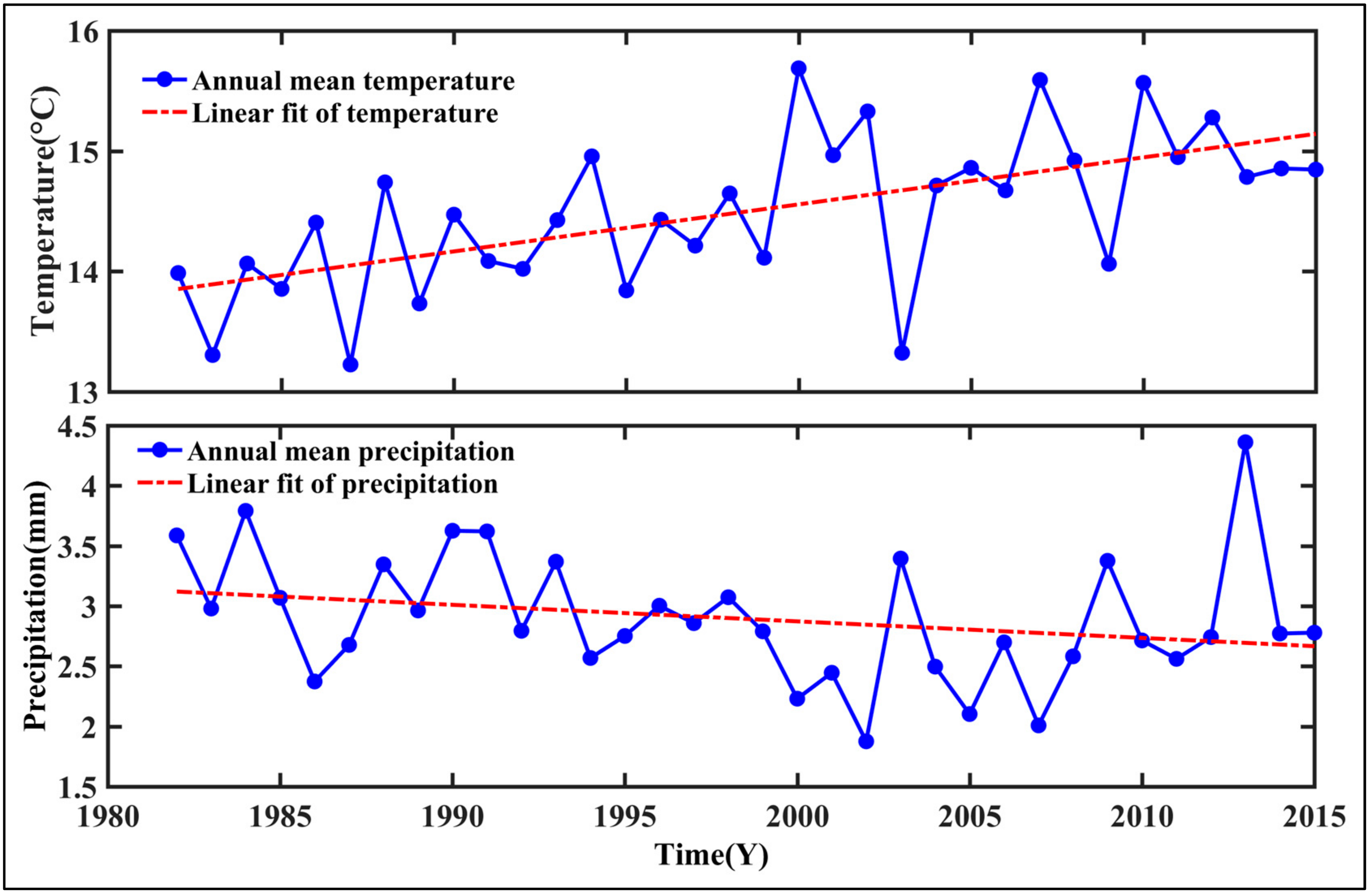
The interannual change of AG at the regional scale displayed significant increasing trends in summer, autumn, and the growing season; this observation was consistent with findings in a previous study [67]. Moreover, according to Figure 13 and previous studies [68,69], there was a significant warming and drying trend of the climate (daily average temperature: ratio = 0.0391 °C/yr−1, p < 0.01; daily precipitation: ratio = −0.0138 mm/yr−1, p = 0.146) in the GKM. What is more, our study area aggregates a number of heliophilous larch, which is suited to warm and dry environments, so the climate in the GKM benefitted vegetation growth and resulted in an obvious increase in the AG over the past 34 years.
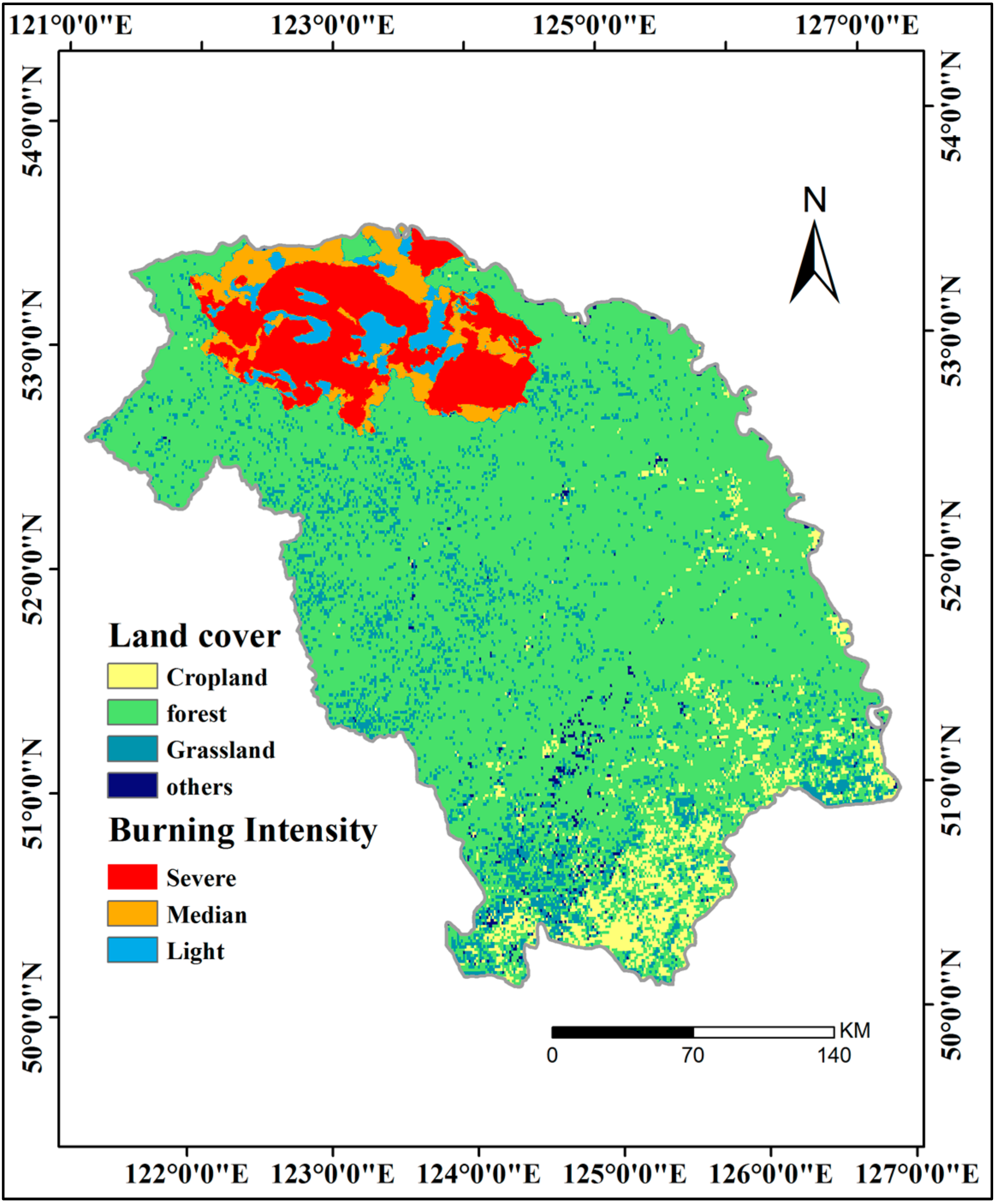
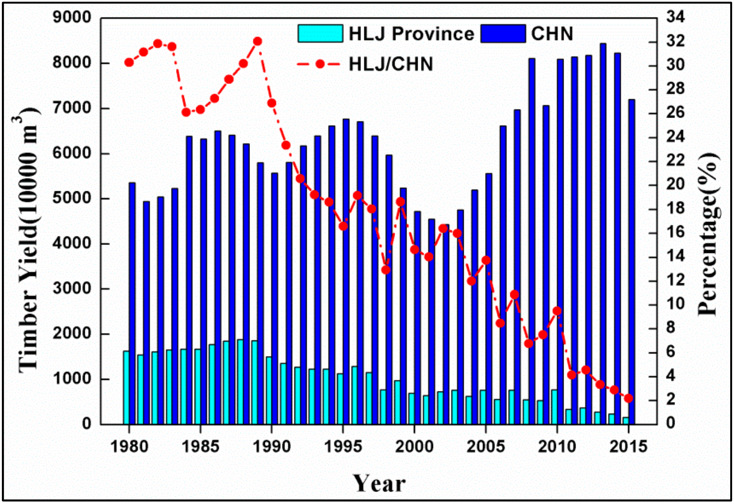
Further studies on interannual variation trends at the pixel scale did not find significant variation during 1982–1999. As an important source of commercial timbers in China, the effects of the GKM on maintaining ecological balance and improving the ecological environment have always been overlooked; for instance, intense anthropogenic activity intervention, such as reclamation and excessive deforestation, occurred frequently, which led to a dramatic drop in its forest areas. After the natural forest protection project launched in 1998, timber yield dramatically decreased (Figure 14). So, there was an obvious increment of AGG in the central and southern GKM entering the 21st century. Furthermore, the variation of AGG after 2010 was slowed down because of the formation of a relatively stable vegetation community in the GKM a decade after the natural forest protection project in 1998. Nevertheless, some regions in the northern GKM still showed little variation trend, which could partly be explained by the severe fire in 1987 (Figure 15). In severely burnt area, there was nearly no natural forestry resources left. A secondary succession procedure occurred, which had dynamic land cover [70,71,72,73] and led to the non-significant changing ratio of AGG.
4.2. The Response of GPP to Driving Factors
Daily sunshine duration in summer acted as a dominant factor for most regions in the GKM. The sunshine duration in meteorological observation is defined as the period during which direct solar irradiance exceeds a threshold value of 120 W/m² [74]. It is a general indicator of the cloudiness of a location [75]. According to Figure 13, a warming and drying trend has occurred in the GKM, so daily sunshine duration increased simultaneously. When compared with the impact of GSL on AGG by extending photosynthesis time in spring (advance of SOG) and autumn (delay of EOG), the daily sunshine duration in summer prolonged the photosynthesis time in summer when photosynthesis efficiency is high, and a slight extension of daily sunshine duration contributed to a large enhancement in AGG. Also, vegetation can absorb more solar radiation over a long sunshine duration, which is directly related to photosynthesis and was confirmed to be a limited factor in high latitude regions [76].
Temperature had positive effects on GPP, while precipitation had negative effects on GPP, which were in agreement with relevant study results [40,59,60,61]. GKM vegetation system was strongly constrained by low temperature, so the warming trend that is reported above was bound to increase GPP. Precipitation inhibited GPP across the GKM in most periods when precipitation was adequate, illumination time and temperature decreased with the thick cloud cover that was brought by precipitation, which weakened photosynthesis and reduced vegetation GPP; thus, the precipitation was not a direct factor for GPP. However, in spring when precipitation was rare, no obvious correlation between GPP and precipitation was found, due to the alimentation of snow.
FPAR, instead of sunshine duration and temperature, was a dominant factor in part of northern GKM. Overlay analysis revealed a high correlation of the above-mentioned areas with the severely burnt zone caused by the fire in 1987 (Figure 15). Previous studies [63,64,65] demonstrated a secondary succession process in burnt areas. Variation in vegetation type and tree age during the succession process may have contributed to a non-significant correlation between climate changes and GPP interannual variation in the northern GKM. On the other hand, FPAR is an important parameter for photosynthesis, and one previous study [77] revealed a close relationship between FPAR and vegetation type. Therefore, GPP in the severely burnt area in the northern GKM was closely related with FPAR.
4.3. Study Limitations
When compared with previous studies that used MODIS datasets after 2000 to analyze vegetation variation [78,79], this study used the GLASS GPP product and revealed the spatiotemporal characteristics of GPP in the GKM from 1982 to 2015. Obviously, an extension of the study period could provide much more information about the dynamic change of vegetation and the carbon cycle. However, some problems still existed. The precision of the GLASS-GPP time series in our study area needs to be verified with data observed in the eddy covariance flux tower, however, because of poor management, data acquired from the tower cannot be used in the verification, so supplementary analysis using the mainstream MODIS dataset is necessary for making a comparison. On the other hand, when compared with the distribution area of boreal forest (especially the bright coniferous forest), the spatial resolution of GLASS-GPP data that we used is a little coarser, and therefore details may be overlooked. For this reason, further studies combining with spatially finer TM datasets have been undertaken.
Uncertainty in our correlation results may be caused by the interpolated meteorological data, the calculated phenology parameters and pixel mismatches (use of remotely sensed data from different sources). The meteorological observation station are sparsely distributed in the GKM which is the northernmost part of China, there are only five stations in our study area and the remaining stations that are distributed around the GKM are far away. Moreover, there are no stations in the surrounding northern and eastern direction. All of these factors may increase the uncertainty of the interpolation. There are also some limitations that are caused by the phenological parameters. Although the phenology parameters we used have been verified by many relative studies [54,80], field observation data is still necessary for authenticity verification. Unfortunately, no field observation data is available for the GKM in the study period, so our work should be improved by further field observations. Pixel mismatches also caused some errors. Since we used remotely sensed data from different source, pixel mismatches were inevitable. For example, GLASS-GPP had a 5-km resolution, while NDVI had an 8-km resolution, so we resampled NDVI to match GPP data, which caused error in NDVI.
This paper only considered five factors affecting the spatiotemporal dynamics of GPP; other factors are also important, especially anthropogenic activities and fire in the GKM. For example, the natural forest protection project launched in 1998 played an important role in our study area, as mentioned above. However, because such roles hard to quantify, it is difficult for us to know their specific effect on GPP. What is more, we cannot entirely separate the effect that is brought by anthropogenic activities and the quantified environment factors, which added some uncertainty to our study. Therefore, further studies should be concentrated on finding alternatives and analyzing effects brought by anthropogenic activities and fire. Further study is needed before we can thoroughly understand the potential mechanisms affecting the spatiotemporal pattern of GPP in the GKM.
5. Conclusions
Based on an analysis of vegetation spatiotemporal dynamics as well as the correlation between GPP and its driving factors, we drew the following conclusions:
- In the GKM, different seasons displayed different patterns of spatial distribution because of the difference in understory vegetation, altitude and land cover. Areas with bright conifer forest always have a larger GPP because the understory vegetation contributes a great deal to vegetation total productivities. Altitude impacts GPP by changing temperature. Land cover with intense human intervention showed different seasonal changes in AGG.
- Temporal trends of AG at the regional scale showed a dramatic increase from 1982 to 2015 in summer, autumn, and the growing season. This observation could be considered to be a result of the warming and drying trend that is seen in the GKM over the past 34 years.
- Interannual GPP trends at the pixel scale showed that the areas with significant AGG variation (mostly significant increasing trends) were strikingly expanded after 2000 because of the natural forest protection project launched in 1998, but the AGG variation displayed a flattened trend over the last five years due to the formation of a relatively stable vegetation community.
- Upon aggregating all of the above factors, daily sunshine duration in summer, instead of GSL, acted as the dominant factor in most of the areas, whereas daily mean temperature in summer was the dominant factor in a fraction of the GKM. FPAR also acted as the dominant factor in part of the northern GKM and was closely related to vegetation change that was caused by the fire in 1987.
Acknowledgments
This research was supported by the Major State Basic Research Development Program of China (2013CB733402), the National Natural Science Foundation of China (grant Nos. 41271346, 91425301). We appreciate the provision of GPP and FPAR products by GLASS Team.
Author Contributions
All authors contributed significantly to this manuscript. Specific contributions include data collection (Ling Hu, Wenjie Fan), data analyses (Ling Hu, Wenjie Fan), methodology (Ling Hu, Wenjie Fan), and manuscript preparation (Ling Hu, Wenjie Fan, Huazhong Ren, Suhong Liu, Yaokui Cui, Peng Zhao).
Conflicts of Interest
The authors declare no conflict of interest.
References
- Tans, P.P.; Fung, I.Y.; Takahashi, T. Observational constraints on the global atmospheric CO2 budget. Science 1990, 247, 1431–1438. [Google Scholar] [CrossRef] [PubMed]
- Schimel, D.S.; Braswell, B.H.; McKeown, R.; Ojima, D.S.; Parton, W.J.; Pulliam, W. Climate and nitrogen controls on the geography and timescales of terrestrial biogeochemical cycling. Glob. Biogeochem. Cycles 1996, 10, 677–692. [Google Scholar] [CrossRef]
- Zhou, L.M.; Tucker, C.J.; Kaufmann, R.K.; Slayback, D.; Shabanov, N.V.; Myneni, R.B. Variations in northern vegetation activity inferred from satellite data of vegetation index during 1981 to 1999. J. Geophys. Res. 2001, 106, 20069–20083. [Google Scholar] [CrossRef]
- Melillo, J.M.; Mcguire, A.D.; Kicklighter, D.W.; Moore, B.; Vorosmarty, C.J.; Schloss, A.L. Global climate-change and terrestrial net primary production. Nature 1993, 363, 234–240. [Google Scholar] [CrossRef]
- Fang, J.Y.; Chen, A.P.; Peng, C.H.; Zhao, S.Q.; Ci, L.J. Changes in forest biomass carbon storage in China between 1949 and 1998. Science 2001, 292, 2320–2322. [Google Scholar] [CrossRef] [PubMed]
- Xiao, X.M.; Hollinger, D.; Aber, J.; Goltz, M.; Davidson, E.A.; Zhang, Q.Y.; Moore, B. Satellite-based modeling of gross primary production in an evergreen needleleaf forest. Remote Sens. Environ. 2004, 89, 519–534. [Google Scholar] [CrossRef]
- Nemani, R.; Keeling, C.; Hashimoto, H.; Jolly, W.; Piper, S.; Tucker, C.; Myneni, R.; Running, S. Climate-driving increases in global terrestrial net primary production from 1982 to 1999. Science 2003, 300, 1560–1563. [Google Scholar] [CrossRef] [PubMed]
- Zhu, Z.C.; Piao, S.L.; Myneni, R.B.; Huang, M.T.; Zeng, Z.Z.; Canadell, J.G.; Ciais, P.; Sitch, S.; Friedlingstein, P.; Arneth, A.; et al. Greening of the Earth and its drivers. Nat. Clim. Chang. 2016, 6, 791–795. [Google Scholar] [CrossRef]
- Chapin, M.C.; Matson, P.A.; Mooney, H.A. Principles of Terrestrial Ecosystem Ecology, 2nd ed.; Spring: New York, NY, USA, 2002; p. 102. [Google Scholar]
- Beer, C.; Reichstein, M.; Tomelleri, E.; Ciais, P.; Jung, M.; Carvalhais, N.; Rodenbeck, C.; Arain, M.A.; Baldocchi, D.; Bonan, G.B.; et al. Terrestrial gross carbon dioxide uptake: Global distribution and covariation with climate. Science 2010, 329, 834–838. [Google Scholar] [CrossRef] [PubMed]
- Anav, A.; Friedlingstein, P.; Beer, C.; Ciais, P.; Harper, A.; Jones, C.; Murray-Tortarolo, G.; Papale, D.; Parazoo, N.C.; Peylin, P.; et al. Spatiotemporal patterns of terrestrial gross primary production: A review. Rev. Geophys. 2015, 53, 785–818. [Google Scholar] [CrossRef] [Green Version]
- Jensen, M.N. Consensus on ecological impacts remains elusive. Science 2003, 299, 38. [Google Scholar] [CrossRef] [PubMed]
- Cox, P.; Jones, C. Illuminating the modern dance of climate and CO2. Science 2008, 321, 1642–1644. [Google Scholar] [CrossRef] [PubMed]
- Battin, T.J.; Kaplan, L.A.; Findlay, S.; Hopkinson, C.S.; Marti, E.; Packman, A.I.; Newbold, J.D.; Sabater, F. The boundless carbon cycle. Nat. Geosci. 2009, 2, 598–600. [Google Scholar] [CrossRef]
- NASA. Earth System Science: A Closer View; NASA: Washington, DC, USA, 1988; p. 208. [Google Scholar]
- Myneni, R.; Hoffman, R.; Knyazikhin, Y.; Privette, J.; Glassy, J.; Tian, H. Global products of vegetation leaf area and fraction absorbed PAR from one year of MODIS data. Remote Sens. Environ. 2002, 83, 214–231. [Google Scholar] [CrossRef]
- Gutman, G.; Ignatov, A. Global land monitoring from AVHRR: Potential and limitations. Int. J. Remote Sens. 1995, 16, 2301–2309. [Google Scholar] [CrossRef]
- Privette, J.L.; Fowler, C.; Wick, G.A.; Baldwin, D.; Emery, W.J. Effect of orbital drift on advanced very high resolution radiometer products Normalized difference vegetation index and sea surface temperature. Remote Sens. Environ. 1995, 53, 164–17l. [Google Scholar] [CrossRef]
- Rao, C.R.N.; Chen, J. Inter-satellite calibration linkages for the visible and near-infrared channels of the Advanced Very High Resolution Radiometer on the NOAA-7,-9, and-11 spacecraft. Int. J. Remote Sens. 1995, 16, 1931–1942. [Google Scholar]
- Rao, C.R.N.; Chen, J. Post-launch calibration of the visible and near-infrared channels of the Advanced Very High Resolution Radiometer (AVHRR) on the NOAA-14 spacecraft. Int. J. Remote Sens. 1996, 17, 2743–2747. [Google Scholar] [CrossRef]
- Myneni, R.B.; Tucker, C.J.; Asrar, G.; Keeling, C.D. Interannual variations in satellite-sensed vegetation index data from 1981 to 1991. J. Geophys. Res. 1998, 103, 6145–6160. [Google Scholar] [CrossRef]
- Gutman, G.G. On the use of long-term global data of land reflectances and vegetation indices derived from the advanced very high resolution radiometer. J. Geophys. Res. 1999, 104, 6241–6255. [Google Scholar] [CrossRef]
- Monteith, J.L. Solar radiation and productivity in tropical ecosystems. J. Appl. Ecol. 1972, 9, 747–766. [Google Scholar] [CrossRef]
- Monteith, J.L. Climate and the efficiency of crop production in Britain. Phil. Trans. R. Soc. B. 1977, 281, 277–294. [Google Scholar] [CrossRef]
- Goetz, S.J.; Prince, S.D. Modelling terrestrial carbon exchange and storage: Evidence and implications of functional convergence in light-use efficien Cycles. Adv. Ecol. Res. 1999, 28, 57–92. [Google Scholar]
- Tucker, C.J.; Pinzon, J.E.; Brown, M.E.; Slayback, D.A.; Pak, E.W.; Mahoney, R.; Vermote, E.F.; Saleous, N.E. An extended AVHRR 8-km NDVI dataset compatible with MODIS and SPOT vegetation NDVI data. Int. J. Remote Sens. 2005, 26, 4485–4498. [Google Scholar] [CrossRef]
- Hilker, T.; Coops, N.C.; Hall, F.G.; Black, T.A.; Wulder, M.A.; Nesic, Z.; Krishnan, P. Separating physiologically and directionally induced changes in PRI using BRDF models. Rem. Sens. Environ. 2008, 112, 2777–2788. [Google Scholar] [CrossRef]
- Prince, S.D.; Goward, S.N. Global net primary production: A remote sensing approach. J. Biogeogr. 1995, 22, 815–835. [Google Scholar] [CrossRef]
- Wei, S.H.; Yi, C.X.; Fang, W.; Hendrey, G. A global study of GPP focusing on light-use efficiency in a random forest regression model. Ecosphere 2017, 8, e01724. [Google Scholar] [CrossRef]
- Potter, C.S.; Randers, J.T.; Field, C.B.; Matson, P.A.; Vitousek, P.M.; Mooney, H.A.; Klooster, S.A. Terrestrial ecosystem production: A process model based on global satellite and surface data. Glob. Biogeochem. Cycles 1993, 7, 811–841. [Google Scholar] [CrossRef]
- Field, C.B.; Randerson, J.T.; Malmström, C.M. Global net primary production: Combining ecology and remote sensing. Remote Sens. Environ. 1995, 51, 74–88. [Google Scholar] [CrossRef]
- Yuan, W.P.; Liu, S.G.; Zhou, G.S.; Zhou, G.Y.; Tieszen, L.L.; Baldocchi, D.; Bernhofer, C.; Gholz, H.; Goldstein, A.H.; Goulden, M.L.; et al. Deriving a light use efficiency model from eddy covariance flux data for predicting daily gross primary production across biomes. Agric. For. Meteorol. 2007, 143, 189–207. [Google Scholar] [CrossRef]
- Yuan, W.P.; Liu, S.G.; Yu, G.R.; Bonnefond, J.M.; Chen, J.Q.; Davis, K.; Desai, A.R.; Goldstein, A.H.; Gianelle, D.; Rossi, F.; et al. Global estimates of evapotranspiration and gross primary production based on MODIS and global meteorology data. Remote Sens. Environ. 2010, 114, 1416–1431. [Google Scholar] [CrossRef]
- Veroustraete, F.; Sabbe, H.; Eerens, H. Estimation of carbon mass fluxes over Europe using the C-Fix model and Euroflux data. Remote Sens. Environ. 2002, 83, 376–399. [Google Scholar] [CrossRef]
- Running, S.W.; Nemani, R.R.; Heinsch, F.A.; Zhao, M.S.; Reeves, M.; Hashimoto, H. A continuous satellite-derived measure of global terrestrial primary production. Bioscience 2004, 54, 547–560. [Google Scholar] [CrossRef]
- Xiao, X.M.; Zhang, Q.Y.; Braswell, B.; Urbanski, S.; Boles, S.; Wofsy, S.; Moore, B., III; Ojima, D. Modeling gross primary production of temperate deciduous broadleaf forest using satellite images and climate data. Remote Sens. Environ. 2004, 91, 256–270. [Google Scholar] [CrossRef]
- Turner, D.P.; Ritts, W.D.; Styles, J.M.; Yang, Z.; Cohen, W.B.; Law, B.E.; Thornton, P.E. A diagnostic carbon flux model to monitor the effects of disturbance and interannual variation in climate on regional NEP. Tellus B 2006, 58, 476–490. [Google Scholar] [CrossRef]
- King, D.A.; Turner, D.P.; Ritts, W.D. Parameterization of a diagnostic carbon cycle model for continental scale application. Remote Sens. Environ. 2011, 115, 1653–1664. [Google Scholar] [CrossRef]
- Yao, Y.T.; Wang, X.H.; Li, Y.; Wang, T.; Shen, M.G.; Du, M.Y.; He, H.L.; Li, Y.; Luo, W.; Ma, M.; et al. Spatiotemporal pattern of gross primary productivity and its covariation with climate in China over the last thirty years. Glob. Change Biol. 2017, 24, 184–196. [Google Scholar] [CrossRef] [PubMed]
- Zscheischler, J.; Mahecha, M.D.; Buttlar, J.; Harmeling, S.; Jung, M.; Rammig, A.; Randerson, J.T.; Schölkopf, B.; Seneviratne, S.; Tomelleri, E.; et al. A few extreme events dominate global interannual variability in gross primary production. Environ. Res. Lett. 2014, 9, 035001. [Google Scholar] [CrossRef]
- Churkina, G.; Running, S.W. Contrasting climatic controls on the estimated productivity of global terrestrial biomes. Ecosystems 1998, 1, 206–215. [Google Scholar] [CrossRef]
- Piao, S.L.; Ciais, P.; Friedlingstein, P.; Noblet-Ducoudré, N.; Cadule, P.; Viovy, N.; Wang, T. Spatiotemporal patterns of terrestrial carbon cycle during the 20th century. Glob. Biogeochem. Cycles 2009, 23, GB4026. [Google Scholar] [CrossRef]
- Goulden, M.L.; Munger, J.W.; Fan, S.M.; Daube, B.C.; Wofsy, S.C. Exchange of carbon dioxide by a deciduous forest: Response to interannual climate variability. Science 1996, 271, 1576–1578. [Google Scholar] [CrossRef]
- Fang, J.Y.; Chen, A.P. Dynamic forest biomass carbon pools in China and their significance. Acta Bot. Sin. 2001, 43, 967–973. [Google Scholar]
- Zhao, H.Y.; Gong, L.J.; Qu, H.H.; Zhu, H.X.; Li, X.F.; Zhao, F. The climate change variations in the northern Greater Khingan Mountains during the past centuries. J. Geogr. Sci. 2016, 26, 585–602. [Google Scholar] [CrossRef]
- Cai, H.Y.; Zhang, S.W.; Yang, X.H. Forest Dynamics and Their Phenological Response to Climate Warming in the Khingan Mountains, Northeastern China. Int. J. Environ. Res. Pub. Health 2012, 9, 3943–3953. [Google Scholar] [CrossRef] [PubMed]
- Editorial Board of Vegetation Map of China. Chinese Academy of Science. In Vegetation Atlas of China (1:1,000,000); Geological Publishing House: Beijing, China, 2007. [Google Scholar]
- Global Land Surface Satellite (GLASS) Products Download and Service. Available online: http://glass-product.bnu.edu.cn/ (accessed on 1 December 2016).
- Savitzky, A.; Golay, M. Smoothing and differentiation of data by simplified least squares procedures. Anal. Chem. 1964, 36, 1627–1638. [Google Scholar] [CrossRef]
- Eklundh, L.; Jonsson, P. TIMESAT 3.0 Software Manual; Malmö University: Malmö, Sweden, 2010. [Google Scholar]
- Chinese Meteorological Data Service Center (CMDC). Available online: http://data.cma.cn/ (accessed on 1 October 2016).
- NASA Ames Ecological Forecasting Lab. Available online: https://ecocast.arc.nasa.gov/data/pub/gimms/3g.v1/ (accessed on 20 December 2016).
- You, X.Z.; Meng, J.H.; Zhang, M.; Dong, T.F. Remote Sensing Based Detection of Crop Phenology for Agricultural Zones in China Using a New Threshold Method. Remote Sens. 2013, 5, 3190–3211. [Google Scholar] [CrossRef]
- Zhao, J.J.; Wang, Y.Y.; Zhang, Z.X.; Zhang, H.Y.; Hong, Y.; Guo, X.Y.; Yu, S.; Du, W.L.; Huang, F. The Variations of Land Surface Phenology in Northeast China and Its Responses to Climate Change from 1982 to 2013. Remote Sens. 2016, 8, 400. [Google Scholar] [CrossRef]
- Xiao, Z.Q.; Liang, S.L.; Sun, R.; Wang, J.D.; Jiang, B. Estimating the fraction of absorbed photosynthetically active radiation from the MODIS data based GLASS leaf area index product. Remote Sens. Environ. 2015, 171, 105–117. [Google Scholar] [CrossRef]
- Huang, K.; Zhang, Y.J.; Zhu, J.T.; Liu, Y.J.; Zu, J.X.; Zhang, J. The Influences of Climate Change and Human Activities on Vegetation Dynamics in the Qinghai-Tibet Plateau. Remote Sens. 2016, 8, 876. [Google Scholar] [CrossRef]
- Weber, U.; Jung, M.; Reichstein, M.; Beer, C.; Braakhekke, M.C.; Lehsten, V.; Ghent, D.; Kaduk, J.; Viovy, N.; Ciais, P.; et al. The interannual variability of Africa's ecosystem productivity: A multi-model analysis. Biogeosciences 2009, 6, 285–295. [Google Scholar] [CrossRef]
- Peng, S.S.; Piao, S.L.; Ciais, P.; Myneni, R.B.; Chen, A.; Chevallier, F.; Dolman, A.J.; Janssens, I.A.; Peñuelas, J.; Zhang, G.X.; et al. Asymmetric effects of daytime and night-time warming on Northern Hemisphere vegetation. Nature 2013, 501, 88–92. [Google Scholar] [CrossRef] [PubMed]
- Zhao, M.; Running, S.W. Drought-induced reduction in global terrestrial net primary production from 2000 through 2009. Science 2010, 329, 940–943. [Google Scholar] [CrossRef] [PubMed]
- Davis, C.L.; Hoffman, M.T.; Roberts, W. Long-term trends in vegetation phenology and productivity over Namaqualand using the GIMMS AVHRR NDVI3g data from 1982 to 2011. S. Afr. J. Bot. 2017, 111, 76–85. [Google Scholar] [CrossRef]
- Tang, H.; Li, Z.W.; Zhu, Z.L.; Chen, B.; Zhang, B.H.; Xin, X.P. Variability and Climate Change Trend in Vegetation Phenology of Recent Decades in the Greater Khingan Mountain Area, Northeastern China. Remote Sens. 2015, 7, 11914–11932. [Google Scholar] [CrossRef]
- Piao, S.L.; Friedlingstein, P.; Ciais, P.; Viovy, N.; Demarty, J. Growing season extension and its impact on terrestrial carbon cycle in the Northern Hemisphere over the past 2 decades. Global Biogeochem. Cycles 2007, 21, GB3018. [Google Scholar] [CrossRef]
- Murray-Tortarolo, G.; Anav, A.; Friedlingstein, P.; Sitch, S.; Piao, S.L.; Zhu, Z.; Poulter, B.; Zaehle, S.; Ahlström, A.; Lomas, M.; et al. Evaluation of land surface models in reproducing satellite-derived LAI over the high-latitude Northern Hemisphere. Part I: Uncoupled DGVMs. Remote Sens. 2013, 5, 4819–4838. [Google Scholar] [CrossRef] [Green Version]
- Nilsson, M.C.; Wardle, D.A. Understory vegetation as a forest ecosystem driver: Evidence from the northern Swedish boreal forest. Front Ecol. Environ. 2005, 3, 421–428. [Google Scholar] [CrossRef]
- Liu, Y.; Liu, R.G.; Pisek, J.; Chen, J.M. Separating overstory and understory leaf area indices for global needleleaf and deciduous broadleaf forests by fusion of MODIS and MISR data. Biogeosciences 2017, 14, 1093–1110. [Google Scholar] [CrossRef]
- Liu, Z.; Yang, J. Quantifying ecological drivers of ecosystem productivity of the early successional boreal Larix gmelinii forest. Ecosphere 2014, 5, 1–16. [Google Scholar] [CrossRef]
- Myneni, R.B.; Keeling, C.; Tucker, C.; Asrar, G.; Nemani, R. Increased plant growth in the northern high latitudes from 1981 to 1991. Nature 1997, 386, 698–702. [Google Scholar] [CrossRef]
- Zhang, Y.P.; Hu, H.Q. Climatic Change and Its Impact on Forest Fire in Daxing’ anling Mountains. J. North-East For. Univ. 2008, 36, 29–31. [Google Scholar]
- Gao, Y.G.; Zhao, H.Y.; Gao, F.; Zhu, H.X.; Qu, H.H.; Zhao, F. Climate change trend in future and its influence on wetlands in the Greater Khingan Mountains. J. Glaciol. Geocryol. 2016, 38, 47–56. [Google Scholar]
- Han, X.C.; Zhao, Y.S.; Xin, Y. Succession process of Larix gmelinii forest with artificial restoration after fire in Daxing’ anling. Sci. Soil Water Conserv. 2015, 13, 70–76. [Google Scholar]
- Rull, V. A palynological record of a secondary succession after fire in the Gran Sabana, Venezuela. J. Quat. Sci. 1999, 14, 137–152. [Google Scholar] [CrossRef]
- Wang, C.K.; Gower, S.T.; Wang, Y.H.; Zhao, H.X.; Yan, P.; Bond-Lamberty, B.P. The influence of fire on carbon distribution and net primary production of boreal Larix gmelinii forests in north-eastern China. Glob. Chang. Biol. 2001, 7, 719–730. [Google Scholar] [CrossRef]
- Wang, X.G.; Li, X.Z.; He, H.S.; Leng, W.F.; Wen, Q.C. Postfire succession of larch forest on the northern slope of Daxinganling. Chin. J. Ecol. 2004, 23, 35–41. [Google Scholar]
- Artz, R.; Ball, G.; Behrens, K.; Bonnin, G.M.; Bower, C.A.; Canterford, R.; Childs, B.; Claude, H.; Crum, T.; Dombrowsky, R.; et al. Measurement of Sunshine Duration. In Guide to Meteorological Instruments and Methods of Observation, 7th ed.; 7 bis, avenue de la Paix P.O. Box No. 2300 CH-1211 Geneva 2; WMO: Geneva, Switzerland, 2008; Volume 8, p. 199. ISBN 978-92-63-10008-5. [Google Scholar]
- Wikipedia. Available online: https://en.wikipedia.org/wiki/Sunshine_duration (accessed on 1 May 2017).
- Piao, S.L.; Nan, H.J.; Huntingford, C.; Ciais, P.; Friedlingstein, P.; Sitch, S.; Peng, S.S.; Ahlström, A.; Canadell, J.G.; Cong, N.; et al. Evidence for a weakening relationship between inter-annual temperature variability and northern vegetation activity. Nat. Commun. 2014, 5, 5018. [Google Scholar] [CrossRef] [PubMed] [Green Version]
- Peng, D.L.; Zhang, B.; Liu, L.Y.; Fang, H.L.; Chen, D.M.; Hu, Y.; Liu, L.L. Characteristics and drivers of global NDVI-based FPAR from 1982 to 2006. Global Biogeochem. Cycles 2012, 26, GB3015. [Google Scholar] [CrossRef]
- Karami, M.; Hansen, B.U.; Nielsen, A.W.; Abermann, J.; Lund, M.; Schmidt, N.M.; Elberling, B. Vegetation phenology gradients along the west and east coasts of Greenland from 2001 to 2015. Ambio 2017, 46 (Suppl. 1), S94–S105. [Google Scholar] [CrossRef] [PubMed]
- Qiu, B.W.; Zeng, C.Y.; Tang, Z.H.; Chen, C.C. Characterizing spatiotemporal non-stationarity in vegetation dynamics in China using MODIS EVI dataset. Environ. Monit. Assess. 2013, 185, 9019–9035. [Google Scholar] [CrossRef] [PubMed]
- Hou, X.H.; Niu, Z.; Gao, S. Phenology of Forest Vegetation in Northeast of China in Ten Years Using Remote Sensing. Spectrosc. Spectr. Anal. 2013, 34, 515–519. [Google Scholar]
Figure 1.
(a) Distribution of vegetation type and location of the Greater Khingan Mountains (GKM) in China, based on the Vegetation Regionalization Map of China (1:6,000,000) [47]; (b) DEM(Digital Elevation Model) and the meteorological station of the GKM; and, (c) Land cover of the GKM. The land cover data is from the MODIS dataset of 2001.

Figure 2.
Spatial distribution of (a) spring-average accumulated gross primary productivity (AG); (b) summer-average AG; (c) autumn-average AG; and, (d) growing season (GS)-average AG during 1982–2015.
Figure 2.
Spatial distribution of (a) spring-average accumulated gross primary productivity (AG); (b) summer-average AG; (c) autumn-average AG; and, (d) growing season (GS)-average AG during 1982–2015.

Figure 3.
Intra-annual variation characteristic of gross primary productivity (GPP) values during 1982–2015.
Figure 3.
Intra-annual variation characteristic of gross primary productivity (GPP) values during 1982–2015.
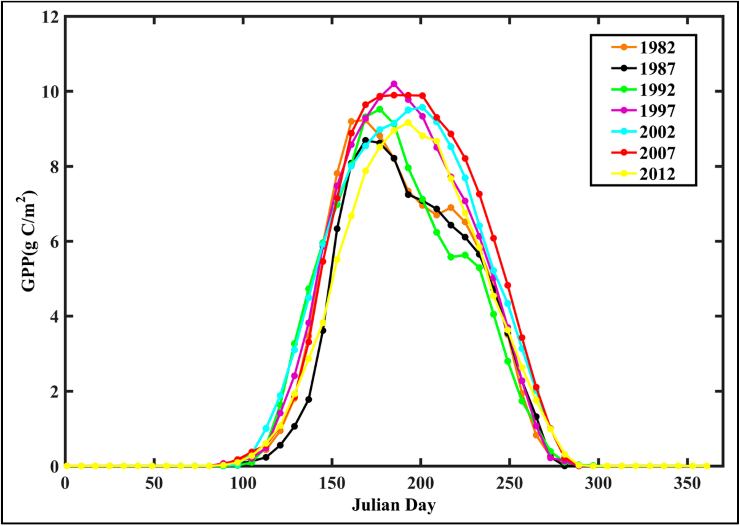
Figure 4.
Interannual variation trends of AG in the GKM from 1982 to 2015.


Figure 5.
Area fraction of the AGG displaying different statistical significance levels with progressively longer time series since 1982 (%). Significant positive stands for the increasing of GPP and significant negative refers to the reduction of GPP; both indicate a statistical significance of the linear regression with a Pearson correlation less than 0.05.

Figure 6.
Spatial distribution of AGG trends across the GKM during the periods of (a) 1982–1999; (b) 1982–2005; (c) 1982–2010; and, (d) 1982–2015. The linear trends of the AGG were calculated at the 95% confidence level.
Figure 6.
Spatial distribution of AGG trends across the GKM during the periods of (a) 1982–1999; (b) 1982–2005; (c) 1982–2010; and, (d) 1982–2015. The linear trends of the AGG were calculated at the 95% confidence level.

Figure 7.
Variation in phenological parameters in the GKM from 1982 to 2014 (SOG means starting day of growing season, EOG means ending day of growing season, and GSL means growing season length).
Figure 7.
Variation in phenological parameters in the GKM from 1982 to 2014 (SOG means starting day of growing season, EOG means ending day of growing season, and GSL means growing season length).
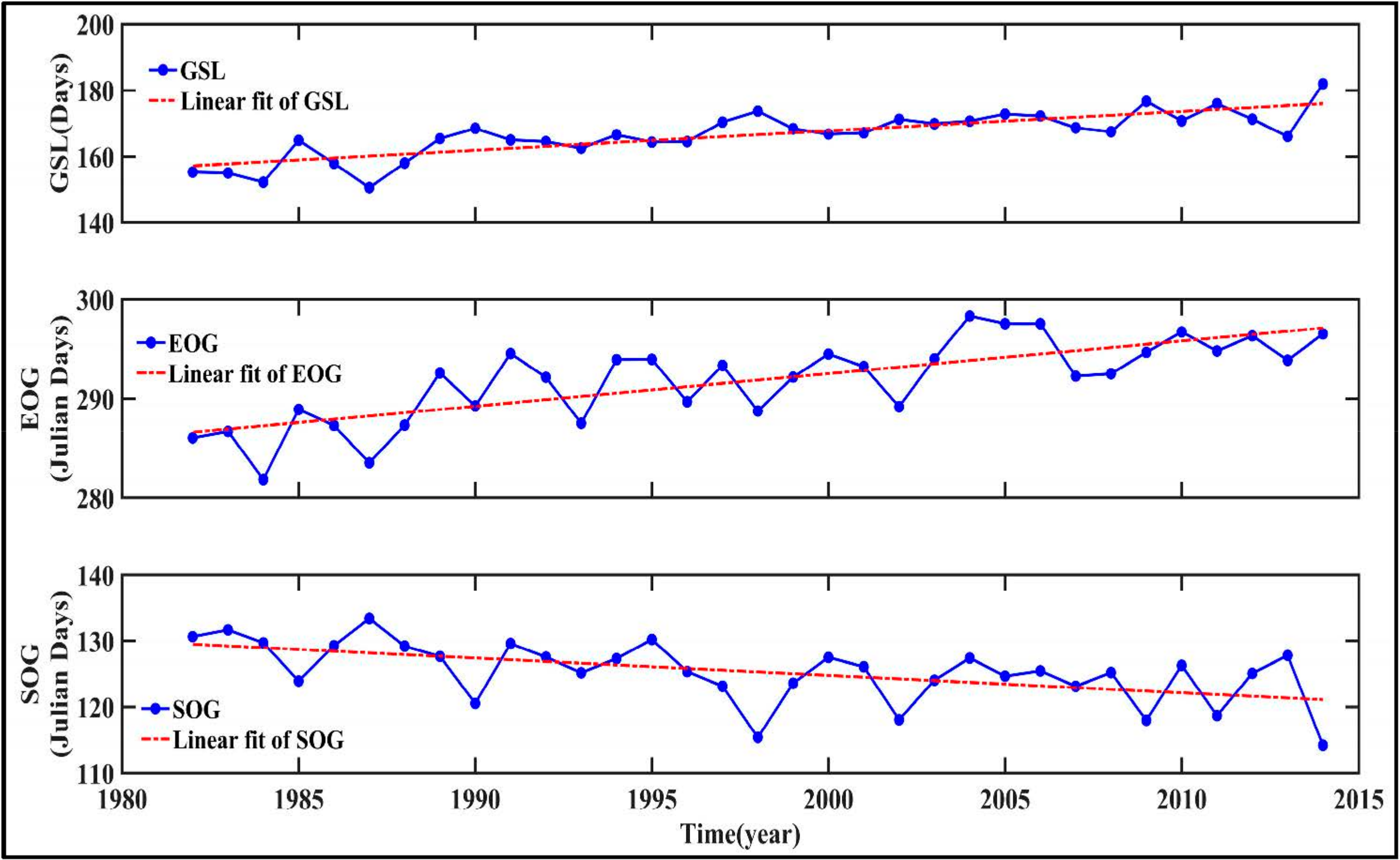
Figure 8.
Correlation coefficient between GSL and AGG in the GKM during 1982–2014. (Green indicates significant positive correlation (r > 0, p < 0.05), brown indicates significant negative correlation (r < 0, p < 0.05), and gray indicates non-significant correlation (p > 0.05)).
Figure 8.
Correlation coefficient between GSL and AGG in the GKM during 1982–2014. (Green indicates significant positive correlation (r > 0, p < 0.05), brown indicates significant negative correlation (r < 0, p < 0.05), and gray indicates non-significant correlation (p > 0.05)).

Figure 9.
Correlation coefficient between Fraction of Photosynthetically Active Radiation (FPAR) and AGG in the GKM during 1982–2014. (Yellow and red indicate significant positive correlation (r > 0, p < 0.05), blue indicates significant negative correlation (r < 0, p < 0.05), and gray indicates non-significant correlation (p > 0.05)).
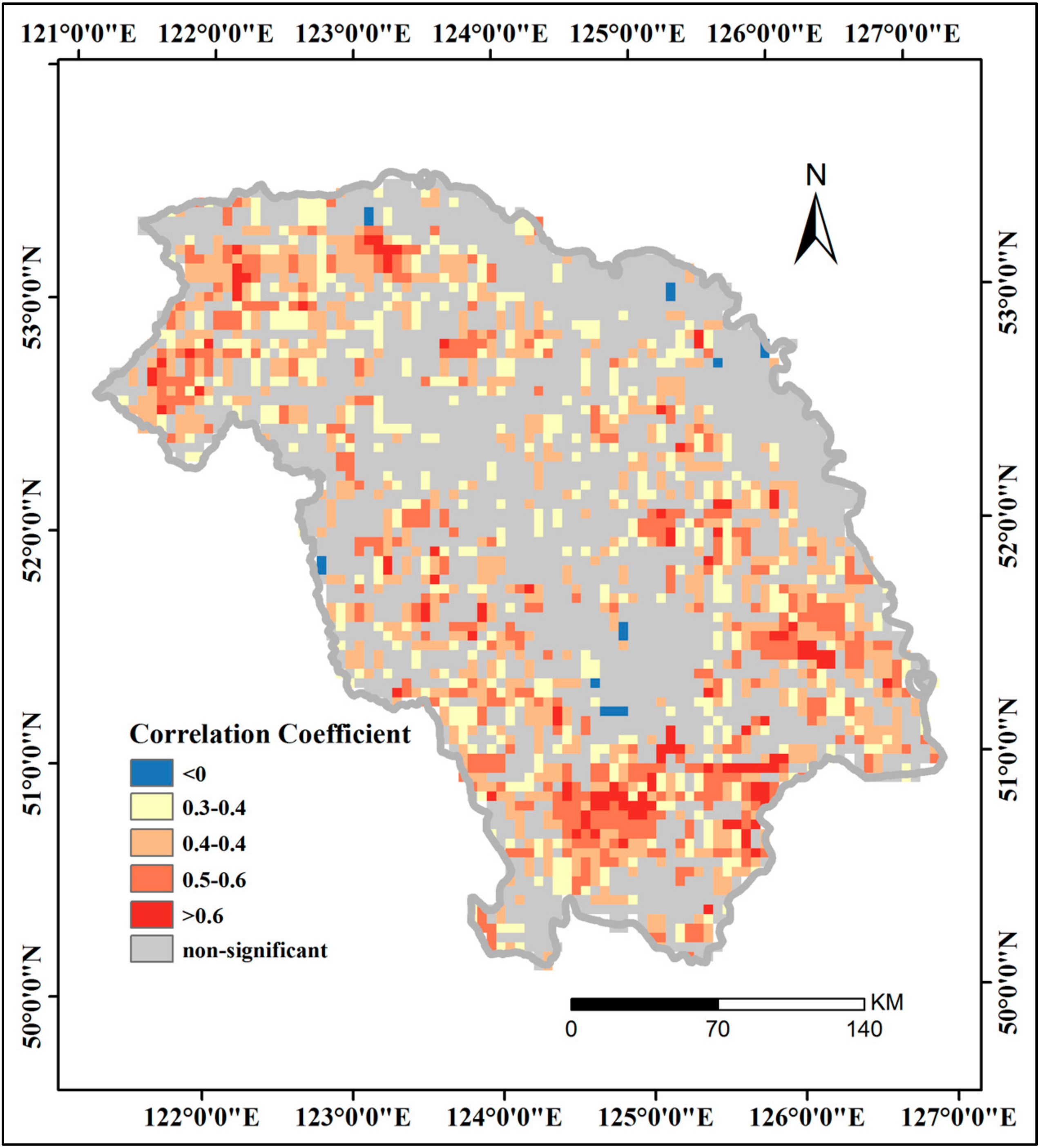
Figure 10.
Spatial distribution of (a) dominant and (b) subdominant factors for AGG in the GKM from 1982 to 2015 (Non-significant means that there is no significantly effective factor for AGG among these five driving factors according to the F-test and t-test. A significant F-test was under p < 0.05, and a significant t-test was under the absolute value of t ≥ 1.96).

Figure 11.
Contrast of AG in specific land cover and other areas in the GKM.
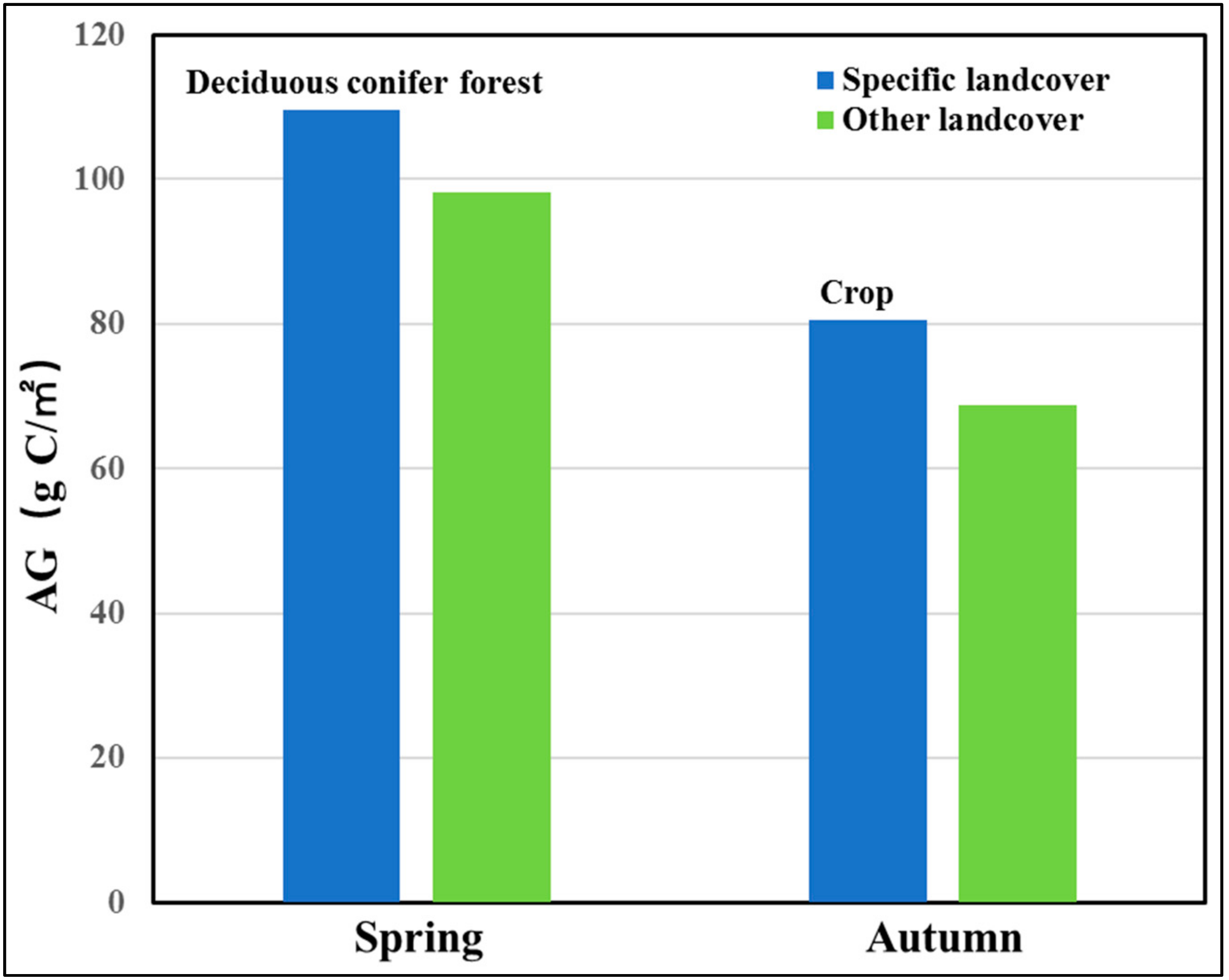
Figure 12.
Variation of AGG with elevation.
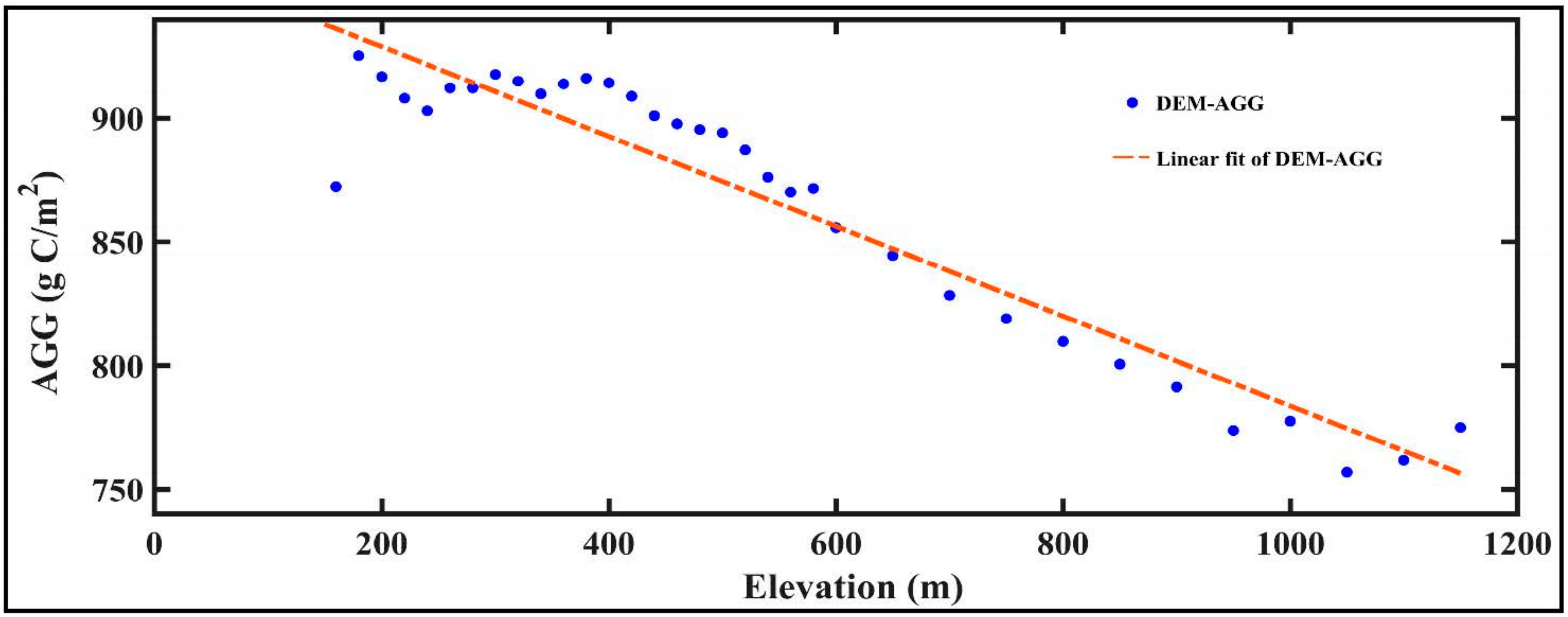
Figure 13.
Variation in annual mean daily temperature and annual mean daily precipitation in the growing season over the GKM from 1982 to 2015.
Figure 13.
Variation in annual mean daily temperature and annual mean daily precipitation in the growing season over the GKM from 1982 to 2015.

Figure 14.
Variation in timber yield in Heilongjiang Province since 1980.

Figure 15.
Burnt zone of the fire in 1987 and land cover in the GKM.

Table 1.
Correlation coefficients of the AG in three seasons and the growing season versus meteorological factors obtained from five different meteorological stations over the GKM from 1982 to 2015.
Table 1.
Correlation coefficients of the AG in three seasons and the growing season versus meteorological factors obtained from five different meteorological stations over the GKM from 1982 to 2015.
| Station | SD | DAT | DMAT | DMIT | DP | |
|---|---|---|---|---|---|---|
| Spring | 50,136 | 0.419 ** | 0.335 * | 0.398 ** | 0.257 | −0.153 |
| 50,246 | 0.279 | 0.435 ** | 0.495 ** | 0.279 | −0.179 | |
| 50,349 | 0.397 * | 0.448 ** | 0.482 ** | 0.292 * | −0.310 * | |
| 50,353 | 0.390 * | 0.381 * | 0.493 ** | 0.200 | −0.150 | |
| 50,425 | 0.295 * | 0.445 ** | 0.419 ** | 0.407 ** | −0.070 | |
| Summer | 50,136 | 0.631 ** | 0.339 * | 0.459 ** | −0.144 | −0.324 * |
| 50,246 | 0.614 ** | 0.669 ** | 0.811 ** | −0.155 | −0.580 ** | |
| 50,349 | 0.814 ** | 0.717 ** | 0.810 ** | −0.017 | −0.482 ** | |
| 50,353 | 0.835 ** | 0.665 ** | 0.753 ** | 0.247 | −0.640 ** | |
| 50,425 | 0.565 ** | 0.590 ** | 0.642 ** | 0.304 * | −0.470 ** | |
| Autumn | 50,136 | 0.474 ** | −0.041 | 0.349 * | −0.255 | −0.608 ** |
| 50,246 | 0.491 ** | −0.026 | 0.410 ** | −0.328 * | −0.484 ** | |
| 50,349 | 0.677 ** | −0.041 | 0.314 * | −0.335 * | −0.441 ** | |
| 50,353 | 0.134 | 0.176 | 0.317 * | −0.051 | −0.429 ** | |
| 50,425 | 0.466 ** | 0.304 * | 0.333 * | 0.206 | −0.447 ** | |
| Growing Season | 50,136 | 0.620 ** | 0.385 * | 0.50,2 ** | −0.055 | −0.371 * |
| 50,246 | 0.587 ** | 0.602 ** | 0.789 ** | −0.137 | −0.544 ** | |
| 50,349 | 0.753 ** | 0.626 ** | 0.773 ** | 0.005 | −0.513 ** | |
| 50,353 | 0.659 ** | 0.604 ** | 0.704 ** | 0.294 * | −0.623 ** | |
| 50,425 | 0.577 ** | 0.572 ** | 0.603 ** | 0.367 * | −0.470 ** |
SD refers to sunshine duration, DAT refers to daily average temperature, DMAT represents daily maximum temperature, DMIT represents daily minimum temperature, and DP represents daily precipitation; * p < 0.05, statistical significance of Pearson correlation; ** p < 0.01, statistical significance of Pearson correlation.
Table 2.
Zonal mean value of the coefficient for each dominant factor.
| Dominant Factor | GSL | FPAR | Temperature | Sunshine Duration |
|---|---|---|---|---|
| Zonal mean coefficients | 0.399134 | 0.453251 | 0.448733 | 0.518619 |
© 2018 by the authors. Licensee MDPI, Basel, Switzerland. This article is an open access article distributed under the terms and conditions of the Creative Commons Attribution (CC BY) license (http://creativecommons.org/licenses/by/4.0/).
Share and Cite
MDPI and ACS Style
Hu, L.; Fan, W.; Ren, H.; Liu, S.; Cui, Y.; Zhao, P. Spatiotemporal Dynamics in Vegetation GPP over the Great Khingan Mountains Using GLASS Products from 1982 to 2015. Remote Sens. 2018, 10, 488. https://doi.org/10.3390/rs10030488
AMA Style
Hu L, Fan W, Ren H, Liu S, Cui Y, Zhao P. Spatiotemporal Dynamics in Vegetation GPP over the Great Khingan Mountains Using GLASS Products from 1982 to 2015. Remote Sensing. 2018; 10(3):488. https://doi.org/10.3390/rs10030488
Chicago/Turabian StyleHu, Ling, Wenjie Fan, Huazhong Ren, Suhong Liu, Yaokui Cui, and Peng Zhao. 2018. "Spatiotemporal Dynamics in Vegetation GPP over the Great Khingan Mountains Using GLASS Products from 1982 to 2015" Remote Sensing 10, no. 3: 488. https://doi.org/10.3390/rs10030488
Note that from the first issue of 2016, this journal uses article numbers instead of page numbers. See further details here.