Article

Leaf and Canopy Level Detection of Fusarium Virguliforme (Sudden Death Syndrome) in Soybean

1
Department of Forest & Wildlife Ecology, University of Wisconsin-Madison, 1630 Linden Drive, Madison, WI 53706, USA
2
Department of Agronomy, University of Wisconsin-Madison, 1575 Linden Drive, Madison, WI 53706, USA
3
Department of Plant, Soil and Microbial Sciences, Michigan State University, East Lansing, MI 48824, USA
*
Author to whom correspondence should be addressed.
Remote Sens. 2018, 10(3), 426; https://doi.org/10.3390/rs10030426
Submission received: 1 February 2018 / Revised: 26 February 2018 / Accepted: 6 March 2018 / Published: 9 March 2018
(This article belongs to the Section Remote Sensing in Agriculture and Vegetation)

Abstract

:
Pre-visual detection of crop disease is critical for food security. Field-based spectroscopic remote sensing offers a method to enable timely detection, but still requires appropriate instrumentation and testing. Soybean plants were spectrally measured throughout a growing season to assess the capacity of leaf and canopy level spectral measurements to detect non-visual foliage symptoms induced by Fusarium virguliforme (Fv, which causes sudden death syndrome). Canopy reflectance measurements were made using the Piccolo Doppio dual field-of-view, two-spectrometer (400 to 1630 nm) system on a tractor. Leaf level measurements were obtained, in different plots, using a handheld spectrometer (400 to 2500 nm). Partial least squares discriminant analysis (PLSDA) was applied to the spectroscopic data to discriminate between Fv-inoculated and control plants. Canopy and leaf spectral data allowed identification of Fv infection, prior to visual symptoms, with classification accuracy of 88% and 91% for calibration, 79% and 87% for cross-validation, and 82% and 92% for validation, respectively. Differences in wavelengths important to prediction by canopy vs. leaf data confirm that there are different bases for accurate predictions among methods. Partial least square regression (PLSR) was used on a late-stage canopy level data to predict soybean seed yield, with calibration, cross-validation and validation R2 values 0.71, 0.59 and 0.62 (p < 0.01), respectively, and validation root mean square error of 0.31 t·ha−1. Spectral data from the tractor mounted system are thus sensitive to the expression of Fv root infection at canopy scale prior to canopy symptoms, suggesting such systems may be effective for precision agricultural research and management.

Graphical Abstract

1. Introduction

Remote and proximal sensing are increasingly applied in agriculture [1] for diverse applications, including estimation of yield [2], water content [3], crop nutrients [4,5,6], leaf area index (LAI; [7,8,9,10]), disease [11,12], pest [13,14,15,16] and soil properties [1]. Here, we test the capacity of tractor-based proximal spectral measurements to detect Fusarium virguliforme (Fv, which causes soybean sudden death syndrome) root infection and assess seed yield of soybeans.
Soybean (Glycine max (L.) Merr.) is the fourth largest commodity crop in the world in terms of area harvested and production. The anticipated increase in demand for soybean over the next 20 years is expected to result in 50% expansion of soybean cultivated land area [17]. Sudden death syndrome (SDS) was among the top yield-suppressing diseases of soybean in the United States from 1996 to 2007 [18], with average annual crop loss in the US assessed to be around $100 million US [19]. In individual fields, yield losses of up to 80% have been attributed to SDS but yield losses of 5 to 15% are more common [20]. Since its discovery in Arkansas in 1972 SDS has spread to much of the soybean growing region of the US, and South America [19,21,22]. The SDS disease cycle starts shortly after planting with infection of roots resulting in reduced root length, surface area, volume, and mass [23]. Fv has not been isolated from aboveground portions of the soybean plant, therefore, assumed not to be present above ground [24,25]. The primary field detection method for SDS is canopy symptoms. Canopy symptoms are the result of fungal phytotoxins translocated from roots to leaves causing Rubisco and chlorophyll degradation, initiation of chlorosis and necrosis in leaves [19,26,27]. Soil temperature and moisture influence early season Fv infection, and canopy symptoms that are most common during the reproductive (late) growth stages [23,28]. The balance between environmental conditions influence on the pathogen and the host plays a role in the severity of the canopy symptoms [29] that can fluctuate from very light chlorosis to necrosis and complete premature defoliation in a matter of days. In cases of no apparent canopy symptoms, the pathogen can remain unnoticed in the soil, infected roots or plant residue as a potential risk for subsequent growing seasons. When canopy symptoms are absent, destructive sampling is used to assess Fv presence on roots [30], pulling the root to look for root rot and cutting lower stems to distinguish from other disease [19,30] or quantitative real-time polymerase chain reaction (qPCR)-based detection [20,31]. There is no in-season treatment for infected plants, making it important to detect Fv infection to take preventive actions in the next planting cycle [32] and consider impact on yield for the current season. Although risk of Fv infection has been studied [33], a nondestructive method to identify Fv infected soybeans prior to visual symptoms is needed.
Field spectroscopy is routinely used to obtain proximal data for crop assessment and phenotyping. Most commonly, one spectrometer obtains target and white reference measurements alternately, with the frequency of white reference measurements dependent on the atmospheric stability. Under variable atmospheric conditions white reference measurements may be difficult to detect at a suitable timing with respect to target measurements to ensure high fidelity and repeatable reflectance spectra. A dual field-of-view system, on the other hand, obtains target and white reference nearly simultaneously, enabling calculation of relative reflectance from down- and up-welling measurements [34,35] that minimize effects of atmospheric variability [36,37]. Referencing by downwelling radiation rather than by white panel can make dual field of view systems mounted on moving measuring platforms more easily applicable. This is important for agricultural applications, as growers may not have the flexibility to await atmospherically clear days, and leaf level measurements using external light sources is time consuming and inefficient.
Proximal measurements using the sun as illumination can be a challenge [36,38]. MacLellan and Malthus [39] presented the concept of a two spectrometers system with dual field of view for each, alternately obtaining upwelling (radiance) and downwelling (irradiance) measurements, using a cosine response fore optic [40] in lieu of the standard white reference. MacArthur et al. [41] designed and presented an operational system (Piccolo) that is lightweight, self-contained, and wirelessly controlled, and similar in principle to dual field of view systems used at eddy covariance towers for canopy reflectance observations [42,43]. Here, for the first time, the two spectrometers Piccolo system [41] is mounted on a moving platform at ground level for a precision agriculture application. As a test of its feasibility we assess the capacity to (1) detect disease status; and (2) predict yield in soybean from proximal visible-near infrared-shortwave infrared spectra (400–1630 nm). Finally, we compare the results from proximal methods to data collected at the leaf level using a handheld spectrometer and external light source.

2. Materials and Methods

2.1. Study Area and Experimental Design

Field experiments were conducted during April to October 2016 at the University of Wisconsin Arlington Agriculture Research Station (43°18′8′′N, 89°20′8′′W) and in Hancock Research Station (44°7′10′′N, 89°32′7′′W). Soils at Arlington are Plano fine-silty, mixed, super active, mesic Typic Argiudoll, and Hancock are Plainfield sand, mixed, mesic Typic Udipsamment [23]. The Hancock site was irrigated to mitigate water stress while the Arlington site was not. No fertilization treatments were applied. The Arlington site included two adjacent experiments, one used for the canopy level (proximal) analyses and the second for the leaf measurements used for comparison, with the leaf study replicated at Hancock. The canopy level experiment was a split-split-plot arrangement with four replications arranged in completely randomized blocks, with three planting dates (Table 1) resulting in non-uniform development stages for most of the measuring dates. Fields were planted with two soybean cultivars (i.e., RS213NR2 and AG2136) and three seed treatments (i.e., untreated control, Poncho®/VOTiVO®, and Poncho®/VOTiVO®/ILeVO®) as detailed by Vosberg et al. [23] at a uniform seed density of 346,000 seeds·ha−1. Each sub-subplot consisted of two inoculation treatments (i.e., inoculated with Fv and untreated control) and encompassed two rows 7.6 m long spaced 76 cm apart. The inoculation treatment in the sub-subplot was the experimental unit and from here on will be designated as “plot”. The total number of plots was 144. The rows were in a north–south orientation and each row had eight plots along it, with 18 plots in the east-west orientation. There were eight alleys (four rows wide each) for the tractor mounted with Piccolo Doppio. To minimize border effects, alleys and borders and any side of the experiment that did not have soy plants next to it and the rest of the field was planted with filler soybean plants cultivar Channel 0906R2 with seed density of 346,000 seeds·ha−1.
Each of the two leaf level experiments (Arlington and Hancock) had four rows 7.6 m long spaced 76 cm apart. Two of the rows were inoculated [23] with Fv and two rows were not inoculated and defined as untreated control. Both sites were planted with AG2136 cultivar and uniform seed density of 346,000 seeds·ha−1. A total of 500 soybean plants were tagged to allow repeated measurements through the growing season, with 125 plants per inoculation treatment per site.

2.2. Data Collection and Processing

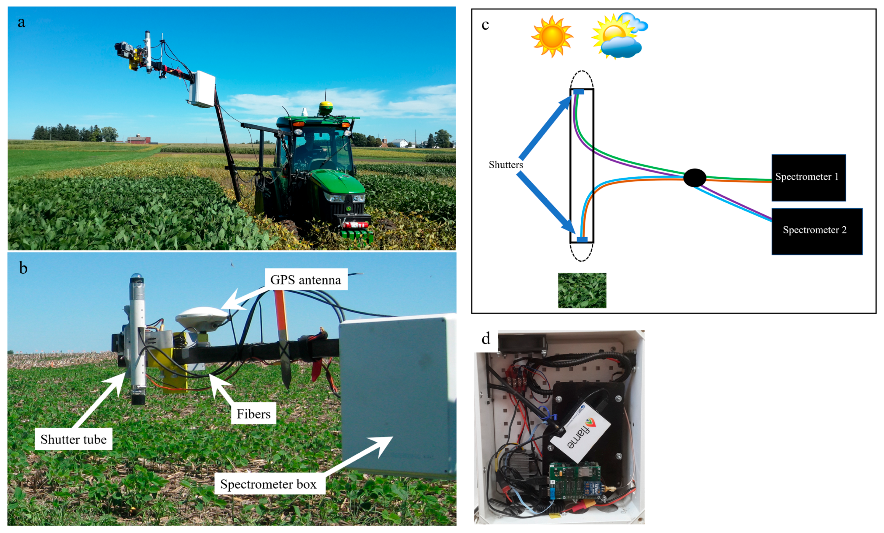
2.2.1. Canopy Spectral Data Collection and Processing

The canopy spectral data were obtained through the growing season (Table 1) by a tractor mounted Piccolo Doppio dual field-of-view two-spectrometer system [41] equipped with two spectrometers: Flame and NIRQuest (Ocean Optics, Inc., Dunedin, FL, USA). The Flame had a spectral range of 340 to 1022 nm with an optical resolution of 1.33 nm full-width half-maximum (FWHM) interpolated to 1 nm spacing. The range of 400 to 900 nm was used due to noisy data at the longest and shortest wavelengths. The NIRQuest has a spectral range of 900 to 1713 nm with an optical resolution of 6.6 nm FWHM interpolated to 1 nm resolution, with 900 to 1630 nm used due to noisy data at the longest wavelengths. The ability to obtain upwelling and downwelling data almost simultaneously derives from the use of two fiber optics with diameters of 400 μm and 600 μm, respectively, which together completely cover the 1 mm long and 25 μm wide inlet slit of the Flame spectrometer (Figure 1). An identical set of fiber optics was used for the NIRQuest that had a 1 mm long and 100 μm wide inlet slit, also fully covered by the two fiber optics.
The upward and downward facing fibers were attached to a custom two-axis gimbal fitted onto the boom to maintain nadir orientation. As detailed by [41], the downwelling (upward looking) fiber viewed the sky through a cosine corrected polytetrafluoroethylene fore-optic and glass dome, while the upwelling (downward looking) bare fiber (view angle was 25 degrees) was fit with only an optical glass dome (Figure 1). Each optic was fitted with a shutter to obtain data via one of the fibers at a time. Synchronizing shutter activity and integration times of the spectrometer was controlled by a Raspberry Pi (Raspberry Pi Foundation, Cambridge, UK) single-board computer [41]. The Raspberry Pi time-stamped each spectral measurement. For spectra geo-referencing location and time every second, a GPS receiver (Geo 7x, Trimble, Sunnyvale, CA, USA) in the tractor’s cabin connected to a GNSS antenna mounted on the boom, behind the shutter tube (Figure 1). The GPS data were differentially corrected in Pathfinder software (Trimble Inc., Sunnyvale, CA, USA) using the reference base UNAVCO, Iowa County, WI located at 42°54′51′′N, 90°14′53′′W, 294 m above sea level. The estimated accuracy ranged from 5 to 15 cm for 99.96% of the corrected positions. Spectral data were collected within two hours of solar noon from a single row per pass with a total of two passes (i.e., two rows) per plot and collection date. The upwelling fiber was centered on the soybean row 25 cm above the top of the canopy resulting in ~12 cm diameter at top of canopy. The system was on for at least 40 min prior to starting measurements. The Flame integration times were 5 and 15 ms and the NIRQuest integration times were 700 and 1000 ms for downwelling and upwelling, respectively. The integration times were set based on visual examination of the obtained spectral reflectance to maximize the signal while avoiding saturation under variable sky conditions (defined as 75% of maximum DN count). To minimize the time gap between upwelling and downwelling data collection and between spectrometers, the eight-measurement sequence was: (1) Flame upwelling dark current; (2) NIRQuest upwelling dark current; (3) upwelling radiance by Flame; (4) upwelling radiance by NIRQuest; (5) downwelling irradiance by Flame; (6) downwelling irradiance by NIRQuest; (7) downwelling dark current by Flame; and (8) downwelling dark current by NIRQuest. Tractor speed was set to 0.22 m s−1 and actual time between the starting point of each set of eight measurements was approximately ~6.7 s resulting in potential of five spectra collected per plot row.
ArcGIS 10.3 (Environmental System Research Institute, Redlands, CA, USA) was used to spatially relate each 1 s GPS time stamp to a plot relying on plots polygon shape file. Time stamps with distances less than 0.22 m from the border of the plot were excluded to assure that both Flame and NIRQuest obtained targets within the experimental plot setup. Relative reflectance values for each plot were obtained using a custom Python script (https://github.com/prabu-github/tracolo). Dark current was subtracted from the upwelling radiance and downwelling irradiance spectra, and then the radiance was divided by the irradiance, while accounting for fiber diameter, integration time and field of view:
R = ( D N u p D N u p d a r k ) [ I T u p ( π r u p 2 ) ( π F O V u p 180 ) ] ( D N d o D N d o d a r k ) [ I T d o ( π r d o 2 ) ( π F O V d o 180 ) 2 π ]
where R is relative reflectance; DN is the spectral data of one sample (vector) and the units are digital number; dark stands for dark current spectral data; up and do stands for upwelling and downwelling, respectively; IT stands for integration time in ms; r stands for the radius of the fiber optic in μm; and FOV stands for field of view of the fiber optic in degrees. The process presented in Equation (1) was applied for spectral data from each of the spectrometers separately. The 1 nm relative reflectance data were averaged per plot, smoothed by using the Savitzky and Golay [44] filter with a 5 nm window and polynomial degree of 2 for the 1 nm resolution, then, the reflectance were resampled to 5 nm resolution for each of the spectrometers separately. Resampling resulted for the Flame in reflectance values for 101 bands ranging from 400 to 900 nm and for the NIRQuest in reflectance values for 147 bands ranging from 900 to 1630 nm. Spectral data, from each of the spectrometers, were then vector normalized by instrument to minimize the disparity in intensity levels [45]. The vector normalized spectra from the same plot and measuring date of both spectrometers were merged at 900 nm. Merging was performed by subtracting the NIRQuest reflectance value in 900 nm from the averaged reflectance of 880–900 nm and adding this scalar to the normalized reflectance values of all NIRQuest wavelengths, resulting in merged spectra with 247 bands in 5 nm resolution in the range of 400 to 1630 nm.

2.2.2. Leaf Spectral Data Collection and Processing

The leaf spectral data were acquired in vivo throughout the growing season (Table 1) using an ASD FieldSpec3 full-range (350 to 2500 nm) spectrometer with leaf clip (Analytical Spectral Devices, Boulder, CO, USA) and a tungsten halogen light source. The spectrometer and light source were on for at least 40 min prior to measuring and white reference measurements were obtained every 10 min using a spectralon panel. The adaxial side of the terminal leaflet of each trifoliate leaf was measured three times: right side, left side and far from the petiole at the center (where the leaf vein is relatively thin), with each measurement consisting of an average of 10 spectra. For the vegetative stages, the newest fully developed leaf was measured, until 5 July 2016. During the reproductive stages that followed, the same terminal leaflet was tagged and remeasured (Table 1) each date, until 8 August 2016. The newest fully developed leaf was measured again in the last measuring date for each of the sites because of damage to the relatively old leaves. In case the middle leaflet was missing or damaged, one of the other two leaflets was measured. To avoid time of day biasing in sampling, measurements were alternated between rows of different treatments. Near the end of the growing season, outburst natural outbreak of SDS occurred in hundreds of plants ~100 m north of the Arlington experiment, in the filler of the same field, and were also measured to get example spectra of symptomatic plants (Table 1), including both chlorotic and green areas on the leaflet. These leaves measured at the top of the canopy. Leaf spectral data were processed using the SpecDAL python package (https://github.com/EnSpec/SpecDAL), with the final data set using 400 to 2500 nm at 5 nm spacing.

2.2.3. Root Samples for Quantitative Real-Time Polymerase Chain Reaction (qPCR)

Root samples were collected from the leaf level experimental plots to determine the absolute abundance of Fv (Table 1). Root samples were separated from the plant, washed, and dried at 65 °C for at least 48 h. Samples were homogenized to pass through a 0.5 mm sieve and stored at 4 °C until DNA extraction. DNA was extracted, quantified and qPCR was conducted to obtain absolute quantity of Fv DNA in root samples, resulting in Fv DNA (pg) per root DNA (ng) as conducted by Wang et al. [31]. A total of 79 root samples analyzed included: 16 Fv-inoculated samples from Arlington with, 20 control samples from Arlington, 6 samples from Arlington fill, 21 Fv-inoculated samples from Hancock, and 16 control samples from Hancock.

2.3. Data Analyses

2.3.1. Normalized Difference Spectral Indices

Normalized difference spectral index (NDSI) is the normalized difference of all possible two-band combinations in a defined spectral range (Equation (2); [46]). The NDSIs were calculated to assess the relation between two bands combinations of canopy spectral data to discriminate inoculation status and to assess Fv root abundance by leaf spectral data. NDSI values can range from −1 to 1 while the normalization is effective in standardizing the spectral response to observed targets [46].
NDSI = R i R j R i + R j
where R is reflectance in the subscripted wavelength i or j that represents all possible wavelengths between 400–1630 nm for the Piccolo (247 bands at 5 nm resolution; 30,381 combinations) and 400–2500 nm for the ASD (421 bands; 88,410 combinations). Regression was used to identify the NDSI’s best correlated with Fv root abundance, with the coefficient of determination (R2) and root mean square error (RMSE) used as quality metrics. The t-Test was used to identify NDSI’s that discriminated inoculation status (i.e., 0 for untreated control and 1 for inoculated). The analyses were conducted in R 3.4.1.

2.3.2. Partial Least Squares

Partial least squares regression (PLSR; [47,48,49]) was applied to assess the ability of canopy spectral data to predict soybean seed yield, and to assess Fv abundance based on qPCR of soybean root powder. PLS discriminant analysis (PLSDA; [50]) was implemented to classify Fv inoculation status of soybean plants on each of the canopy and leaf level by measurement date and site.
The canopy data had four replicates, one of them was set aside for independent validation. The samples from the other three replicates were internally cross-validated on 100 permutations of the data, using a random 70%/30% split, resulting with 100 calibration and cross-validation models. These 100 calibration models were implemented on the set aside independent validation data resulting in 100 independent validations. The calibration, cross-validation and independent validation results were each presenting averaged quality evaluation means. For the PLSR models the quality evaluation was by R2 and RMSE were obtained to evaluate the models. For the PLSDA models the quality evaluation was by full confusion matrices, total accuracies and Cohen’s Kappa. For both model types, PLSR and PLSDA, the accuracy of quality evaluators was assessed by standard deviation, over the 100 permutations. The leaf data had 25% of the samples randomly set aside for independent validation. The rest of the samples were internally cross-validated on 100 permutations of the data, using a random 70%/30% split, resulting with 100 calibration and cross-validation models. These 100 calibration models were implemented on the set aside independent validation data resulting in 100 independent validations. The calibration, cross-validation and independent validation results were each presenting averaged quality evaluation means and their standard deviation as done for the canopy data. The only exception is the PLSR, leaf data, analysis for Fv root content that did not have independent validation. The standardized coefficients and variable importance in projection (VIP; [48]) statistic of the PLSDA and PLSR models were to determine the relative importance of different wavelength regions to prediction, and as a basis to interpret chemical and physical traits driving the empirical models. Canopy symptoms were identified for the first time on 10 August and a total of 25 of the 144 plots had visual symptoms during the rest of the season. Therefore, canopy level PLSDA models for 15, 22 August, and 2 September were calibrated, cross-validated and validated exclusively using non-canopy symptomatic plots. For the PLSDA models in cases where models performed similarly for the same (or nearly the same) growth stage, data were merged (leaf and canopy were not mixed) and analyzed to test whether general predictive models could be obtained. For all classification analyses using PLSDA we also implemented randomized models in which the classification variable was assigned randomly to the actual spectra. Classification were run on these with 100 permutations and in no cases, did the accuracies of these randomized datasets generate spurious accurate classifications (data not shown). All PLSR and PLSDA analyses were conducted in R 3.4.1. [51].

3. Results and Discussion

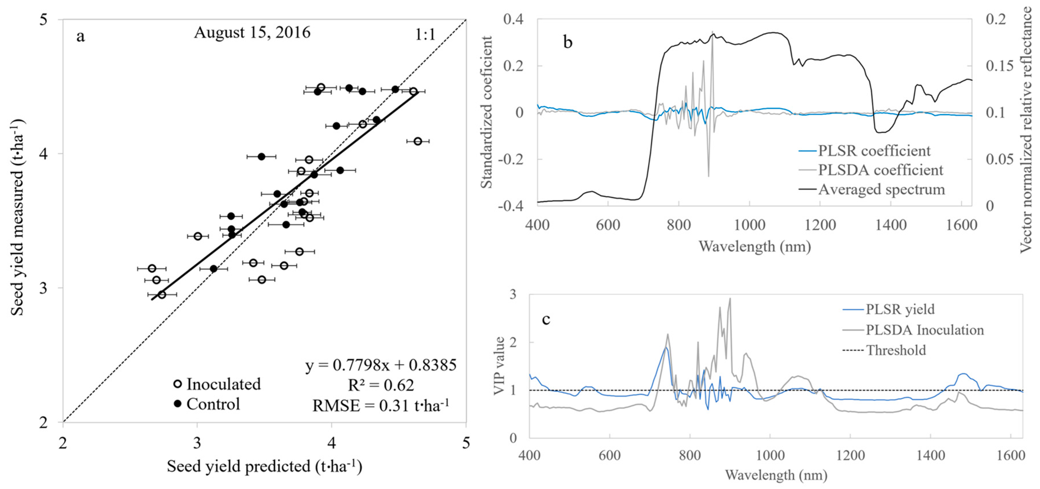
3.1. Spectral Identification of Inoculation—Canopy Level

Data from all canopy level measuring dates (Table 1) were analyzed per date as well as pooled in several combinations. The relevant dates and combinations are presented in Table 2. The confusion matrices indicate reasonable and consistent performance across all treatments, suggesting stable spectral models. The full confusion matrix for all canopy measuring dates in Table 1 and models in Table 2 are in Supplementary Materials S1. The validation total accuracies seasonal trend is discussed in Section 3.3. The best PLSDA classification of inoculation status overall was for plants during all vegetative stages resulting in 77% validation total accuracy (Table 2). The top PLSDA classification of inoculation status for specific dates was based on canopy spectra utilized data from 18 July and 26 July both prior to appearance of canopy symptoms, producing 82% validation accuracy (Table 2). Of note, the two models (18 and 26 July) show very similar patterns (Figure 2), with the red-edge, in 745 and 750 nm in particular having similar VIP scores (Figure 3). The model presenting the data from 18 and 26 July together (Table 2) shows similar validation total accuracy of 75% and similar standardized coefficients as well as VIP scores (not presented). By the quality of classification, the best stages to obtain spectral data for inoculation analysis are late vegetative and early reproductive.
Averaged canopy spectra for inoculated and control plants (Figure 2) show higher reflectance for inoculated plants starting around 860 nm and to the longer wavelengths, especially in the 1400 nm water absorption band. This is related to lower water content in the inoculated plants. From 750–860 nm, the inoculation treatment generally has lower reflectance values which we attribute to a smaller, less green, canopy caused by Fv [52]. The standardized PLSDA coefficients (Figure 2) corroborate the importance of red-edge and near infrared (NIR) wavelengths (750–900 nm) to the prediction of inoculation status, also evident in the VIP statistic (Figure 3). In support with the NIR importance, NDSI t-Test of all 2-band combinations between inoculated and control treatments was applied for spectral data from all dates together (Table 1). The highest t values, significant at p < 0.05, were for band combinations using the NIR at wavelengths between 755 to 1100 nm (summarized in supplemental Figure S2). The NIR importance was expected, at the canopy level, the NIR is influenced primarily by cumulative plant biomass [53] and Fv root infection was negatively affecting root and aboveground biomass development [52,54]. The variability in the standardized coefficients indicates the importance of narrow spectral sampling. At the canopy level, the red-edge provides indication of plant condition that might be related to a variety of traits such as chlorophyll content, water content, leaf area index, seasonal patterns and canopy biomass [55,56,57,58]. The averaged spectrum of non-symptomatic plants in inoculated plots show higher relative reflectance values in the chlorophyll absorption band [59] which is explained to a lesser extent by chlorophyll content as a result of chlorophyll reduction by root infection and possibly phytotoxins in the canopy [27,60]. The vegetative model might be the correct stage, with multiple measuring dates, to assess Fv infection if the pathogen is already established and affecting the root and canopy systems and other canopy influences (e.g., disease, insect damage and senescence) have lesser chance to reduce accuracy of the model than in later stages.

3.2. Leaf Level Spectral Analyses

3.2.1. Spectral Identification of Inoculation—Leaf Level

Data from all leaf level measuring dates and both sites (Table 1) were analyzed to classify inoculated and control treatments per date and site, as well as pooled across several combinations. The confusion matrices indicate reasonable and consistent performance across treatments, suggesting stable spectral models. The full confusion matrix for all leaf measuring dates in Table 1 and models in Table 3 are in Supplementary Materials S3. PLSDA models based on leaf level data were able to discriminate inoculated plants with high level of accuracy on individual dates across sites starting at late vegetative stages to the end of the season in Arlington and to mid-development stages in Hancock. The validation total accuracies seasonal trend is discussed in Section 3.3.
The PLSDA VIP values (Figure 4e) for the Arlington and Hancock models have similar trends, although the standardized coefficients do not (Figure 4a,c). Therefore, data of the same development stages from the two sites were pooled together and analyzed, resulting in total accuracies of ~50% to classify the two Fv inoculation status (data not presented), likely because of fundamental differences between the two field sites that affected overall phenotype of the plants. For example, water and soil dynamics are dramatically different between Hancock (sandy soils, therefore, irrigated) and Arlington (fine silty and not irrigated). To test this, we used PLSDA to discriminate between plants at Arlington and Hancock, resulting in total accuracies that are all higher than 91% for calibration, cross-validation and validation models. The important VIP bands are mainly in the visible, red-edge and SWIR water absorptions, showing the influence of environmental conditions including Fv abundance in soybean roots (full confusion matrices and VIP values in Supplementary Materials S4). As such, under different environmental conditions, phenotypic variation within the same genotype can obscure the ability to implement a general algorithm for disease detection [61,62]. Some of the phenotypic variation in spectral response and resulting equations likely also related to the Hancock plants are irrigated while Arlington plants are rain fed. Although there is no visual change in reflectance values in 670 nm, chlorophyll reduction by phytotoxins translocated to the canopy [27] or by root infection affecting the plant health [52] may explain the difference between the reflectance values of the inoculation status around 550 nm and of the slope between 550 to 670 nm. Gitelson and Merzlyak [59] reported higher reflectance in the 550 to 670 nm slope for minor chlorophyll reduction and changes in 670 nm reflectance only after relatively high changes in chlorophyll. These distinctions in the visible wavelengths were apparent despite no visual SDS canopy symptoms present at the time of sampling, and no visual differences between the treatments in the field. Examining the presented models in Figure 4e, the visible blue and red and red-edge spectral regions were most important in all the cases. The water bands at 1400, 1900 and 2500 nm also show minor relevance. The leaf level analyses in general result in different models by date and study site, using VIP and standardized coefficients as diagnostics. The models show general similarities in the regions that are important, and the analyses indicate sensitivity of leaf spectra to Fv inoculation status. In order to obtain the highest quality of classification there is a need to analyze specific and sequential development stages for specific site induced environmental conditions. One of the differences between sites is also Fv natural abundance.

3.2.2. Spectral Assessment of Fv Abundance in Root by Leaf Measurement

We further analyzed the qPCR results to assess whether disease abundance in the root system expressed a range of response in foliar spectra, using PLSR. Spectra appear to show some sensitivity to degree of infection, with a cross-validation R2 of 0.47 and RMSE of 3.2 pg/ng (calibration R2 of 0.53 and RMSE of 2.8 pg/ng; Figure 5a). The highest standardized PLSR coefficients of the model (Figure 5b) were in the visible wavelengths, peaking around the chlorophyll absorption band at 670 nm [59]. The standardized coefficients in the visible range were mainly positive, indicating that reflectance in the red wavelengths correlated positively with Fv abundance, meaning higher reflectance values are related to lower chlorophyll content and higher Fv in roots. The NDSI analysis (Figure 5e) identified the index with the highest relation to Fv root abundance at 690 and 1390 nm, wavelengths strongly influenced by chlorophyll and water absorption [63], respectively. The differences in Fv abundance between Arlington and Hancock (Figure 5d) are suggested to be partly related to a larger difference between the inoculated and control averaged spectra for Arlington than for Hancock (Figure 4b,d) as seen in the 550 to 670 nm slope. The area of the natural outbreak of Fv 100 m from our experimental plots had much higher qPCR detected disease in the roots (Figure 5c), so it is likely that larger ranges of infection than shown in our experiment would yield even greater spectral responses due to effects on foliage. Of note, the presence of a natural infection near our experiment makes it possible that Fv infection was present at a low level in the control plants (see Figure 5c), which makes our results more remarkable that were able to discriminate and validate treatments.
To the best of our knowledge this is the first study showing quantitative assessment of Fv abundance in soybean roots by leaf full range (400 to 2500 nm) hyperspectral data. This is one of the few studies to detect Fv infection via foliage measurements prior to visual sudden death syndrome foliar symptoms [60,64]. Roth et al. [60] demonstrated reduced chlorophyll content in soybean leaves prior to visual sudden death syndrome symptoms, using the newly developed MultispeQ sensor [64], which provides credence to our findings. Using hyperspectral sensor and MultispeQ data together, there is the potential to improve the ability to detect Fv abundance prior to visual symptoms.

3.3. Piccolo Performance

The ability to spectrally discriminate between Fv inoculated and control soybean plants varies during the growing season (Figure 6). However, the time of season with the best discrimination quality is consistent. The season starts with low discrimination accuracy likely because Fv had not yet established itself on the root system sufficiently to affect detectable aboveground properties [52]. As Fv establishes itself in the root system, its effect becomes detectable, perhaps at the leaf level a bit sooner than the canopy. Later in the season in late reproductive stages the total accuracies of Arlington canopy and Hancock leaf plots drop, as the Fv effect on the canopy is masked by processes affecting both control and inoculated plants, such as general senescence, other diseases, pests or physical damage to the foliage. Interestingly, the Arlington canopy models excluding plots with canopy symptoms had higher accuracies than the models including symptomatic plots. This supports the ability to discriminate prior to visual canopy symptoms using NIR bands (Figure 2 and Figure 3), and due to the differences in the models that this capacity for detection is a consequence of the non-visual cues. Processes affecting both control and inoculated plants can affect the leaf level as well. For example, the Hancock leaf plot suffered from white mold (Sclerotinia sclerotiorum) infection starting late in the season, while the Arlington leaf plot maintained relatively high total accuracies through the last measuring date. As well, the qPCR analyses showed Fv abundance significantly higher for the Arlington compared to Hancock plot (Figure 5d), suggesting that it was much less likely that the Fv effect was not masked and, thus, was spectrally detected at Arlington in late reproductive stage. Both measurement strategies, leaf and canopy, have resulted in high quality of discrimination between inoculated and control plots. Discrimination by each strategy was based on different biophysical properties and captured by different spectral features. The canopy level captures differences in above ground canopy biomass. The leaf level is capturing the non-visual differences in pigmentation that are not detected by canopy level data. Both strategies capture some relative importance of bands related to water content. Leaf level measurements can readily be used for specific locations or to predict level of root Fv infection, while the Piccolo is spectrally suitable for Fv infection detection in field and being tractor mounted made it a potential tool also for other precision agriculture applications.
The major effect of disease on crops is reduced yield, so we tested whether the spectral data also could predict the concomitant effects of Fv on yield. Seed yield ranged from 2.02 to 5.21 t·ha−1, with the average seed yield of the inoculated (3.68 t·ha−1) 6% smaller than control (3.91 t·ha−1) treatment (statistically significant at p < 0.05; [23]). Canopy spectral data from each of the measurement dates were used to calibrate, cross-validate and validate PLSR models of seed yield (Supplementary Materials S5), with the best model based on the 15 August data having a reasonable R2 values of 0.71, 0.59 and 0.62 and RMSE of 0.35, 0.41 and 0.31 t·ha−1 for calibration, cross-validation and validation, respectively (Figure 7a). The important spectral wavelengths for prediction were at the red-edge (Figure 7b,c), supporting observations by Christenson [65]. The red-edge was also important for predicting inoculation status, but the NIR bands were more prominent for disease detection, whereas yield prediction was driven largely by red-edge reflectance (Figure 7b,c). There is a long history of field spectroscopy use for yield detection. In soy, Ma et al. [66] used a handheld multispectral spectrometer to correlate vegetation indices to soybean seed yield, with R2 from 0.44 to 0.80 on a range of yield 1 t·ha−1 to > 4 t·ha−1 (but no cross-validation or validation were applied, nor RMSE reported). Yu et al. [67], resulted in correlation coefficient (r) of 0.82 for airborne multispectral imagery data and soybean seed yield correlation. Christenson [65] obtained canopy spectral data and resulted in R2 of 0.58 with RMSE of 0.7 t·ha−1 for a yield ranging from less than 1 t·ha−1 to > 5 t·ha−1. The smallest RMSE of validation obtained for the best PLSR model (Supplementary Materials S5) in the current study is 0.31 t·ha−1 less than half of presented by Christenson [65]. These and other studies show that spectral data are effective for reliable and rapid yield assessments, with reasonable results here in the context of disease infestation. The tractor mounted Piccolo system provides the spectral range needed to feasibly detect Fv root infection and predict seed yield.
There is some remaining noise in canopy spectral data (Figure 2 and Figure 4b) the effect it has on the PLS models is visual in the VIP data (Figure 3 and Figure 4c). This effect is assumed not to interfere with the importance of the spectral regions of the discrimination and prediction models but to have more of an effect on the importance of specific narrow bands as for the NDSI selection. Therefore, for future reflectance data preprocessing, the Whittaker smoother [68,69] will be explored for its build in filter optimization. It is expected that the Whittaker smoothing algorithm will improve analyses accuracy.
The Piccolo system provided an efficient method for the collection of plant reflectance by eliminating the need for frequent reference standard measurements. The ability to obtain relative reflectance under changing atmospheric conditions makes the Piccolo system a reasonable approach for field sampling, especially in a research setting. The system utilized in this study collected reflectance from a single row during each pass; additional efforts to streamline the system for more rapid data acquisition would be required to make this practical in a commercial application. For example, future modifications and deploying more than one system would enable the measurement of plant reflectance from a larger area such as the entire width of a ground sprayer. Alternately, deployment from an unmanned aerial vehicle would also expand the utility of the system. Simultaneous acquisition from both spectrometers would also reduce the minimum time between data acquisition.

4. Conclusions

Crop phenotyping is a bottleneck in plant research, and rapid methods to assess disease, yield and other traits for large numbers of samples are needed. Seed yield is one of the most critical traits that can be spectrally assessed [2,70], although—unlike disease which is detectable due to physiological effects on foliage—detection of yield is based on indirect correlations with physiology. Our study showed promising results for use of spectral sensing of the canopy and leaves to identify Fv infection on soybean roots where no canopy symptoms are visually present. To the best of our knowledge this is the first publication that documents ability to discriminate Fv-inoculated soybean plants from control plants by visible, NIR and SWIR hyperspectral data in canopy and leaf level prior to canopy symptoms. We conclude:
  • Fv inoculation that accrues in the roots can be spectrally detected in the soybean foliage at the canopy and leaf scales as demonstrated by distinguishing between inoculated and control plots and plants, respectively.
  • Early reproductive stage is the recommended timing for canopy level measurements to distinguish between inoculated and control plots.
  • Late vegetative and early reproductive stages are the recommended timings to distinguish between inoculated and control plants at the leaf level.
  • Fv abundance in soybean roots can be spectrally assessed by leaf hyperspectral data.
  • The dual field-of-view system produced canopy spectral data resulting in our ability to spectrally distinguish between Fv inoculation treatments and assess seed yield, thus, showing feasibility of operation for precision agriculture research and potential commercial applications.
For future work, qPCR samples should be collected over the course of the growing season to provide a better understanding of the spectral discrimination over time.

Supplementary Materials

Spectral data and associated metadata for this project can be downloaded from EcoSIS.org (https://ecosis.org/#result/2a9d952a-5a28-47b3-9f85-8aa6e6808991; DOI in progress).

Acknowledgments

All sources of funding of the study should be disclosed. Please clearly indicate grants that you have received in support of your research work. Clearly state if you received funds for covering the costs to publish in open access Research support for SC, IH and SV were provided by the Wisconsin Soybean Marketing Board. Support for PT, AS and PR was provided by the NASA Advanced Information Systems Technology program (grant NNX15AN25G) and Terrestrial Ecology program (NNX13AK85A), with additional support to all researchers from the Wisconsin Soybean Marketing Board and USDA Hatch (WIS01874). Partial support for HXC and MC was provided by the Michigan Soybean Promotion Committee. The authors would like to thank Clayton Kingdon for efforts in the field, lab and with the Piccolo to make this work possible; to Alasdair MacArthur and Iain Robinson for their support of the Piccolo instrumentation; to John Gaska for designing and fabricating the tractor mounted boom; to Adam Roth for his help and advice; and Damon Smith for sudden death syndrome insights helping to structure the leaf experiment.

Author Contributions

I.H., S.K.V., S.P.C. and P.A.T. conceived and designed the experiments; I.H. and S.K.V. performed the experiments and collected spectral data and destructive samples; S.K.V. and S.P.C. obtained agronomic data; H.-X.C. and M.I.C. obtained qPCR data; I.H. analyzed spectral data; I.H., P.R., A.S. and P.A.T. contributed preprocessing and analysis tools for spectral data; I.H., H.-X.C., M.I.C., S.P.C. and P.A.T. wrote the paper.

Conflicts of Interest

The authors declare no conflict of interest. The founding sponsors had no role in the design of the study; in the collection, analyses, or interpretation of data; in the writing of the manuscript, and in the decision to publish the results.

References

  1. Mulla, D.J. Twenty five years of remote sensing in precision agriculture: Key advances and remaining knowledge gaps. Biosyst. Eng. 2013, 114, 358–371. [Google Scholar] [CrossRef]
  2. Weber, V.S.; Araus, J.L.; Cairns, J.E.; Sanchez, C.; Melchinger, A.E.; Orsini, E. Prediction of grain yield using reflectance spectra of canopy and leaves in maize plants grown under different water regimes. Field Crop. Res. 2012, 128, 82–90. [Google Scholar] [CrossRef]
  3. Bonfil, D.J.; Karnieli, A.; Raz, M.; Mufradi, I.; Asido, S.; Egozi, H.; Hoffman, A.; Schmilovitch, Z. Rapid assessing of water and nitrogen status in wheat flag leaves. J. Food Agric. Environ. 2005, 3, 148–153. [Google Scholar]
  4. Christensen, L.K.; Bennedsen, B.S.; Jorgensen, R.N.; Nielsen, H. Modelling nitrogen and phosphorus content at early growth stages in spring barley using hyperspectral line scanning. Biosyst. Eng. 2004, 88, 19–24. [Google Scholar] [CrossRef]
  5. Herrmann, I.; Karnieli, A.; Bonfil, D.J.; Cohen, Y.; Alchanatis, V. SWIR-based spectral indices for assessing nitrogen content in potato fields. Int. J. Remote Sens. 2010, 31, 5127–5143. [Google Scholar] [CrossRef]
  6. Pimstein, A.; Karnieli, A.; Bansal, S.K.; Bonfil, D.J. Exploring remotely sensed technologies for monitoring wheat potassium and phosphorus using field spectroscopy. Field Crop. Res. 2011, 121, 125–135. [Google Scholar] [CrossRef]
  7. Asrar, G.; Fuchs, M.; Kanemasu, E.T.; Hatfield, J.L. Estimating absorbed photosynthetic radiation and leaf-area index from spectral reflectance in wheat. Agron. J. 1984, 76, 300–306. [Google Scholar] [CrossRef]
  8. Gitelson, A.A. Wide dynamic range vegetation index for remote quantification of biophysical characteristics of vegetation. J. Plant Physiol. 2004, 161, 165–173. [Google Scholar] [CrossRef] [PubMed]
  9. Nguy-Robertson, A.L.; Peng, Y.; Gitelson, A.A.; Arkebauer, T.J.; Pimstein, A.; Herrmann, I.; Karnieli, A.; Rundquist, D.C.; Bonfil, D.J. Estimating green LAI in four crops: Potential of determining optimal spectral bands for a universal algorithm. Agric. For. Meteorol. 2014, 192, 140–148. [Google Scholar] [CrossRef]
  10. Herrmann, I.; Pimstein, A.; Karnieli, A.; Cohen, Y.; Alchanatis, V.; Bonfil, D.J. LAI assessment of wheat and potato crops by VENμS and Sentinel-2 bands. Remote Sens. Environ. 2011, 115, 2141–2151. [Google Scholar] [CrossRef]
  11. Mahlein, A.K.; Rumpf, T.; Welke, P.; Dehne, H.W.; Plumer, L.; Steiner, U.; Oerke, E.C. Development of spectral indices for detecting and identifying plant diseases. Remote Sens. Environ. 2013, 128, 21–30. [Google Scholar] [CrossRef]
  12. Mahlein, A.-K.; Oerke, E.-C.; Steiner, U.; Dehne, H.-W. Recent advances in sensing plant diseases for precision crop protection. Eur. J. Plant Pathol. 2012, 133, 197–209. [Google Scholar] [CrossRef]
  13. Herrmann, I.; Shapira, U.; Kinast, S.; Karnieli, A.; Bonfil, D.J. Ground-level hyperspectral imagery for detecting weeds in wheat fields. Precis. Agric. 2013, 14, 637–659. [Google Scholar] [CrossRef]
  14. Lan, Y.; Zhang, H.; Hoffmann, W.C.; Lopez, J.J.D. Spectral response of spider mite infested cotton: Mite density and miticide rate study. Int. J. Agric. Biol. Eng. 2013, 6, 48–52. [Google Scholar]
  15. Nansen, C. The potential and prospects of proximal remote sensing of arthropod pests. Pest Manag. Sci. 2016, 72, 653–659. [Google Scholar] [CrossRef] [PubMed]
  16. Shapira, U.; Herrmann, I.; Karnieli, A.; Bonfil, D.J. Field spectroscopy for weed detection in wheat and chickpea fields. Int. J. Remote Sens. 2013, 34, 6094–6108. [Google Scholar] [CrossRef]
  17. King, L.; Adusei, B.; Stehman, S.V.; Potapov, P.V.; Song, X.P.; Krylov, A.; Di Bella, C.; Loveland, T.R.; Johnson, D.M.; Hansen, M.C. A multi-resolution approach to national-scale cultivated area estimation of soybean. Remote Sens. Environ. 2017, 195, 13–29. [Google Scholar] [CrossRef]
  18. Wrather, A.; Koenning, S. Effects of diseases on soybean yields in the United States 1996 to 2007. Plant Health Prog. 2009. [Google Scholar] [CrossRef]
  19. Ji, J.; Scott, M.P.; Bhattacharyya, M.K. Light is essential for degradation of ribulose-1.5-bisphosphate carboxylase-oxygenase large subunit during sudden death syndrome development in soybean. Plant Biol. 2006, 8, 597–605. [Google Scholar] [CrossRef] [PubMed]
  20. Marburger, D.A.; Venkateshwaran, M.; Conley, S.P.; Esker, P.D.; Lauer, J.G.; Ane, J.M. Crop Rotation and Management Effect on Fusarium spp. Populations. Crop Sci. 2015, 55, 365–376. [Google Scholar] [CrossRef]
  21. Aoki, T.; O’Donnell, K.; Homma, Y.; Lattanzi, A.R. Sudden-death syndrome of soybean is caused by two morphologically and phylogenetically distinct species within the Fusarium solani species complex-F-virguliforme in North America and F-tucumaniae in South America. Mycologia 2003, 95, 660–684. [Google Scholar] [PubMed]
  22. Chilvers, M.I.; Brown-Rytlewski, D.E. First Report and Confirmed Distribution of Soybean Sudden Death Syndrome Caused by Fusarium virguliforme in Southern Michigan. Plant Dis. 2010, 94, 1164. [Google Scholar] [CrossRef]
  23. Vosberg, S.K.; Marburger, D.A.; Smith, D.L.; Conley, S.P. Planting Date and Fluopyram Seed Treatment Effect on Soybean Sudden Death Syndrome and Seed Yield. Agron. J. 2017, 109, 2570–2578. [Google Scholar] [CrossRef]
  24. Hartman, G.L.; Chang, H.X.; Leandro, L.F. Research advances and management of soybean sudden death syndrome. Crop Prot. 2015, 73, 60–66. [Google Scholar] [CrossRef]
  25. Roy, K.W.; Lawrence, G.W.; Hodges, H.H.; McLean, K.S.; Killebrew, J.F. Sudden-death syndrome of soybean-Fusarium solani as intant and relation of Heterodera glycines to disease sevirity. Phytopathology 1989, 79, 191–197. [Google Scholar] [CrossRef]
  26. Chang, H.X.; Domier, L.L.; Radwan, O.; Yendrek, C.R.; Hudson, M.E.; Hartman, G.L. Identification of Multiple Phytotoxins Produced by Fusarium virguliforme Including a Phytotoxic Effector (FvNIS1) Associated With Sudden Death Syndrome Foliar Symptoms. Mol. Plant-Microbe Interact. 2016, 29, 96–108. [Google Scholar] [CrossRef] [PubMed]
  27. Brar, H.K.; Swaminathan, S.; Bhattacharyya, M.K. The Fusarium virguliforme Toxin FvTox1 Causes Foliar Sudden Death Syndrome-Like Symptoms in Soybean. Mol. Plant-Microbe Interact. 2011, 24, 1179–1188. [Google Scholar] [CrossRef] [PubMed]
  28. Scherm, H.; Yang, X.B. Development of sudden death syndrome of soybean in relation to soil temperature and soil water matric potential. Phytopathology 1996, 86, 642–649. [Google Scholar] [CrossRef]
  29. Abdelsamad, N.A.; Baumbach, J.; Bhattacharyya, M.K.; Leandro, L.F. Soybean Sudden Death Syndrome Caused by Fusarium virguliforme is Impaired by Prolonged Flooding and Anaerobic Conditions. Plant Dis. 2017, 101, 712–719. [Google Scholar] [CrossRef]
  30. Mueller, D.; Robertson, A.; Sisson, A.; Tylka, G. Soybean Diseases—Soybean Research & Information Initiative; Iowa State University of Science and Technology: Ames, IA, USA, 2010; p. 40. [Google Scholar]
  31. Wang, J.; Jacobs, J.L.; Byrne, J.M.; Chilvers, M.I. Improved Diagnoses and Quantification of Fusarium virguliforme, Causal Agent of Soybean Sudden Death Syndrome. Phytopathology 2015, 105, 378–387. [Google Scholar] [CrossRef] [PubMed]
  32. Kandel, Y.R.; Wise, K.A.; Bradley, C.A.; Tenuta, A.U.; Mueller, D.S. Effect of Planting Date, Seed Treatment, and Cultivar on Plant Population, Sudden Death Syndrome, and Yield of Soybean. Plant Dis. 2016, 100, 1735–1743. [Google Scholar] [CrossRef]
  33. Yang, S.; Li, X.; Chen, C.; Kyveryga, P.; Yang, X.B. Assessing Field-Specific Risk of Soybean Sudden Death Syndrome Using Satellite Imagery in Iowa. Phytopathology 2016, 106, 842–853. [Google Scholar] [CrossRef] [PubMed]
  34. Duggin, M.J. The field measurement of reflectance factors. Photogramm. Eng. Remote Sens. 1980, 46, 643–647. [Google Scholar]
  35. Milton, E.J.; Schaepman, M.E.; Anderson, K.; Kneubuhler, M.; Fox, N. Progress in field spectroscopy. Remote Sens. Environ. 2009, 113, S92–S109. [Google Scholar] [CrossRef]
  36. Anderson, K.; Milton, E.J.; Rollin, E.M. Calibration of dual-beam spectroradiometric data. Int. J. Remote Sens. 2006, 27, 975–986. [Google Scholar] [CrossRef]
  37. Huber, S.; Tagesson, T.; Fensholt, R. An automated field spectrometer system for studying VIS, NIR and SWIR anisotropy for semi-arid savanna. Remote Sens. Environ. 2014, 152, 547–556. [Google Scholar] [CrossRef]
  38. Pimstein, A.; Notesco, G.; Ben-Dor, E. Performance of Three Identical Spectrometers in Retrieving Soil Reflectance under Laboratory Conditions. Soil Sci. Soc. Am. J. 2011, 75, 746–759. [Google Scholar] [CrossRef]
  39. MacLellan, C.J.; Malthus, T.J. High performance dual field of view spectrometer with novel input optics for, autonomous reflectance measurements over an extended spectral range. IEEE Int. Geosci. Remote Sens. Symp. 2009, 3, 2163–2166. [Google Scholar]
  40. Meroni, M.; Barducci, A.; Cogliati, S.; Castagnoli, F.; Rossini, M.; Busetto, L.; Migliavacca, M.; Cremonese, E.; Galvagno, M.; Colombo, R.; et al. The hyperspectral irradiometer, a new instrument for long-term and unattended field spectroscopy measurements. Rev. Sci. Instrum. 2011, 82, 043106. [Google Scholar] [CrossRef] [PubMed]
  41. MacArthur, A.; Robinson, I.; Rossini, M.; Davis, N.; Mac Donald, K. A dual-field-of-view spectrometer system for reflectance and fluorescence measurements (Piccolo Doppio) and correction of etaloning. Proceedings of 5th International Workshop on Remote Sensing of Vegetation Fluorescence, Paris, France, 22–24 April 2014. [Google Scholar]
  42. Hilker, T.; Nesic, Z.; Coops, N.C.; Lessard, D. A new automated, multiangular radiometer instrument for tower-based observations of canopy reflectance (AMSPEC II). Instrum. Sci. Technol. 2010, 38, 319–340. [Google Scholar] [CrossRef]
  43. Pacheco-Labrador, J.; Martin, M.P. Characterization of a Field Spectroradiometer for Unattended Vegetation Monitoring. Key Sensor Models and Impacts on Reflectance. Sensors 2015, 15, 4154–4175. [Google Scholar] [CrossRef] [PubMed]
  44. Savitzky, A.; Golay, M. Smoothing and differentiation of data by simplified least squares procedures. Anal. Chem. 1964, 36, 1627–1639. [Google Scholar] [CrossRef]
  45. Gautam, R.; Vanga, S.; Ariese, F.; Umapathy, S. Review of multidimensional data processing approaches for Raman and infrared spectroscopy. EPJ Tech. Instrum. 2015, 2. [Google Scholar] [CrossRef]
  46. Inoue, Y.; Penuelas, J.; Miyata, A.; Mano, M. Normalized difference spectral indices for estimating photosynthetic efficiency and capacity at a canopy scale derived from hyperspectral and CO2 flux measurements in rice. Remote Sens. Environ. 2008, 112, 156–172. [Google Scholar] [CrossRef]
  47. Atzberger, C.; Guerif, M.; Baret, F.; Werner, W. Comparative analysis of three chemometric techniques for the spectroradiometric assessment of canopy chlorophyll content in winter wheat. Comput. Electron. Agric. 2010, 73, 165–173. [Google Scholar] [CrossRef]
  48. Wold, S.; Johansson, E.; Cocchi, M. PLS-partial least squars projections to latent structures. In 3D QSAR in Drug Design: Theory, Methods, and Applications; Kubinyi, H., Ed.; ESCOM: Leiden, The Netherlands, 1993; pp. 523–550. [Google Scholar]
  49. Wold, S.; Sjostrom, M.; Eriksson, L. PLS-regression: A basic tool of chemometrics. Chemom. Intell. Lab. Syst. 2001, 58, 109–130. [Google Scholar] [CrossRef]
  50. Musumarra, G.; Barresi, V.; Condorelli, D.F.; Fortuna, C.G.; Scire, S. Potentialities of multivariate approaches in genome-based cancer research: Identification of candidate genes for new diagnostics by PLS discriminant analysis. J. Chemom. 2004, 18, 125–132. [Google Scholar] [CrossRef]
  51. Mevik, B.H.; Wehrens, R.; Liland, K.H. Pls: Partial Least Squares and Principal Component Regression, R Package Version 2.6-0, 2016. Available online: https://CRAN.R-project.org/package=pls (accessed on 25 November 2017).
  52. Ortiz-Ribbing, L.M.; Eastburn, D.M. Soybean root systems and sudden death syndrome severity: Taproot and lateral root infection. Plant Dis. 2004, 88, 1011–1016. [Google Scholar] [CrossRef]
  53. Gausman, H. Plant Leaf Optical Properties in Visible and Near Infrared light; Texas Tech Press: Lubbock, TX, USA, 1985. [Google Scholar]
  54. Fan, J.L.; McConkey, B.; Wang, H.; Janzen, H. Root distribution by depth for temperate agricultural crops. Field Crop. Res. 2016, 189, 68–74. [Google Scholar] [CrossRef]
  55. Baret, F.; Jacquemoud, S.; Guyot, G.; Leprieur, C. Modeled analysis of the biophysical nature of spectral shifts and comparison with information-content of broad bands. Remote Sens. Environ. 1992, 41, 133–142. [Google Scholar] [CrossRef]
  56. Clevers, J.G.P.W.; de Jong, S.M.; Ephama, G.F.; Van der Meer, F.; Bakker, W.H.; Skidmore, A.; Addink, E.A. MERIS and the red-edge position. Int. J. Appl. Earth Obs. Geoinf. 2001, 3, 313–320. [Google Scholar] [CrossRef]
  57. Delegido, J.; Fernandez, G.; Gandia, S.; Moreno, J. Retrieval of chlorophyll content and LAI of crops using hyperspectral techniques: Application to PROBA/CHRIS data. Int. J. Remote Sens. 2008, 29, 7107–7127. [Google Scholar] [CrossRef]
  58. Townsend, P.A.; Green, R.O.; Campbell, P.K.; Cavender-Bares, J.; Clark, M.L.; Couture, J.J.; Desai, A.R.; Gamon, J.A.; Gaunter, L.; Kruger, E.L.; et al. Global terrestrial ecosystem functioning and biogeochemical processes. 2016. Available online: https://hyspiri.jpl.nasa.gov/downloads/RFI2_HyspIRI_related_160517/RFI2_final_Ecosystem_TownsendPhilipA.pdf (accessed on 25 November 2017).
  59. Gitelson, A.; Merzlyak, M.N. Quantitative estimation of chlorophyll-a using reflectance spectra: Experiments with autumn chestnut and maple leaves. J. Photochem. Photobiol. B Biol. 1994, 22, 247–252. [Google Scholar] [CrossRef]
  60. Roth, M.G.; Noel, Z.A.; Wang, J.; Byrne, A.M.; TerAvest, D.; Kramer, D.M.; Chilvers, M.I. Assessment and utilization of risk factors in predicting soybean yield and sudden death syndrome development. Phytopathology 2018, in press. [Google Scholar]
  61. Pauli, D.; Chapman, S.C.; Bart, R.; Topp, C.N.; Lawrence-Dill, C.J.; Poland, J.; Gore, M.A. The Quest for Understanding Phenotypic Variation via Integrated Approaches in the Field Environment. Plant Physiol. 2016, 172, 622–634. [Google Scholar] [CrossRef] [PubMed]
  62. Peyraud, R.; Dubiella, U.; Barbacci, A.; Genin, S.; Raffaele, S.; Roby, D. Advances on plant-pathogen interactions from molecular toward systems biology perspectives. Plant J. 2017, 90, 720–737. [Google Scholar] [CrossRef] [PubMed]
  63. Curran, P.J. Remote Sensing of Foliar Chemistry. Remote Sens. Environ. 1989, 30, 271–278. [Google Scholar] [CrossRef]
  64. Kuhlgert, S.; Austic, G.; Zegarac, R.; Osei-Bonsu, I.; Hoh, D.; Chilvers, M.I.; Roth, M.G.; Bi, K.; TerAvest, D.; Weebadde, P.; et al. MultispeQ Beta: A tool for large-scale plant phenotyping connected to the open PhotosynQ network. R. Soc. Open Sci. 2016, 3, 160592. [Google Scholar] [CrossRef] [PubMed]
  65. Christenson, B.S.; Schapaugh, W.T.; An, N.; Price, K.P.; Prasad, V.; Fritz, A.K. Predicting Soybean Relative Maturity and Seed Yield Using Canopy Reflectance. Crop Sci. 2016, 56, 625–643. [Google Scholar] [CrossRef]
  66. Ma, B.L.; Dwyer, L.M.; Costa, C.; Cober, E.R.; Morrison, M.J. Early prediction of soybean yield from canopy reflectance measurements. Agron. J. 2001, 93, 1227–1234. [Google Scholar] [CrossRef]
  67. Yu, N.; Li, L.J.; Schmitz, N.; Tiaz, L.F.; Greenberg, J.A.; Diers, B.W. Development of methods to improve soybean yield estimation and predict plant maturity with an unmanned aerial vehicle based platform. Remote Sens. Environ. 2016, 187, 91–101. [Google Scholar] [CrossRef]
  68. Atzberger, C.; Eilers, P.H.C. Evaluating the effectiveness of smoothing algorithms in the absence of ground reference measurements. Int. J. Remote Sens. 2011, 32, 3689–3709. [Google Scholar] [CrossRef]
  69. Eilers, P.H.C. A perfect smoother. Anal. Chem. 2003, 75, 3631–3636. [Google Scholar] [CrossRef] [PubMed]
  70. Kirchgessner, N.; Liebisch, F.; Yu, K.; Pfeifer, J.; Friedli, M.; Hund, A.; Walter, A. The ETH field phenotyping platform FIP: A cable-suspended multi-sensor system. Funct. Plant Biol. 2016, 44, 154–168. [Google Scholar] [CrossRef]
Figure 1. The dual field of view system mounted on a tractor (a). Zoom to the boom with the system (b). Scheme of the fiber optics orientation and connection (c). The inside of the spectrometer box (d) the other spectrometer is under the black plate and the fiber optics enter the box from the upper left side.
Remotesensing 10 00426 g001
Figure 2. Averaged canopy spectral reflectance and PLSDA standardized coefficients per inoculation status: entire spectral range (ac) and zoom to 750 to 1000 nm (df) for models with highest accuracies in Table 2.
Remotesensing 10 00426 g002
Figure 3. Variable importance in projection (VIP) values obtained from PLSDA classification models for the three models with highest accuracies in Table 2 and Figure 2. VIP values greater than a threshold = 1 are considered meaningful.
Remotesensing 10 00426 g003
Figure 4. The partial least squares discriminant analysis (PLSDA) standardized coefficient and averaged spectra of inoculated and control for Arlington late vegetative model (a) and zooming to visible range (b); Hancock late vegetative model (c) and zooming to visible range (d). Variable importance in projection (VIP) values obtained from PLSDA classification models for some of the models in Table 3 (e).
Remotesensing 10 00426 g004
Figure 5. (a) Absolute abundance of Fv in soybean root samples by Fv DNA (pg) per root DNA (ng) sample quantitative real-time polymerase chain reaction (qPCR) predicted vs. measured. (b) The standardized PLSR coefficients and averaged spectra of all samples presented in Figure 5a. The analysis is based on 79 samples cross-validated by PLSR model of leaf spectral data obtained at the end of the growing season: Arlington leaf plot (30 August); Hancock leaf plot (18 August) and Arlington fill (25 August). (c) The mean of Fv DNA (pg) per root DNA (ng) per inoculation status and site and (d) for site, excluding Arlington fill different letters stand for significant difference (p < 0.05) between classes by t-Test. (e) All possible two band combinations by NDSI map with R2 values (p < 0.05) for regression with Fv values.
Remotesensing 10 00426 g005
Figure 6. Averaged total accuracies of PLSDA validation models for canopy and leaf levels on a time scale. The error bars stand for the standard deviation based on the 100 iterations per model.
Remotesensing 10 00426 g006
Figure 7. Seed yield assessment by PLSR for 15 August 2016. The quality of seed yield prediction by validation model (a). The standardized coefficients of the yield model and of PLSDA inoculation classification for 18 July 2016 (b). VIP values of the yield prediction and inoculation classification from 18 July 2016 (c).
Remotesensing 10 00426 g007
Table 1. Key dates for agronomical activities and spectral data collection for canopy and leaf experiments.
DateSiteDevelopment Stage *ActivityNumber of Samples **Comments
Canopy experiment
30 April 2016Arlington-Planting I-
18 May 2016Arlington-Planting II-
8 June 2016ArlingtonVc V1Spectra96Planting dates I and II
10 June 2016Arlington-Planting III-
28 June 2016ArlingtonV1 V3 V4Spectra144
18 July 2016ArlingtonV5 R3 R4Spectra144
26 July 2016ArlingtonR2 R4 R5Spectra144
15 August 2016ArlingtonR5 R6Spectra144
22 August 2016ArlingtonR6Spectra144
2 September 2016ArlingtonR6Spectra144Early senescence visual for planting dates I and II
12 September 2016ArlingtonR6Spectra48Planting date III
18 October 2016ArlingtonR8Harvest-All planting dates
Leaf experiment
2 May 2016Hancock-Planting-
3 May 2016Arlington-Planting-
9 May 2016Arlington fill-Planting-
13 Jun 2016ArlingtonV3Spectra245
14 and 15 Jun 2016HancockV3Spectra238Weather did not allow to obtain all data in one day
20 June 2016HancockV4Spectra242
21 June 2016ArlingtonV4Spectra250
27 June 2016HancockV5Spectra249
28 June 2016ArlingtonV5Spectra248
1 July 2016HancockV6Leaf tagging-
5 July 2016ArlingtonV6Spectra250
6 July 2016ArlingtonV6Leaf tagging-
6 July 2016HancockR1Spectra250
11 July 2016ArlingtonR1Spectra247
12 July 2016HancockR2Spectra248
18 Jul 2016HancockR3Spectra250
19 July 2016ArlingtonR3Spectra249
26 July 2016ArlingtonR4Spectra248
29 July 2016HancockR4Spectra250
1 August 2016ArlingtonR5Spectra189Weather did not allow to obtain all data
8 August 2016HancockR5Spectra244
18 August 2016Arlington fillR6Spectra197
22 August 2016Arlington fillR6Root sampling195 (6)
25 August 2016HancockR6Spectra225
26 August 2016HancockR6Root sampling248 (37)
30 August 2016ArlingtonR6Spectra231
1 September 2016ArlingtonR6Root sampling250 (36)
* V stands for vegetative; R stands for reproductive; numerical subscripts of V and R indicates the development stage. ** A sample for canopy is defined as a plot and for leaf is a plant. Parentheses indicates number of samples for qPCR.
Table 2. Total accuracies and Cohen’s Kappa of canopy level partial least squares discriminant analysis (PLSDA) calibration, cross-validation and validation classification models. These results are average of 100 iterations.
PLSDA Model% Total Accuracy (Number of Samples; Kappa)
CalibrationCross-ValidationValidation
All dates62 (527; 0.25)58 (228; 0.17)63 (252; 0.26)
All vegetative stages76 (200; 0.52)70 (88; 0.40)77 (96; 0.55)
All reproductive stages65 (326; 0.30)59 (141; 0.17)61 (156;0.21)
18 July 201688 (74; 0.77)79 (34; 0.57)82 (36; 0.66)
26 July 201686 (74; 0.72)71 (34; 0.43)82 (36; 0.65)
18 and 26 July 201678 (150; 0.56)67 (66; 0.35)75 (72; 0.50)
Table 3. Total accuracies and Cohen’s Kappa of leaf-level PLSDA calibration, cross-validation and validation classification models (100 iterations per model). Accuracies for individual dates are in Supplementary Materials S3.
PLSDA ModelDevelopment Stage *% Total Accuracy (Number of Samples; Kappa)
CalibrationCross-ValidationValidation
Arlington and Hancock
All datesV and R67 (2531; 0.33)63 (1086; 0.25)61 (1227; 0.21)
Vegetative stagesV58 (903; 0.16)56 (389; 0.12)55 (430; 0.10)
Reproductive stagesR76 (1626; 0.48)70 (699; 0.40)66 (797; 0.33)
Arlington
All datesV and R76 (1255; 0.52)71 (539; 0.43)72 (589; 0.43)
Vegetative stagesV74 (525; 0.48)70 (226; 0.39)67 (242; 0.34)
Reproductive stagesR83 (729; 0.66)77 (314; 0.53)77 (347; 0.55)
Late vegetative stagesV5 V691 (263; 0.82)87 (115; 0.74)92 (120; 0.83)
Early reproductive stagesR1 R389 (254; 0.79)81 (111; 0.63)81 (131; 0.61)
Hancock
All datesV and R78 (1275; 0.55)74 (548; 0.46)68 (616; 0.36)
Vegetative stagesV71 (378; 0.42)64 (163; 0.28)63 (188; 0.26)
Reproductive stagesR78 (897; 0.55)75 (385; 0.48)67 (428; 0.35)
Late vegetative stagesV5 V698 (265; 0.97)90 (111; 0.81)91 (132; 0.82)
Early reproductive stagesR2 R392 (263; 0.84)82 (114; 0.64)75 (121; 0.49)
* V stands for vegetative; R stands for reproductive; numerical subscripts of V and R indicates the development stage.

