Mapping Asphaltic Roads’ Skid Resistance Using Imaging Spectroscopy


1
Porter School of Environmental Studies, Tel-Aviv University, Tel-Aviv 6997801, Israel
2
Department of Geography, School of Earth Science, Faculty of Exact Science, Tel-Aviv University, Tel-Aviv 6997801, Israel
*
Author to whom correspondence should be addressed.
Remote Sens. 2018, 10(3), 430; https://doi.org/10.3390/rs10030430
Submission received: 16 January 2018
/
Revised: 22 February 2018
/
Accepted: 5 March 2018
/
Published: 10 March 2018
(This article belongs to the Special Issue Recent Progress and Developments in Imaging Spectroscopy)
Abstract
:The purpose of this study is to evaluate a realistic feasibility of using hyperspectral remote sensing (also termed imaging spectroscopy) airborne data for mapping asphaltic roads’ transportation safety. This is done by quantifying the road-tire friction, an attribute responsible for vehicle control and emergency stopping. We engaged in a real-life operational scenario, where the roads’ friction was modeled against the reflectance information extracted directly from the image. The asphalt pavement’s dynamic friction coefficient was measured by a standardized technique using a Dynatest 6875H (Dynatest Consulting Inc., Westland, MI, USA) Friction Measuring System, which uses the common test-wheel retardation method. The hyperspectral data was acquired by the SPECIM AisaFenix 1K (Specim, Spectral Imaging Ltd., Oulu, Finland) airborne system, covering the entire optical range (350–2500 nm), over a selected study site, with roads characterized by different aging conditions. The spectral radiance data was processed to provide apparent surface reflectance using ground calibration targets and the ACORN-6 atmospheric correction package. Our final dataset was comprised of 1370 clean asphalt pixels coupled with geo-rectified in situ friction measurement points. We developed a partial least squares regression model using PARACUDA-II spectral data mining engine, which uses an automated outlier detection procedure and dual validation routines—a full cross-validation and an iterative internal validation based on a Latin Hypercube sampling algorithm. Our results show prediction capabilities of R2 = 0.632 for full cross-validation and R2 = 0.702 for the best available model in internal validation, both with significant results (p < 0.0001). Using spectral assignment analysis, we located the spectral bands with the highest weight in the model and discussed their possible physical and chemical assignments. The derived model was applied back on the hyperspectral image to predict and map the friction values of every road pixel in the scene. Combining the standard method with imaging spectroscopy may provide the required expansion of the available data to furnish decision makers with a full picture of the roads’ status. This technique’s limitations originate mainly in compositional variations between different roads, and the requirement for the application of multiple calibrations between scenes. Possible improvements could be achieved by using more spectral regions (e.g., thermal) and additional remote sensing techniques (e.g., LIDAR) as well as new platforms (e.g., UAV).

1. Introduction
A key element of traffic safety in paved roads is Skid Resistance, a measure of the resistance force of pavement surface to sliding or skidding of the vehicle [1]. This force is essential for providing tire-pavement grip needed for vehicle control and emergency stopping [2]. The physical property used to measure skid resistance is termed Dynamic Friction Coefficient (DFC), which quantifies the friction amount between the road and the tire surfaces while the vehicle is moving. The friction coefficient is calculated by dividing the motion frictional resistance by the load acting perpendicular to the interface [3]. Under wet conditions, newly constructed roads exhibit high friction, whereas older roads may experience aging effects, causing structural damage and compositional alteration of the pavement, resulting with friction loss. These effects are a consequence of mechanical weathering inflicted by passing vehicles, and of environmental effects changing the asphalt pavement’s surface properties (temperatures, dust, rain, snow, and oxidation). Furthermore, friction loss can be caused by tire erosion, leaving skid marks on the road surface, and by oil or gasoline leaks leaving material on the road surface [4,5].
Asphalt pavement is a compound of rocky aggregate and a binder material. The rocky material is usually indigenous in respect to the local mineralogy and is prominently dominated with limestone and basalt minerals in Israel. The binder material is a complex substance mostly comprised by bitumen and polymers. The Bitumen is produced by refining crude oil and has adhesion and water sealing properties. Polymers are added to the bitumen to enhance its qualities and reduce the chance of cracking under load [6].
The two major components creating friction in asphaltic roads are adhesion and hysteresis. The adhesion results from the shearing of molecular bonds formed when the rubber tire is pressed into close contact with the pavement surface particles. Changes in asphalt adhesion are caused by the surface’s micro-texture (0.1 to 0.5 mm), which is an aggregate composition related property, as the aggregate ability to retain the roughness against the traffic polishing action controls the rate of decrease in adhesion. Hysteresis is the lagging of peak deformation behind peak load, occurring to the tire after passing across asperities of rough surface, caused by the asphalt’s macro texture (0.5 to 50 mm), created by cracks and fractures in the asphalt [7].
Road segments with low DFC contribute to a significantly longer stopping distance for passing vehicles, along with the reduction of the driver’s control over the vehicle. As this could lead to an increasing potential for accidents, DFC is considered the key measured property imperative for defining the road safety [3,8]. Usually, state or city authorities are responsible for maintenance operations of the roads within their jurisdiction. In Israel, this is an important endeavor, as insurance companies may claim damages in case of accidents caused by poor road conditions. The maintenance operation itself is a costly exertion with environmental impacts and effects on the transportation grid function. Therefore, an informed decision must take place when considering repairing or replacing a road segment, based on the best available data of the road conditions. To avoid unnecessary operation costs while maintaining transportation safety, an accurate measurement of the road’s conditions must be available for decision makers.
The most common method for mapping the road conditions is by measuring DFC using a test wheel installed on a specialized service car, on which some retardation is applied to cause a skid over the pavement. Using the Dynatest H6875 system, the skid is applied in constant time intervals by an automated breaking system (ABS), and the ratio between the car velocity and the test wheel velocity is correlated to the DFC of the road segment [9]. To create wet conditions, a water tank is coupled with the service car, spraying water in a constant pressure on the test wheel’s path. As the service car is operating in a constant velocity, the water column stays constant over all measurements [10].
This technique directly measures the pavement’s friction and therefore is highly accurate, although the produced data is somewhat limited. The main concern is the minimum operation speed of 60–70 km/h, precluding operation in residential streets in urban areas, as well as increasing sensitivity to ongoing traffic. As this system measures a ~15 cm width section of the road, determined by the test wheel’s dimensions, multiple repetitions of the same road must be performed to achieve a more realistic map—a procedure which is not applied in practice. In addition, operating this system requires highly skilled personnel, as it is comprised of multiple mechanical, electronic, and computational hardware.
Using remote sensing for mapping road conditions have been tested by various academic and industrial groups, by means of different remote sensing technologies. Mainly, these studies were focused on providing a structural measure of the road, locating and mapping holes, gaps and cracks in the pavement. This can be achieved using either a stereoscopic imaging system creating a high resolution 3D map of the road, or by using LIDAR technology, both mounted on a moving vehicle [11,12]. Although the available product contains important information for evaluating the road’s conditions, it is not providing the DFC of the road, and requires the use of vehicle to be in-situ. Using hyperspectral remote sensing (HRS) can provide with the chemical and physical information needed to model DFC, and is applicable both in-situ and using airborne platform. As it relies less on the special resolution and more on the spectral resolution, the available product may be superior in terms of coverage and operational productivity.
Works that deal with pavement monitoring using hyperspectral imaging can be divided into two groups—those that uses just the hyperspectral data (unsupervised) and those which uses reference data (supervised). Pascucci et al. (2008) used a thermal airborne multispectral sensor to quantify the road conditions via the limestone absorption feature in 11.2 microns [13]. This was because the aggregate mixture used in Italian roads is mainly composed of limestone. Mei et al. (2014) applied a combination of digital imaging processing (DIP) and spectral measurements from an ASD spectrometer to quantify the exposed aggregate index (EAI) which is correlated to the amount of bitumen removed from the road surface [14]. Mohammadi (2012) conducted a research where hyperspectral images were correlated to a road status assessment produced using orthophotos and field visits information. In this work, two types of product were developed—a classification to differentiate between concrete, gravel and asphalt, and a classification to classify three states of the asphalt surface (good, intermediate and bad). A more chemometric approach was applied by Roberts and Harold (2005 and 2008). In this work, spectral characteristics of asphalt under aging effects where discovered in order to qualitatively identify cracks and crevices in the pavement. Additionally, they tried to correlate the spectral information to a pavement condition index (PCI) used by authorities as a standardized method to evaluate the pavement status [4,15]. Recently, Carmon and Ben-Dor (2016) showed that a spectral based model to predict the DFC can be extracted using ground spectral measurements, acquired using a car-mounted field spectrometer and geo-referenced friction measurement points [16]. In this work, the spectral information was modeled to predict the road’s DFC using an artificial neural network (ANN) data-mining technique.
This study aimed at elaborating the use of spectral information over asphalt pavement and use airborne HRS technology to generate continues friction map of roads. The advantageous of airborne HRS can consolidate the product available from the standard method by: (1) covering the entire road in one pass, (2) provide a shorter time gap between data acquisition, (3) provide friction data in previously unaccusable roads (i.e., residential streets, bicycle lanes, remote locations), (4) reduce operation costs. Accordingly, we engaged and demonstrate an operational procedure, were the available data are an HRS image and geo-rectified DFC points, used both for developing the prediction model and for mapping the entire road surface in the scene.
2. Materials and Methods
2.1. Study Site
The study area (approx. 1.3 × 3.8 km) is in central Israel within the Ayalon valley, between Tel-Aviv and Jerusalem (Figure 1). Three major roads (Road 1, Road 3, and Road 424) are situated in the site, paved during different periods, using different types of asphalt mixtures and carry different transportation loads, exhibiting various aging and friction conditions.
2.2. Hyperspectral Data
Image data was acquired on 5 April 2017 at 10:24 local time using a SPECIM AisaFenix 1K airborne system. The camera was mounted on a Cessna 172 airplane, recording data in a flight altitude of 1828 m over sea level, resulting with a ground sampling distance (GSD) of 100 cm. The AisaFenix 1K is a push-broom hyperspectral imaging instrument designed for airborne use, collecting data both in the VNIR (380 to 970 nm) and SWIR (970 to 2500 nm) spectral regions. The instrument consists of two push-broom type spectral cameras integrated behind a single common fore optics in temperature-stabilized housing (see Table 1). This system is unique as it has an extremely large swath, covering 1024 pixels or 1 km for a 1 m/pixel spatial resolution.
2.3. Friction Data
Friction data was collected by the asset management unit of Netivei Israel which is the Highway agency managing these roads, using a Dynatest 6875H friction-measuring system during three dates in January 2017, resulting with ~1500 friction points in the study area [17]. Approximately 130 friction points were manually omitted from the dataset as the equivalent hyperspectral pixels were obscured either by a vehicle, by vegetation, by vegetation shadows, by an interchange or by paint marks. The remaining 1370 friction points where then used for the study’s database. Data frequencies of the friction values show a relatively normal distribution with a median of 0.562 and a standard deviation of 0.135 (see histogram in Figure 2c).
2.4. Hyperspectral Data Processing
The obtained raw hyperspectral data was processed and resulted in geo-rectified radiance data cubes using CaliGeoPRO software (Specim Limited, Oulu, Finland). A geometric calibration flight was carried out, capturing three overpassing lines in a tringle shape in an urban environment. Atmospheric correction was applied using the ACORN-6 software (ImSpec LLC., Advanced Imaging and Spectroscopy, Palmdale, CA, USA) with a gain factor derived from a calibration site measured during the same flight, based on the supervised vicarious calibration SVC method [18,19]. Out of the 420 original bands, a sum of ~100 unusable bands were exempt from the data, mainly located near the water absorption features in ~1400 and ~1800 nm.
2.5. Modelling
Analyzing the data to develop prediction models of the road friction was done using the PARACUDA II data-mining engine [20,21,22]. It was developed as a methodic procedure designed to reduce bias and error propagation, while providing an accurate and realistic model. This system uses a dual outlier detection module to identify problematic samples both in the spectral and chemical/physical domains. PARACUDA II uses two types of validation procedures: a leave-one-out full cross-validation, and a 25–75% internal validation based on a Latin Hypercube sampling algorithm [23,24]. Latin Hypercube sampling is an iterative process designed to achieve the best covariability between the calibration and test groups. A prediction model is developed on the calibration samples, and applied on the test samples to evaluate model performance. The sequence of sampling and modeling is applied 256 times, where in each iteration the sampling is slightly different. This enables both observation on the model population, as well as to select the most suitable sampling and model. The system is capable of applying preprocessing algorithms on the spectral data using an all possibilities approach (APA), but was configured to do not use any preprocessing for the current project (more information in the discussion section). The next step is developing a PLS data rotation in covariance to the friction values, and using the new scores to calculate a linear multivariate regression model to the friction values [25,26]. PARACUDA-II outputs several spectral assignment products, including a Beta Coefficient spectrum representing the model’s band weights and sign, as well as a squared Pearson correlation spectrum calculated between the spectral data and the friction values before and after preprocessing. Spectral Assignments are used to identify the specific chemical groups and physical effects with correlation to the modeled attribute. These two products are used to identify spectral bands with strong correlation to the modeled attribute, by that further validating the developed model (Specific details are given later in the discussion section).
3. Results
3.1. Data Exploration
The database, comprised of an image-based spectral library containing 1376 geo-registered samples with spectral and friction data was divided into 5 equal size groups with ~274 samples each, based on their friction values (See Table 2). This procedure was applied to visualize and evaluate the spectral information with reference to the friction measurements. For each group, a mean spectrum was calculated for the entire spectral range (Figure 2a). From the overall spectra, it is postulated that an albedo sequence is visible across the entire spectral range whereas a varying absorption feature at 2320 nm is exhibited. As this feature is assigned to Calcium Carbonate (CaCO3) which is used as a component of the aggregate material, further inquiry was taken place. Accordingly, we focused on this spectral position and processed the original reflectance spectra by a Continuum Removal (CR) calculation and averaged the results by group rank (Figure 2b) [27]. In Figure 2c, we provide a histogram of the friction coefficient values, colored by the corresponding value range and group rank. These results exhibit spectral dependencies in the friction values, both in the mean average spectra and in the CR spectra in Figure 2b. Most prominently, we see a gain dependency in the average spectra, where the overall albedo is correlated with the group rank, excluding the two groups with the lowest friction (groups A and B). In the CR mean spectra, all groups lie in correlation to their rank, as the absorption depth increases—the mean friction value decrease. This suggest that the bitumen material (black-high friction) that aimed at adhering the calcite aggregates (light-low friction) is eroded. Another observation is a minimum value band location-shift, where a shift towards longer wavelengths is visible. This may suggest of the spectral dynamic of carbonates and polymers in the samples (further discussion in Spectral Assignment Analysis paragraph).
3.2. Modelling Procedure
3.2.1. Outlier Detection
For spectral outlier detection, PARACUDA II uses a principle component analysis (PCA) transformation calculating the score values of the first two principle components (PCs). Next, we calculate the z-scores for each PC, and configured the system to exclude samples with a Euclidean distance of above 3 from the distribution’s epicenter (Figure 3a). In this procedure, 17 samples were found to be outside of the confidence circle. For friction outlier detection, PARACUDA II considers samples with standardized z-score values above ±2.5 as outliers (Figure 3b,c). In this process, 27 samples were identified and excluded from the dataset. In summarize, the outlier procedure classified and removed 44 (3.2%) samples as outliers either due to their chemical or spectral information.
3.2.2. Model Development
A key decision when developing a PLS-R model is the number of latent variable (nLV) to be used in the model. Too many LVs may result with potential overfitting of the model to the specific data, while using not enough may result with a low-accuracy model [26]. A common method for overcoming this problem is by developing a multitude of models, with increasing nLV and evaluating the root-mean-squared error of prediction (RMSEP) for each model [28]. When the addition of a LV produces a decrease in RMSEP of less than 1%, the former nLV is selected. In our case, we configured PARACUDA-II to evaluate models with between 5 and 15 potential LVs. This procedure resulted with an optimal amount of eight factors to be used in the model. The PLS rotation projects the data on eight new scores, where the first factor represents the most covariance to the friction values, and all factors are orthogonal to each other and thus are not correlated. Next, a multivariate linear regression model was developed between the eight scores (x-data) to the friction values (y-data). This was done using two validation techniques—a full cross-validation (leave-one-out) and a Latin Hypercube sampling internal validation (75% calibration, 25% validation).
3.2.3. Prediction Results
As mentioned, two validation procedures were applied using PARACUDA II: full-cross validation and internal validation (Figure 4). Using full-cross validation we achieved a prediction capability of R2 = 0.632 and RMSEP = 0.077. In internal validation we show a better prediction capability of R2 = 0.702 with a slightly better prediction error of RMSEP ≅ 0.07. As the friction value ranges between ~0.2 to 0.8, an RMSEP of around 0.07 represents a normalized error of ~15%.
3.2.4. Spectral Assignments Analysis
Analyzing the spectral assignments (SA) is an important step, as it further validates the model by providing a chemical/physical foundation underpinning the model’s results. Moreover, SA analysis may trace new spectral assignments by unveiling direct or indirect chromophores of the modeled measurement. To test and evaluate the SA found by PARACUDA II, we extracted the Beta coefficient spectrum of the best available model, visualizing the spectral bands weight in the model (Figure 5). The sign of the Beta coefficient indicates the type of contribution of the spectral feature to the predicted friction. Increasing absorption features in band locations with positive Beta coefficient will overall decrease the predicted value, whereas in negative Beta coefficient locations, an increase in the absorption depth will increase the predicted value. An example of the Beta coefficient sign indications is evident in the presence of polymers in the asphalt mixture. Pixels with higher polymer content, will exhibit stronger absorption features in the relevant wavelengths (~1200, ~1700) [28]. The suggested explanation is that pixels with deep absorption features (i.e., more polymers) will contribute less to a decrease in the friction, whereas shallow absorption features (i.e., less polymers), will have a bigger impact for decreasing friction values. An opposite example is the strong feature in ~1100 nm, a band assigned to water molecules, where deeper absorptions will decrease the friction value and no absorption will increase the friction. This may suggest of two different mechanisms: (1) Hygroscopic water content of the aggregate material being exposed by the binder erosion and (2) Water accumulation in cracks and crevices in the pavement [29]. In SWIR-2 region, positive and negative coefficients can be seen, with two strong peaks (of opposite signs) at ~2340 and ~2380 nm, assigned to carbonates and polymers respectively [30]. The remaining locations with high positive values in SWIR-2 may suggest of organic compounds (e.g., oils, gasoline, skid marks) either trapped in cracks or adhered to the road’s surface, reducing the friction. In the VNIR range, usually metal oxides are detectable as well as the surface’ texture [29]. The oxides may be originated from the aggregate exposure, by oxidation of the aggregate over time, or by eolian accumulation processes. The surface texture or particle size will have an effect in this range, as bigger particles will amount to a lower albedo whereas smaller particles will increase the albedo [31]. This mechanism happens in the early stages of the aging effects, when the asphalt is being compacted but with no binder erosion. Summary of the possible assignments can be found in Table 3.
3.3. Mapping
We applied the developed model directly on the hyperspectral data cube, by that creating a continuous projection of the friction value in the entire road grid in the scene (Figure 6). As the hyperspectral image has a spatial resolution of 1 × 1 m, the newly obtained friction map has the same resolution with available data for the entire road cross-section. This was done by calculating the dot product between the spectra at each pixel and the Beta coefficient spectrum extracted from PARACUDA II. The friction layer was loaded into ArcMap 10.3, where a mask layer was used to discard non-asphalt pixels, remaining with a clean road friction map. This data may be transformed into a vector layer and used in different platforms for mapping purposes.
4. Discussion
A direct use of hyperspectral pixel data for developing a prediction model to be applied back on the same image is innovative to some extent. The common method is to develop a model based on spectral and chemical/physical measurements taken in a laboratory setting. Using surface measurements taken in situ combined with direct HRS pixel data is unique and may have a higher validity when projecting the model for practical applications. In general, hyperspectral airborne data may hold different spectral signatures than data acquired at the laboratory (e.g., dust accumulates on the surface) along with different quality (e.g., less SNR). Moreover, the atmospheric correction routine applied on the airborne image may add noise to the data. Even if the laboratory data is carefully resampled to simulate the spectral configuration of the airborne sensor, major differences still may be found between the datasets. In addition, the airborne system has a much larger surface footprint compared to the laboratory data. Accordingly, upscaling laboratory models to image data may be problematic and hence, to ensure an optimal performance, modeling has to be generated and applied directly with and to the image data itself.
Although there was a time gap of 3–4 months between the friction measurements and the hyperspectral campaign, the spectral assignment data extracted from the developed model suggests constant mechanisms over this time. This was confirmed by the Israeli Road Authorities Engineers, but has to be considered in any future work. The suggested mechanisms are in coherence both with works specific to asphalt erosion, as well as to works in reflectance spectroscopy and asphalt aging effects. Two distinctive processes with spectral registration were found: (1) binder erosion exposing the aggregate and (2) material from the environment adhering to cracks and holes in the pavement.
The advantages of using imaging spectroscopy over using in situ car mounted field spectrometers are two-fold. First, the obtained airborne data holds a larger dynamic range, as the car-mounted spectrometer has a very small surface footprint (160 cm2), and the measurement is taken place during movement. This leads to a limited dynamic range in the data, as the radiation amount coming into the sensor is small. Second, while the car system's geometry creates non-constant illumination conditions on the surface, as well as operational only when driving from south to north (do avoid shade in the northern hemisphere), using an airborne system is much more realistic.
As we demonstrated a controlled modeling process design to reduce bias, the reported prediction capabilities can be considered valid. Providing both a full-cross validation and an internal validation results was done for comparison purposes with future studies, which may use either type of validation. The decision to withdraw from any preprocessing routines came in the light of our ambition to represent the data and the application potential as realistically as possible.
Some limitations of using this technique should be pointed out. First, the standard criteria for friction measurements accuracy is much higher than the accuracy demonstrated in this work. A standardized measuring method should be accurate and constant, whereas the suggested method in this study is still not accurate enough. Nonetheless, a significant increase in accuracy could be obtained via a number of key points. Foremost, reducing the time gap between friction and spectral measurements will ensure the absence of changes to the road surface and the representation of the same reality in both datasets. These changes may be due to sand and dust setting on the pavements’ surface, as well as oil and gasoline leaks from deriving vehicles washed off the road. Moreover, although in this work we successfully modeled the systematic aging effects of the pavement affecting friction loss, the reduction of the pavement’s friction as measured by the DFC service car is related also to cracks and holes in the pavement, which are not detectable in a 1 × 1 m/pixel resolution and requires a higher magnitude in resolution. As a possible solution for this obstacle which may increase the overall accuracy of the prediction may be combining a high resolution RGB camera with the hyperspectral system. An elaborate yet expensive solution is to have a LIDAR sensor and a hyperspectral camera on the same aircraft. The LIDAR is capable of providing a very high resolution digital terrain model (DTM) and identify locations with structural damages to the pavement as needed. Moreover, as the LIDAR and hyperspectral sensors are covering the same area, the latter may benefit with a much better geometric correction and improve the overall data quality. The second limitation of this technique is the alteration of mineral aggregate and binder mixture between different roads in different locations. Although in Israel the aggregate mixture is relatively constant, the binder composition may change between asphalt factories. Because the prediction model is based on spectral features of the observed materials, one model may not be correct for all roads. Although a more robust model may be developed, the tradeoff will be a more generalized determination and a limit to the prediction accuracy. Therefore, for using this suggested method in a large scale mapping survey, multiple calibrations are needed in order to account for the different road types.
In spite of the mentioned limitations and disadvantages, using this approach as is, will provide a major upgrade to the data available today using the traditional method. The produced maps are far superior in terms of resolution and continuity, and despite of the limit in prediction accuracy they provide important information about the road's friction. Additionally, the operational complexity and financial resources needed for using this technique are minor relatively to the traditional technique. Performing an airborne hyperspectral campaign to map an entire metropolitan is a matter of a few weeks, compared to a few months using the friction measurement vehicle. In addition, the airborne system has no accessibility limitations and can operate in urban environments and other inaccessible locations of the DFC measuring vehicle.
5. Conclusions
Using airborne hyperspectral images with ground friction-coefficient measurements to provide a wider overview of the road conditions is feasible. Accordingly, it can be an applicative operational method to assist road monitoring. Using this approach requires careful attention to atmospheric correction routine, as well as special regard to model development procedures and data analysis. Significant progress may be achieved using this technique in combination with other sensors to account for the variety of pavement conditions affecting the road-tire dynamic friction.
Acknowledgments
This study was funded by the Israeli Prime Minister Office through the Institute of Innovation in Transportation, in Porter School of Environmental Studies, in Tel-Aviv University. We want to show our gratitude to Netivei Israel—National Transport Infrastructure Company Ltd. for providing the friction data for our study area. Special gratitude to Mr. Shimon Nesichi, Chief Scientist of Netivei Israel, for his important remarks. We also want to thank Envirosense Hungary Ltd. (http://envirosense.hu/) for successfully producing the 2017 Israel HRS campaign, with special thanks to Csaba Lenart and Nagy Zultan. We want to acknowledge the contribution of Gila Notesco for providing insights regarding the chemical and physical assignments of the spectral features. We want to thank Renata Balgley for her support. PARACUDA II is written entirely in MATLAB R2015b, and uses the available toolboxes for its functionality.
Author Contributions
N.C. wrote the paper, designed and conducted the research, designed the algorithms, wrote the codes and analyzed the data. E.B.-D. provided advisement and guidance, and participated in the results’ analysis and discussion, as well as in the HRS data acquisition.
Conflicts of Interest
The authors declare no conflict of interest.
References
- Asi, I.M. Evaluating skid resistance of different asphalt concrete mixes. Build. Environ. 2007, 42, 325–329. [Google Scholar] [CrossRef]
- Pardillo Mayora, J.M.; Jurado Piña, R. An assessment of the skid resistance effect on traffic safety under wet-pavement conditions. Accid. Anal. Prev. 2009, 41, 881–886. [Google Scholar] [CrossRef] [PubMed]
- The Little Book of Tire Pavement Friction | Tire | Road Surface. Available online: https://www.scribd.com/document/336106494/The-Little-Book-of-Tire-Pavement-Friction (accessed on 21 February 2018).
- Herold, M.; Roberts, D. Spectral characteristics of asphalt road aging and deterioration: Implications for remote-sensing applications. Appl. Opt. 2005, 44, 4327–4334. [Google Scholar] [CrossRef] [PubMed]
- Lee, S.-J.; Amirkhanian, S.N.; Kim, K.W. Laboratory evaluation of the effects of short-term oven aging on asphalt binders in asphalt mixtures using HP-GPC. Constr. Build. Mater. 2009, 23, 3087–3093. [Google Scholar] [CrossRef]
- Robinson, H.L. Polymers in Asphalt; Rapra Technology: Shawbury, UK, 2004. [Google Scholar]
- Al-Assi, M.; Kassem, E. Evaluation of Adhesion and Hysteresis Friction of Rubber–Pavement System. Appl. Sci. 2017, 7, 1029. [Google Scholar] [CrossRef]
- Wallingford, J.G.; Greenlees, B.; Christoffersen, S. Tire-Roadway Friction Coefficients on Concrete and Asphalt Surfaces Applicable for Accident Reconstruction; SAE Technical Paper: Warrendale, PA, USA, 1990. [Google Scholar]
- Gustafsson, F. Monitoring tire-road friction using the wheel slip. IEEE Control Syst. 1998, 18, 42–49. [Google Scholar] [CrossRef]
- Persson, B.N.J.; Tartaglino, U.; Albohr, O.; Tosatti, E. Rubber friction on wet and dry road surfaces: The sealing effect. Phys. Rev. B 2005, 71, 035428. [Google Scholar] [CrossRef]
- Lin, Y.; Hyyppa, J.; Jaakkola, A. Mini-UAV-Borne LIDAR for Fine-Scale Mapping. IEEE Geosci. Remote Sens. Lett. 2011, 8, 426–430. [Google Scholar] [CrossRef]
- Chen, X.; Kohlmeyer, B.; Stroila, M.; Alwar, N.; Wang, R.; Bach, J. Next Generation Map Making: Geo-referenced Ground-level LIDAR Point Clouds for Automatic Retro-reflective Road Feature Extraction. In Proceedings of the 17th ACM SIGSPATIAL International Conference on Advances in Geographic Information Systems (GIS ’09), Seattle, WA, USA, 4–6 November 2009; ACM: New York, NY, USA, 2009; pp. 488–491. [Google Scholar]
- Pascucci, S.; Bassani, C.; Palombo, A.; Poscolieri, M.; Cavalli, R. Road Asphalt Pavements Analyzed by Airborne Thermal Remote Sensing: Preliminary Results of the Venice Highway. Sensors 2008, 8, 1278–1296. [Google Scholar] [CrossRef] [PubMed]
- Mei, A.; Manzo, C.; Bassani, C.; Salvatori, R.; Allegrini, A. Bitumen removal determination on asphalt pavement using digital imaging processing and spectral analysis. Open J. Appl. Sci. 2014, 4, 366. [Google Scholar] [CrossRef]
- Herold, M.; Roberts, D.; Noronha, V.; Smadi, O. Imaging spectrometry and asphalt road surveys. Transp. Res. Part C Emerg. Technol. 2008, 16, 153–166. [Google Scholar] [CrossRef]
- Carmon, N.; Ben-Dor, E. Rapid Assessment of Dynamic Friction Coefficient of Asphalt Pavement Using Reflectance Spectroscopy. IEEE Geosci. Remote Sens. Lett. 2016, 13, 721–724. [Google Scholar] [CrossRef]
- Dynatest | Pavement Evaluation & Consulting | HFT. Available online: https://www.dynatest.com/hft (accessed on 4 January 2018).
- Brook, A.; Ben-Dor, E. Supervised vicarious calibration (SVC) of hyperspectral remote-sensing data. Remote Sens. Environ. 2011, 115, 1543–1555. [Google Scholar] [CrossRef]
- Kruse, F. Comparison of ATREM, ACORN, and FLAASH Atmospheric Corrections using Low-Altitude AVIRIS Data of Boulder, Colorado. In Proceedings of the 13th JPL Airborne Geosciences Workshop, Pasadena, CA, USA, 31 March–2 April 2004. [Google Scholar]
- Carmon, N.; Ben-Dor, E. An Advanced Analytical Approach for Spectral-Based Modelling of Soil Properties. Int. J. Emerg. Technol. Adv. Eng. 2017, 7, 90–97. [Google Scholar]
- Kopačková, V.; Ben-Dor, E.; Carmon, N.; Notesco, G. Modelling Diverse Soil Attributes with Visible to Longwave Infrared Spectroscopy Using PLSR Employed by an Automatic Modelling Engine. Remote Sens. 2017, 9, 134. [Google Scholar] [CrossRef]
- Gholizadeh, A.; Carmon, N.; Klement, A.; Ben-Dor, E.; Borůvka, L. Agricultural Soil Spectral Response and Properties Assessment: Effects of Measurement Protocol and Data Mining Technique. Remote Sens. 2017, 9, 1078. [Google Scholar] [CrossRef]
- Minasny, B.; McBratney, A.B. A conditioned Latin hypercube method for sampling in the presence of ancillary information. Comput. Geosci. 2006, 32, 1378–1388. [Google Scholar] [CrossRef]
- Latin Hypercube Sampling for Stochastic Finite Element Analysis. J. Eng. Mech. 1061, 128. [CrossRef]
- Wold, S.; Sjöström, M.; Eriksson, L. PLS-regression: a basic tool of chemometrics. Chemom. Intell. Lab. Syst. 2001, 58, 109–130. [Google Scholar] [CrossRef]
- Gowen, A.A.; Downey, G.; Esquerre, C.; O’Donnell, C.P. Preventing over-fitting in PLS calibration models of near-infrared (NIR) spectroscopy data using regression coefficients. J. Chemom. 2011, 25, 375–381. [Google Scholar] [CrossRef]
- Gomez, C.; Lagacherie, P.; Coulouma, G. Continuum removal versus PLSR method for clay and calcium carbonate content estimation from laboratory and airborne hyperspectral measurements. Geoderma 2008, 148, 141–148. [Google Scholar] [CrossRef]
- Schwartz, G.; Ben-Dor, E.; Eshel, G. Quantitative Assessment of Hydrocarbon Contamination in Soil Using Reflectance Spectroscopy: A “Multipath” Approach. Appl. Spectrosc. 2013, 67, 1323–1331. [Google Scholar] [CrossRef] [PubMed]
- Ben-Dor, E. Quantitative remote sensing of soil properties. Adv. Agron. 2002, 75, 173–243. [Google Scholar]
- Hunt, G.R.; Salisbury, J.W. Visible and near infrared spectra of minerals and rocks. II. Carbonates. Mod. Geol. 1971, 2, 23–30. [Google Scholar]
- Smith, M.O.; Johnson, P.E.; Adams, J.B. Quantitative determination of mineral types and abundances from reflectance spectra using principal components analysis. J. Geophys. Res. Solid Earth 1985, 90, C797–C804. [Google Scholar] [CrossRef]
Figure 1.
Location of the study area in central Israel with a true color image from the AisaFenix 1K hyperspectral sensor, and background greyscale image from sentinel-2 (Copernicus Sentinel Data 2017). Overview satellite image from MODIS (Rapid Response Team, NASA/GSFC).
Figure 1.
Location of the study area in central Israel with a true color image from the AisaFenix 1K hyperspectral sensor, and background greyscale image from sentinel-2 (Copernicus Sentinel Data 2017). Overview satellite image from MODIS (Rapid Response Team, NASA/GSFC).

Figure 2.
Data exploration plots colored by group: (a) Average spectra by friction group with labeled group ranks and CR range in dotted box; (b) CR average spectra (2150–2400 nm) by friction group rank; (c) Histogram of friction values colored by corresponding group rank (see Table 2 for group definition).

Figure 3.
Outlier detection module results: (a) PC-1/PC-2 z-score scatter plot of the spectral data with a ±3 confidence circle; (b) histogram of friction value before outlier elimination; (c) histogram of friction value after outlier elimination.
Figure 3.
Outlier detection module results: (a) PC-1/PC-2 z-score scatter plot of the spectral data with a ±3 confidence circle; (b) histogram of friction value before outlier elimination; (c) histogram of friction value after outlier elimination.

Figure 4.
Model performance results: (a) Measured vs. predicted friction values for full cross-validation; (b) Measured vs. predicted values for internal validation.
Figure 4.
Model performance results: (a) Measured vs. predicted friction values for full cross-validation; (b) Measured vs. predicted values for internal validation.

Figure 5.
Beta coefficient spectrum representing the band weight in the model.
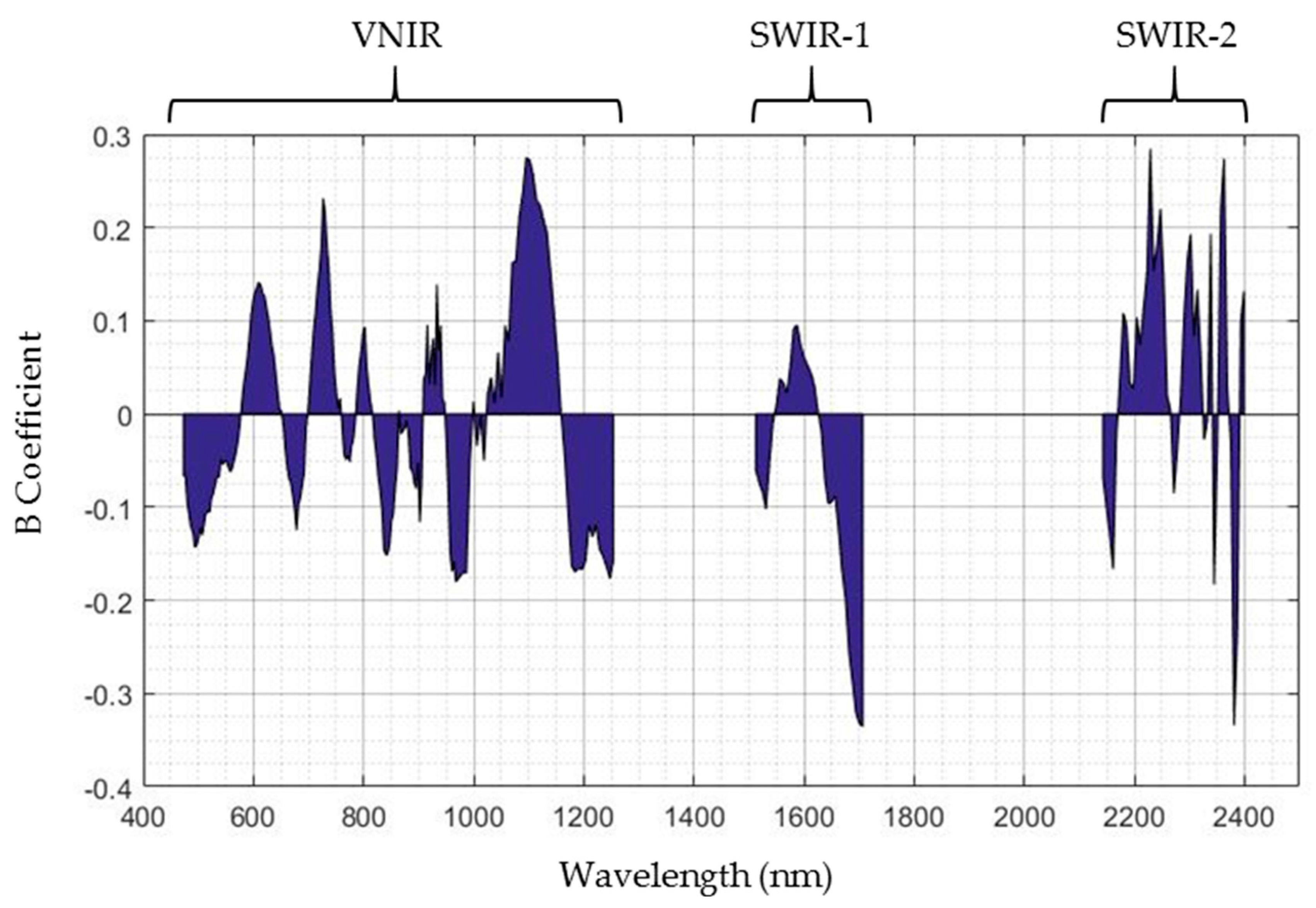
Figure 6.
Roads predicted friction map of the study site.


Table 1.
Optical properties of the AisaFenix 1K hyperspectral imaging spectrometer.
| Optical Properties | VNIR | SWIR |
|---|---|---|
| Detector Type | CMOS | MCT |
| Spectral Range | 380–970 nm | 970–2500 nm |
| Spectral Resolution | ≤4.5 nm | ≤12 nm |
| Spectral Pixels | 348 | 246 |
| Spatial Pixels | 1024 | 1024 |
| F-Number | 2.4 | |
| FOV | 40° | |
| IFOV | 0.039° | |
Table 2.
Sample groups by friction value with ranks.
| Group Rank | Minimum | Maximum | n | Color Code 1 |
|---|---|---|---|---|
| A | 0.077 | 0.383 | 272 | Red |
| B | 0.383 | 0.522 | 276 | Magenta |
| C | 0.522 | 0.593 | 274 | Green |
| D | 0.593 | 0.664 | 274 | Blue |
| E | 0.664 | 0.796 | 274 | Black |
1 Color code used in Figure 2 representing the group ranks.
Table 3.
Possible spectral assignments.
| Feature ID | Wavelength (nm) | Sign Indication | Possible Assignment |
|---|---|---|---|
| 1 | 726 | Positive | Metal Oxides/Surface Texture |
| 2 | 1095 | Positive | Hygroscopic Water |
| 3 | 1706 | Negative | Organic Compounds/Polymers |
| 4 | 2229 | Positive | Clay Minerals |
| 5 | 2340 | Positive | Calcium Carbonate |
| 6 | 2381 | Negative | Organic Compounds/Polymers |
© 2018 by the authors. Licensee MDPI, Basel, Switzerland. This article is an open access article distributed under the terms and conditions of the Creative Commons Attribution (CC BY) license (http://creativecommons.org/licenses/by/4.0/).
Share and Cite
MDPI and ACS Style
Carmon, N.; Ben-Dor, E. Mapping Asphaltic Roads’ Skid Resistance Using Imaging Spectroscopy. Remote Sens. 2018, 10, 430. https://doi.org/10.3390/rs10030430
AMA Style
Carmon N, Ben-Dor E. Mapping Asphaltic Roads’ Skid Resistance Using Imaging Spectroscopy. Remote Sensing. 2018; 10(3):430. https://doi.org/10.3390/rs10030430
Chicago/Turabian StyleCarmon, Nimrod, and Eyal Ben-Dor. 2018. "Mapping Asphaltic Roads’ Skid Resistance Using Imaging Spectroscopy" Remote Sensing 10, no. 3: 430. https://doi.org/10.3390/rs10030430
Note that from the first issue of 2016, this journal uses article numbers instead of page numbers. See further details here.