High Turbidity Solis Clear Sky Model: Development and Validation

Abstract

The Solis clear sky model is a spectral scheme based on radiative transfer calculations and the Lambert–Beer relation. Its broadband version is a simplified fast analytical version; it is limited to broadband aerosol optical depths lower than 0.45, which is a weakness when applied in countries with very high turbidity such as China or India. In order to extend the use of the original simplified version of the model for high turbidity values, we developed a new version of the broadband Solis model based on radiative transfer calculations, valid for turbidity values up to 7, for the three components, global, beam, and diffuse, and for the four aerosol types defined by Shettle and Fenn. A validation of low turbidity data acquired in Geneva shows slightly better results than the previous version. On data acquired at sites presenting higher turbidity data, the bias stays within ±4% for the beam and the global irradiances, and the standard deviation around 5% for clean and stable condition data and around 12% for questionable data and variable sky conditions.

1. Introduction

Anthropogenic activities have become an important factor in climate change and continuous monitoring of the solar irradiance reaching the ground is essential to understand the impact of such changes on the environment. Unfortunately, the density of the ground measurement network is insufficient, especially on continents like Africa or Asia. To circumvent this lack of measured data, meteorological satellites are of great help and models converting the satellite images into the different radiation components are becoming increasingly useful.

The first step in evaluating the solar irradiance from satellite images is a good knowledge of the highest possible radiation transmitted by a cloudless atmosphere. This can be done with the help of clear sky model taking into account the aerosol and water vapor content of the atmosphere. Multiple clear sky models can be found in the literature, but none of them is able to evaluate solar radiation for high turbidities resulting from heating and transportation activities and encountered in countries like India or China. For example, the Gueymard CPCR2 model [1] is limited to β turbidity values lower than 0.4 (which correspond to an aerosol optical depth at 700 nm aod₇₀₀ of 0.64 for rural aerosol type, Angström exponent α = 1.3), Gueymard REST2 [2] is limited to β = 1 (aod₇₀₀ = 1.6, rural aerosol), Bird’s model [3] is defined for visibility values up to 23 km (which corresponds to an aod₇₀₀ = 0.27), and the ESRA clear sky scheme [4,5,6] was developed for Linke turbidity values T_L [7] not exceeding a value of 7 (i.e., an aerosol optical depth aod₇₀₀ = 0.44 for a 2 cm water vapor column w).

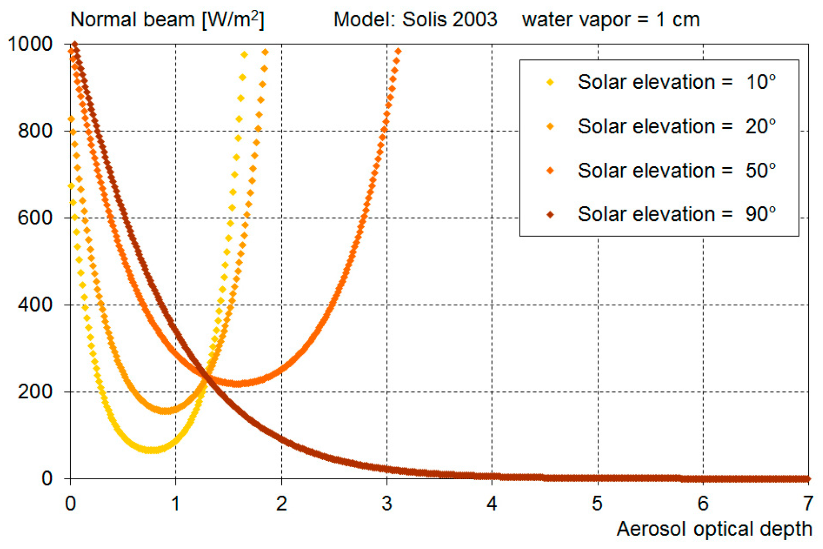
The spectral Solis clear sky scheme was first developed within the Mesor European program, whose subject was the management and exploitation of solar resource knowledge. Due to the spatial and temporal range of the satellite images, the on line process to evaluate irradiance maps implies fast analytical models. In [8], Ineichen published a broadband fast analytical version of the Solis model for rural aerosol type, and in 2010 a version in the form of an Excel tool for the four types of aerosols was defined by Shettle and Fenn [9] and Shettle [10]. These versions were limited to broadband aerosol optical depth values aod₇₀₀ lower than 0.45; they diverge for higher turbidity, as shown by Zhang [11]. This is illustrated in Figure 1, where the normal beam irradiance I_bn is represented versus the aerosol optical depth for the Solis 2008 model and different solar elevation angles.

This paper presents the development and validation of a new version of the analytical Solis scheme valid for the three radiation components, the global, the beam, and the diffuse, and the four aerosol types, urban, rural, maritime, and tropospheric.

2. Basis of the Solis Scheme

The original Solis clear sky model [12] was first developed within the European program Joule in 2004 in the frame of the Heliosat project, whose aim was to derive and assess the evaluation of the solar irradiance components from the geostationary meteorological satellite MSG (Meteosat Second Generation). The scheme is based on the spectral Radiative Transfer Model (RTM) LibRadTran [13,14] and the Lambert–Beer attenuation relationship:

$$I_{bn}=I_o·{\mathrm{e}}^{-M\mathsf{\tau }},$$

(1)

where I_o is the extraterrestrial irradiance, I_bn the normal beam irradiance reaching the ground, M the optical air mass, and τ the extinction coefficient. In order to adapt this relation to broadband irradiance, it has to be modified slightly. Three distinct extinction coefficients, one for each of the irradiance components, are defined, as well as three exponent coefficients in the Lambert–Beer attenuation relation. The diffuse irradiance is the result of the scattering process of the beam component during its crossing of the atmosphere. In order to minimize the number of coefficients, a common modified extraterrestrial irradiance I_o′ expressed in W/m² is defined.

The three broadband relations then take the following form:

$$I_{bn}=I_o{}^{\prime }·e^{\left(-{\tau }_b/{\sin }^{b}h\right)} I_{gh}=I_o{}^{\prime }·e^{\left(-{\tau }_g/{\sin }^{g}h\right)}·\sin h{I}_{dh}=I_o{}^{\prime }·e^{\left(-{\tau }_d/{\sin }^{d}h\right)},$$

(2)

where I_bn, I_gh and I_dh represent the normal beam irradiance, the horizontal global, and the horizontal diffuse components, respectively, and h is the solar elevation angle.

The model is then driven by seven parameters: the modified extraterrestrial irradiance I_o′, the three extinction coefficients τ_b, τ_g and τ_d for the beam, global, and diffuse irradiance, respectively, and b, g, and d are the corresponding sine exponent coefficients.

The justification of these equations can be found in [1,12].

3. Solis Extension to High Turbidity

To circumvent the limitation of the previous Solis scheme, we developed a new version that is applicable for aerosol optical depth values aod up to 7. This large range of turbidity values is needed to avoid unrealistic irradiance values resulting from extreme input parameters to automatic processes. However, one has to keep in mind that above aod = 2, it is not clear that the turbidity can be considered an aerosol optical depth, but a “turbidity” due to bigger particles like sand, or thin, high-altitude clouds. Nevertheless, it is important that in on line automatic production processes, the model does not diverge and still derives coherent values, even with some discrepancies from ground measurements.

3.1. Model Development

The main parameters driving the determination of the solar radiation reaching the ground for a cloudless atmosphere are the aerosol optical depth aod, the total atmospheric precipitable water vapor column w expressed in centimeters, the altitude of the considered site, and the aerosol type. Other atmospheric content such as O₃, NO_x, etc. have a very low influence of the atmospheric transmittivity and will be considered constant in the development of the model.

In the first step, we made spectral calculations with LibRadTran for each combination of the following parameters.

These RTM calculations permit us to generate the seven coefficients that drive the model: I_o’, τ_b, b, τ_g, g, τ_d, and d. The next step is to develop an analytical formulation for these coefficients with the four input parameters given in

Table 1. Aerosol types, altitudes, optical depths aod₅₅₀, and water vapor columns w values for the RTM calculations with LibRadTran.

Aerosol Type	Altitude	Aod550	W
urban	sea level	0.01	0.01
rural	500 m	0.03	0.03
maritim	1000 m	0.05	0.05
tropospheric	2000 m	0.1	1
	3000 m	0.15	0.15
	4000 m	0.2	0.2
	5000 m	0.4	0.3
	6000 m	0.7	0.5
	7000 m	1	1
		1.5	1.5
		2	2
		3	3
		4	4
		5	6
		6	8
		7	10

.

The analysis of I_o′, τ_b, τ_g dependence with the aod shows a similar behavior for these three parameters. A third-order polynomial model of the form is applicable:

$$\begin{gathered} I_o{}^{\prime }/I_o=a_i·ao{d}^3+b_i·ao{d}^2+c_i·aod+d_i \\ {\tau }_b=a_b·ao{d}^3+b_b·ao{d}^2+c_b·aod+d_b \\ {\tau }_g=a_g·ao{d}^3+b_g·ao{d}^2+c_g·aod+d_g. \end{gathered}$$

(3)

The behavior of I_o′/I_o and τ_g is represented in Figure 2.

We then analyzed the dependence of each of the a, b, c and d coefficients with the atmospheric water vapor content w. The behavior of the four coefficients shows a common dependence of the form:

$$n=n_1·w^{0.5}+n_2·\ln w+n_3,$$

(4)

where n replaces the a, b, c, and d coefficients for I_o′, τ_b and τ_g.

The best fit for these coefficients is illustrated in Figure 3.

Finally, the dependence of the three above coefficients on the altitude and the normalized atmospheric pressure p/p_o (the pressure p at a given altitude normalized by the corresponding sea level pressure p_o) is analyzed. It appears that a linear regression gives good results.

The model has the following form (for a_i, b_i, c_i, d_i, a_b, b_b, c_b, d_b, a_g, b_g, c_g, and d_g):

$$\begin{gathered} a=a_1·w^{0.5}+a_2·\ln w+a_3 \\ b=b_1·w^{0.5}+b_2·\ln w+b_3 \\ c=c_1·w^{0.5}+c_2·\ln w+c_3 \\ d=d_1·w^{0.5}+d_2·\ln w+d_3 \end{gathered}$$

(5)

and the general form n_i of a, b, c and d coefficient is obtained by a linear function of p/p_o:

$$n_i=n_{\mathrm{i}1}·p/p_o+n_{\mathrm{i}2}.$$

(6)

Finally, the inputs for the model for I_o′/I_o, τ_b, and τ_g, consist of the aerosol optical depth at 550 nm, aod₅₅₀; the water vapor content of the atmosphere, w; and the relative atmospheric pressure, p/p_o. The corresponding coefficients are given in a 4 × 3 × 2 matrix (see Appendix A).

For τ_d, the best correlation we found is a relation with τ_b and τ_g that has the form:

$${\tau }_d=c_{td1}+c_{td2}·{\tau }_g+c_{td3}/{\tau }_b+c_{td4}·{\tau }_g{}^2+c_{td5}/{\tau }_b{}^2+c_{td6}·{\tau }_g/{\tau }_b.$$

(7)

The exponents of sin h in the Lambert–Beer function are best fitted as follows:

$$\begin{gathered} g=c{a}_1+c{a}_2·\ln w+c{a}_3·\ln aod+c{a}_4{\ln }^{2}w+c{a}_5·{\ln }^{2}aod+c{a}_6·\ln w·\ln aod \\ b=c{b}_1+c{b}_2·w+c{b}_3·aod \\ d=c{d}_1+c{d}_2·\ln w+c{d}_3·aod+c{d}_4·ao{d}^2+c{d}_5·ao{d}^3+c{d}_6·ao{d}^4+c{d}_7·ao{d}^5. \end{gathered}$$

(8)

All coefficients for the four aerosol types are given in Appendix A, as well as in the form of an Excel tool [15].

3.2. Solis Analytical Model Versus RTM Calculated Parameter Comparison

The comparison of the seven parameters of the model is expressed as scatter plots between the Solis analytical model parameters and the corresponding LibRadTran calculated parameters. The validation points should be aligned on the 1:1 diagonal. On the graphs are also given the average parameter value, the mean bias difference mbd, the standard deviation sd and the correlation coefficient R². An illustration is given in Figure 4 for I_o′ and the g coefficient.

The average mbd and sd values cannot be taken as an absolute validation of the precision as all the values calculated from the input matrix (altitude, aod, and w) have the same weight. Nevertheless, it gives a good idea of the roughness of the parameter best fit. These values are given in

Table 2. Average, mbd, sd and R² for the I_o′, τ_b, b, τ_g, g, τ_d, and d model.

	Io'				τg				a
aerosol type	average	mbd	sd	R2	average	mbd	sd	R2	average	mbd	sd	R2
rural	6284	0	93	0.998	−1.49	0.00	0.01	1.000	0.41	0.00	0.02	0.993
urban	6036	0	95	0.997	−1.68	0.00	0.02	1.000	0.44	0.00	0.02	0.991
tropospheric	5380	0	40	0.999	−1.40	0.00	0.01	1.000	0.41	0.00	0.02	0.992
maritime	12,210	−8	134	0.998	−1.69	0.00	0.01	1.000	0.39	0.00	0.02	0.994
					τb				b
rural					−2.21	0.00	0.01	1.000	0.42	0.00	0.02	0.965
urban					−2.21	0.00	0.01	1.000	0.44	0.00	0.03	0.941
tropospheric					−2.08	0.00	0.01	1.000	0.40	0.00	0.02	0.976
maritime					−2.68	0.00	0.01	1.000	0.45	0.00	0.02	0.912
					τd				c
rural					−2.75	0.01	0.04	0.998	0.32	0.00	0.01	0.995
urban					−3.08	0.01	0.05	0.999	0.29	0.00	0.01	0.995
tropospheric					−2.67	0.01	0.04	0.998	0.33	0.00	0.01	0.995
maritime					−2.86	0.01	0.04	0.999	0.31	0.00	0.01	0.995

.

3.3. Modeled versus RTM Calculated Irradiance Comparison

In the same way, the modeled irradiances are compared to the corresponding irradiances estimated from the coefficients calculated with LibRadTran. The validation is expressed as scatter plots and the usual first-order statistics. Here, again due to the unweighted input matrix, the validation values obtained do not give absolute precision. The scatter plots given in Figure 5 illustrate the behavior of the model. They represent the modeled values plotted against the corresponding values evaluated from RTM calculations, for the three components and urban type aerosols.

To obtain the diffuse component, there are two possibilities: the use of the model coefficients I′_o, τ_d and d, or to evaluate it from the global and the beam components with the use of the closure equation I_dh = I_gh – I_bn · sin h. The diffuse component obtained from the closure equation looks slightly better in Figure 4, but it presents negative values for very low solar elevations.

The comparison statistics are given in

Table 3. Average, mbd, sd, and R² for the irradiance components.

	Igh				Ibn				Idh
aerosol type	average	mbd	sd	R2	average	mbd	sd	R2	average	mbd	sd	R2
rural	727	0	4	1.000	549	0	5	1.000	223	0	7	0.998
urban	632	0	7	1.000	543	0	3	1.000	167	0	7	0.997
tropospheric	740	0	5	1.000	559	0	7	1.000	227	0	7	0.999
maritime	753	−1	17	0.997	519	−3	18	0.999	266	2	11	0.998

.

All the development and validation graphs for the rural aerosol type are given in Appendix B.

4. Model Validation against Ground Measurements

The first step in the model validation process is to apply stringent quality control to the collected ground data. Then, only data acquired under clear sky conditions should be selected; the validation is then applied on these data and the validity of the model is quantified using classical first-order statistical indicators: the mean bias difference (mbd) and the standard deviation (sd).

4.1. Quality Control of the Ground Data

The validity of the results obtained from the use of measured data is highly correlated to the quality of the data bank used as a reference. Controlling data quality is therefore the first step in the process of validating models against ground data. This should be done properly during the acquisition process and automated in order to rapidly detect significant instrumental problems like sensor failure, errors in calibration, orientation, leveling, tracking, consistency, etc. Normally, this quality control process should be done by the institution responsible for the measurements. Unfortunately, this is not always the case. Even if some quality control procedures have been implemented, they might not be sufficient to catch all errors, or the data points might not be flagged to indicate the source of the problem. A stringent control quality procedure must therefore be adopted in the present context, and its various elements are given in what follows.

If the three solar irradiance components, beam, diffuse, and global, are available, a consistency test can be applied, based on the closure equation that links them:

$$I_{gh}=I_{dh}+I_{bn}·\sin h.$$

(9)

A posteriori automatic quality control cannot detect all acquisition problems, however. The remaining elements to be assessed are threefold:

• The measurement’s time stamp (needed to compute the solar geometry);
• The sensors’ calibration coefficient used to convert the acquired data into physical values;
• The coherence between the parameters.

It has to be noted that, for the data of Solar Village, even if the closure equation satisfies the selection conditions, as can be seen in Figure 6, a clear pattern appears due to calibration differences of up to 6–8% between the winter months and the summer months. The bias between the beam irradiance measurements and the closure equation values are negative in the summer months; it is not clear what the source of the difference is. This can be an issue of the temperature and/or solar altitude dependence of the sensors; it is difficult to find out a posteriori what component is questionable and why.

A complete description of the quality control procedure is given by Ineichen [16].

4.2. Clear Conditions Selection

To perform the selection, the criteria defined in Ineichen [17] are applied:

• If three components are available, the closure equation must be satisfied within −50 W/m² − 5% and +50 W/m² + 5%; if only two components are available, all the values are kept.
• The modified global clearness K_t′ (as defined by Perez et al. in [18]) of the measurements is higher than 0.65.
• The stability of the global clearness index ΔK_t′ is better than 0.01 (ΔK_t′ is evaluated by the difference of the considered hour and the average of the considered hour, the preceding one, and the following one)

This selection minimizes the cloud contamination. It is restrictive, but for the purposes of the comparison, it ensures that only clear and stable conditions are selected. It shows its importance particularly with data from Xianghe, where often the beam component is very low or missing in the middle of the day, while the corresponding global component shows clear conditions (due to saturation?). This is illustrated in Figure 7.

4.3. Statistical Indicators and Graphical Representation

The comparison is done on an hourly basis, the model–measurements difference is computed, so that a positive value of the mean bias difference represents an overestimation of the model. The following indicators are used to quantify model performance:

• First-order statistics for a given site: the mean bias difference (mbd) and the standard deviation (sd). In addition, qualitative visualization is made with the help of model versus measurement scatterplots.
• The seasonal dependence of the bias and its dependence with the aerosol optical depth (aod);
• The frequency distribution of the model–measurements differences and the corresponding cumulated frequencies.

4.4. Ground Measurements for the Validation

To assess the validity of the model for low turbidity values, we first made a validation of the same data as in [18] acquired in Geneva for the years 2004 to 2011, where the aod is pretty low.

The average aerosol optical depth in Geneva is on the order of 0.17, with a maximum of 0.5 during polluted episodes. As no specific aerosol optical depth values are measured in Geneva, we used one of the best state-of-the-art models, REST2 [5], to retrieve by retrofit the aod following the method described in [19].

The next validation step is to do a comparison with ground data acquired at a site with higher turbidity values. To conduct the validation, sites that jointly acquire the irradiance components and the aerosol optical depth are needed. They are very scarce, so that not all conditions could be analyzed. Irradiance data from three Baseline Surface Radiation Network (BSRN) sites and from one Indian National Institute of Wind Energy (NIWE) site are used for the validation. The aerosol optical depths are retrieved from the Aerosol Robotic Network (AERONET). The latitude, longitude, altitude, networks, and acquired parameters are given in

Table 4. Latitude, longitude, altitude, networks, and acquired parameters for the considered sites.

Site	Network	Latitude	Longitude	Altitude	Global	Beam	Diffuse	Ta	Hr	Aod
Ilorin	BSRN/AERONET	8.53	4.57	350	x		x	x	x	x
Jaipur	NIWE/AERONET	26.81	75.86	403	x	x	x	x	x	x
Solar Village	BSRN/AERONET	24.91	46.41	650	x	x	x	x	x	x
Xianghe	BSRN/AERONET	39.75	116.69	22	x	x	x			x

.

The median values of the aod for the four sites are situated between 0.3 and 0.55, with maximum values around 1.5 to 4. The cumulated frequencies of occurrence of the aerosol optical depth and the atmospheric water vapor content are given in Figure 8.

5. Validation Results and Discussion

The results of the validation against the ground data acquired in Geneva are illustrated in Figure 9 for the normal beam and the global horizontal irradiance. Done on the same dataset as in [17], it shows that the first-order statistics are slightly better than for the previous version of Solis.

The first-order statistics of the model validation against data acquired at high turbidity sites are given in

Table 5. First-order statistics for the four sites and rural aerosol type. The irradiance is expressed in (W·h/m²·h) and the irradiation in (kWh/m²·day).

	Hourly Values
Site	Normal Beam				Horizontal Global			Horizontal Diffuse
	nb	Average	mbd	sd	Average	mbd	sd	Average	mbd	sd
Ilorin 1998–2005	289	646	−2%	12%	845	1%	5%	277	2%	22%
Jaipur 2016–2017	387	670	4%	5%	715	3%	3%	198	4%	13%
Solar Village 1999–2002	3198	790	−2%	5%	784	−1%	4%	165	4%	19%
Xianghe 2008–2015	1161	762	−2%	13%	612	−5%	6%	132	−10%	33%
	"daily values"
	nb	average	mbd	sd	average	mbd	sd	average	mbd	sd
Ilorin 1998–2005	39	2.3	0%	8%	3.0	1%	4%	0.9	−1%	20%
Jaipur 2016–2017	69	3.6	4%	4%	3.8	3%	2%	1.0	5%	10%
Solar Village 1999–2002	453	5.5	−2%	3%	5.5	−1%	3%	1.2	4%	12%
Xianghe 2008–2015	178	4.9	−2%	14%	3.9	−5%	6%	0.8	−10%	33%

for the rural aerosol type, and in

Table 6. First-order statistics for the four sites and urban aerosol type. The irradiance is expressed in (W·h/m²·h) and the irradiation in (kWh/m²·day).

	Hourly Values
Site	Normal Beam				Horizontal Global			Horizontal Diffuse
	nb	Average	Mbd	Sd	Average	Mbd	Sd	Average	Mbd	Sd
Ilorin 1998—2005	289	646	−3%	12%	845	−8%	7%	277	−20%	20%
Jaipur 2016—2017	387	670	3%	6%	715	−4%	4%	198	−16%	11%
Solar Village	3198	790	−3%	5%	784	−5%	4%	165	−14%	19%
Xianghe 2008—2015	1161	762	−2%	13%	612	−8%	8%	132	−24%	30%
	Daily Values
	nb	Average	Mbd	sd	Average	Mbd	Sd	Average	Mbd	Sd
Ilorin 1998—2005	39	2.3	−2%	9%	3.0	−7%	6%	0.9	−22%	19%
Jaipur 2016—2017	69	3.6	3%	4%	3.8	−3%	3%	1.0	−15%	8%
Solar Village	453	5.5	−3%	3%	5.5	−5%	3%	1.2	−13%	13%
Xianghe 2008—2015	178	4.9	−2%	14%	3.9	−8%	9%	0.8	−24%	26%

for the urban aerosol type. The tables report the number of nb values kept for the validation, the average measured irradiance and irradiation, the relative mean bias difference, mbd, and the standard deviation, sd. Results are provided for the three irradiance components and for all sites. Due to the different climates and quality of the data, the number of selected data can be very different from one site to the other.

The main results drawn from the table are the following:

• For all sites, choosing the rural aerosol type gives the best results in terms of mean bias and standard deviation, especially for the global component.
• For Ilorin, the high standard deviation is due to the high variability of the sky conditions; it can also be a result of the beam retrieval from the global and the diffuse components. For Xianghe, the poor quality of the data induces this higher standard deviation.
• The Jaipur and Solar Village datasets show the overall best results in term of mean bias and standard deviation.
• The “daily values” represent the sum of only the hourly values kept for the validation: it is not the daily integral (the sum of all the values of the day). This is particularly the case during partially cloudy days where only a few hourly values are acquired during cloudless conditions. The consequence is that, for example, at Ilorin, where the sky conditions are highly variable and clear days from sunrise to sunset are very scarce, the average “daily value” is low.

A deeper analysis of the results leads to the following general observations:

• Ground measurements and modeled values can be represented on the same graph in different colors. If the model faithfully reproduces the measurements, the envelopes of the data clouds should be similar. This is illustrated for the site of Solar Village in Figure 10 where the beam clearness index is plotted against the global clearness index on the left graph (a) and the diffuse fraction against the global clearness index on the right graph (b); the measurements are represented in green and the modeled values in blue.
• The trends of the bias as a function of the aerosol optical depth show no particular pattern for all the sites, except for Xianghe, where a non-significant trend is due to the dispersion. These dependences are illustrated in Figure 11 in hourly values, for the site of Solar Village and rural aerosol type.
• The seasonal dependence of the bias for both the global and the beam irradiance components shows no significant pattern. An illustration is given in Figure 12 for data from Solar Village in hourly values.
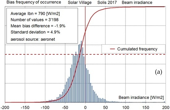
• With the exception of the site of Ilorin, the distributions of the bias around the 1:1 model–measurements axis are near normal; for this reason, the first-order statistics represented by the mean bias and the standard deviation can be considered reliable. An example is given in Figure 13 for the site of Solar Village. The figure displays the hourly bias frequency distribution for both I_bn and I_gh irradiance components. The cumulated frequencies (red curve) are also represented in the graphs.

6. Conclusions

When dealing with satellite images to derive the irradiance components worldwide and every 15 min, the calculation time should be as short as possible. The analytical Solis clear sky scheme was developed to fulfill this requirement but had the weakness of being limited to aerosol optical depth values lower than 0.45. The new analytical Solis scheme is valid for aod₅₅₀ values up to seven, even if very high values are not realistic as an optical depth; it is probably due to bigger particles like sand, or thin, high-altitude clouds. Nevertheless, in contrary to other clear sky models, this permits us to produce coherent irradiance values, even with questionable input data. Indeed, for example, the aod, due to the difficulty of retrieving it by automatic processes, can take on out-of-range or unrealistic values.

The new Solis clear sky scheme is developed for aerosol optical depths values aod₅₅₀ from 0.02 to 7, for atmospheric water vapor w content from 0.01 to 10 cm, for altitude from sea level to 7000 m, and for four aerosol types, as defined by Shettle and Fenn [2]. For the urban, rural, and tropospheric aerosol types, the validation against the original LibRadTran RTM calculations presents no bias and a standard deviation lower than 1% for the global and the beam component, and 3% for the diffuse. When dealing with maritime aerosol type, the standard deviation is 2.2%, 3.4%, and 4%, respectively, for the global, the beam, and the diffuse components.

The validation against ground measurements acquired in Geneva, Ilorin, Jaipur, Solar Village, and Xianghe gives a mean bias difference less than ±4%, a standard deviation of 3–6% for the global component, and a mean bias difference less than ±3% with a standard deviation of 5–13% for the beam component. The 12–13% standard deviations are due to either the high variability of the sky conditions or the poor quality of the ground data.

As it is very difficult to find ground measurements covering the complete range of validity of the new Solis analytical scheme, it cannot be completely validated. However, the new version faithfully reproduces the RTM LibRadTran calculations.

References

- Gueymard, C. A two-band model for the calculation of clear Sky Solar Irradiance, Illuminance, and Photosynthetically Active Radiation at the Earth Surface. Sol. Energy 1989, 43, 253–265. [Google Scholar] [CrossRef]
- Gueymard, C. Direct solar transmittance and irradiance predictions with broadband models. Part 1: Detailed theoretical performance assessment. Sol. Energy 2003, 74, 355–379. [Google Scholar] [CrossRef]
- Bird, R.E.; Huldstrom, R.L. Direct insolation models. Trans. ASME J. Sol. Energy Eng. 1980, 103, 182–192. [Google Scholar] [CrossRef]
- Wald, L. European Solar Radiation Atlas; Commission of the European Communities Presses de l’Ecole, Ecole des Mines de Paris: Paris, France, 2000. [Google Scholar]
- Rigollier, C.; Bauer, O.; Wald, L. On the Clear Sky Model of the ESRA—European Solar Radiation Atlas—With Respect to the Heliosat Method. Sol. Energy 2000, 68, 33–48. [Google Scholar] [CrossRef]
- Geiger, M.; Diabaté, L.; Ménard, L.; Wald, L. A web Service for Controlling the Quality of Measurements of Global Solar Irradiation. Sol. Energy 2002, 73, 475–480. [Google Scholar] [CrossRef]
- Linke, F. Transmissions-Koeffizient und Trübungsfaktor. Beiträge zur Physik der freien Atmosphäre 1992, 10, 91–103. [Google Scholar]
- Ineichen, P. A broadband simplified version of the Solis clear sky model. Sol. Energy 2008, 82, 758–762. [Google Scholar] [CrossRef]
- Shettle, E.P.; Fenn, R.W. Models Fort the Aerosol of Lower Atmosphere and the Effect of Humidity Variations on Their Optical Properties. 1979. Available online: http://www.dtic.mil/docs/citations/ADA085951 (accessed on 2 March 2018).
- Shettle, E.P. Models of aerosols, clouds and precipitation for atmospheric propagation studies. In Proceedings of the AGARD, Atmospheric Propagation in the UV, Visible, IR, and MM-Wave Region and Related Systems Aspects Conference, Copenhagen, Denmark, 9–13 October 1989. [Google Scholar]
- Zhang, T.; Stackhouse, P.W., Jr.; Chandler, W.S.; Westberg, D.J. Application of a global-to-beam irradiance model to the NASA GEWEX SRB dataset: An extension of the NASA Surface meteorology and Solar Energy datasets. Sol. Energy 2014, 110, 117–131. [Google Scholar] [CrossRef]
- Mueller, R.W.; Dagestad, K.F.; Ineichen, P.; Schroedter-Homscheidt, M.; Cros, S.; Dumortier, D.; Kuhlemann, R.; Olseth, J.A.; Piernavieja, G.; Reise, C.; et al. Rethinking satellite based solar irradiance modelling—The SOLIS clear-sky module. Remote Sens. Environ. 2004, 91, 160–174. [Google Scholar] [CrossRef]
- Mayer, B.; Kylling, A. Technical note: The libRadtran software package for radiative transfer calculations—Description and examples of use. Atmos. Phys. 2005, 5, 1855–1877. [Google Scholar] [CrossRef]
- Mayer, B.; Kylling, A.; Emde, C.; Buras, R.; Hamann, U. LibRadTran: Library for Radiative Transfer Calculations, Edition 1.0 for Libradtran Version 1.5-beta. 2010. Available online: https://clouds.eos.ubc.ca/~phil/courses/eosc582_2010/textfiles/libRadtran.pdf (accessed on 3 March 2018).
- Ineichen, P. Solis 2017 Excel Tool. Password: Solis2017. Available online: http://www.adpi.ch/Solis2017/Solis2017-tool.xlsx (accessed on 28 February 2017).
- Ineichen, P. Satellite Irradiance Based on MACC Aerosols: Helioclim 4 and SolarGIS, Global and Beam Components Validation. In Proceedings of the EuroSun 2014, Aix-les-Bains, France, 16–19 Septembre 2014. [Google Scholar]
- Ineichen, P.; Barroso, C.S.; Geiger, B.; Hollmann, R.; Marsouin, A.; Mueller, R. Satellite Application Facilities irradiance products: hourly time step comparison and validation over Europe. Int. J. Remote Sens. 2009, 30, 5549–5571. [Google Scholar] [CrossRef]
- Perez, R.; Ineichen, P.; Seals, R.; Zelenka, A. Making full use of the clearness index for parameterizing hourly insolation conditions. Sol. Energy 1990, 45, 111–114. [Google Scholar] [CrossRef]
- Ineichen, P. Validation of models that estimate the clear sky global and beam solar irradiance. Sol. Energy 2016, 132, 332–344. [Google Scholar] [CrossRef]
Figure 1.
Behavior of the normal beam irradiance with the aerosol optical depth for the 2008 Solis version and different solar elevation angles.
Figure 2.
Behavior of the enhanced solar constant Io′/Io (a) and the extinction coefficient τ (b) with the spectral aerosol optical depth at 550 nm.
Figure 3.
Behavior of the cubic equation coefficients a, b, c and d, respectively graph (a–d), with the water vapor column w.
Figure 4.
Modeled Io′ coefficient (a) and modeled g coefficient (b) versus the corresponding RTM calculated value.
Figure 5.
Modeled against RTM calculated irradiance comparison for the beam (a), the global (b), the diffuse (c), and the closure diffuse (d) components.
Figure 6.
Illustration of the calibration uncertainty for the site of Solar Village.
Figure 7.
Illustration of the questionable data for the site of Xianghe.
Figure 8.
Cumulated frequency of occurrence of the aerosol optical depth (a) and the atmospheric water vapor content (b) for the four sites.
Figure 9.
Validation against ground data acquired in Geneva for the beam irradiance (a) and the global component (b). The aod is retrofitted with REST2. For comparison, the same graphs are given for the previous version of Solis (c,d).
Figure 10.
Beam clearness index (a) and diffuse fraction (b) versus the global clearness index.
Figure 11.
Bias versus the aerosol optical depth for normal beam irradiance (a) and global irradiance (b) for the site of Solar Village.
Figure 12.
Seasonal dependence of the bias for the normal beam irradiance (a) and the global irradiance (b) irradiance components for the site of Solar Village.
Figure 13.
Frequency of occurrence of the bias around the 1:1 axis for the beam (a) and the global (b) irradiance components.