Optimisation of Savannah Land Cover Characterisation with Optical and SAR Data


1
School of Science and the Environment, Manchester Metropolitan University, Manchester M15GD, UK
2
Geography Department, Humboldt-Universität zu Berlin, Unter den Linden 6, 10099 Berlin, Germany
*
Author to whom correspondence should be addressed.
Remote Sens. 2018, 10(4), 499; https://doi.org/10.3390/rs10040499
Submission received: 28 January 2018
/
Revised: 12 March 2018
/
Accepted: 18 March 2018
/
Published: 22 March 2018
(This article belongs to the Section Remote Sensing Image Processing)
Abstract
:Accurately mapping savannah land cover at the regional scale can provide useful input to policy decision making efforts regarding, for example, bush control or overgrazing, as well as to global carbon emissions models. Recent attempts have employed Earth observation data, either from optical or radar sensors, and most commonly from the dry season when the spectral difference between woody vegetation, crops and grasses is maximised. By far the most common practice has been the use of Landsat optical bands, but some studies have also used vegetation indices or SAR data. However, conflicting reports with regards to the effectiveness of the different approaches have emerged, leaving the respective land cover mapping community with unclear methodological pathways to follow. We address this issue by employing Landsat and Advanced Land Observing Satellite Phased Array type L-band Synthetic Aperture Radar (ALOS PALSAR) data to assess the accuracy of mapping the main savannah land cover types of woody vegetation, grassland, cropland and non-vegetated land. The study area is in southern Africa, covering approximately 44,000 km2. We test the performance of 15 different models comprised of combinations of optical and radar data from the dry and wet seasons. Our results show that a number of models perform well and very similarly. The highest overall accuracy is achieved by the model that incorporates both optical and synthetic-aperture radar (SAR) data from both dry and wet seasons with an overall accuracy of 91.1% (±1.7%): this is almost a 10% improvement from using only the dry season Landsat data (81.7 ± 2.3%). The SAR-only models were capable of mapping woody cover effectively, achieving similar or lower omission and commission errors than the optical models, but other classes were detected with lower accuracies. Our main conclusion is that the combination of metrics from different sensors and seasons improves results and should be the preferred methodological pathway for accurate savannah land cover mapping, especially now with the availability of Sentinel-1 and Sentinel-2 data. Our findings can provide much needed assistance to land cover monitoring efforts to savannahs in general, and in particular to southern African savannahs, where a number of land cover change processes have been related with the observed land degradation in the region.

1. Introduction
Savannahs are important ecosystems that are found on almost half of the African continent and a fifth of the Earth’s surface [1]. They consist of different densities of grasses and woody vegetation and are host to a number of ongoing land system science debates, such as equilibrium dynamics [2], the role of anthropogenic processes in land degradation [3] and the contribution of drylands to the global carbon cycle [4]. Savannah biomes provide a plethora of ecosystem resources and services, and play an important role in numerous processes, both natural and anthropogenic, such as biomass production, the timing and characteristics of fire, the cycling of nutrients, surface runoff and soil erosion, wind erosion, carbon sequestration, etc. [4,5,6,7]
Unfortunately, African savannahs undergo massive conversions and are affected by land degradation and desertification processes [8], leading to a decline in the ecosystem services provided to some of the continent’s poorest and most vulnerable human populations [9,10]. Reductions in the productivity of dryland savannahs have major social and political implications [11], and given their importance, the United Nations (UN) has labelled the accurate quantification of savannah degradation as of high priority [12].
Mapping the extent of the main constituents of savannah land cover is, therefore, essential to regional efforts to protect and manage savannahs. At large scales, the use of Earth observation (EO) technologies is the only viable approach [13,14]. Most EO studies aiming to map and monitor large scale land cover have employed optical Landsat data, due to the appropriateness of the spatial resolution as well as to the freely available 40-year long archive [15,16]. The availability and length of the Landsat archive is an unparalleled EO resource, particularly for long-term change detection and monitoring [17]. Local [18], regional [19], continental [20] and even global [21] land cover mapping studies with Landsat data have dominated the research efforts. However, some regions and biomes have been extensively studied while others remain comparatively poorly understood. In particular, savannah regions continue to be insufficiently studied and remain a source of uncertainty in both global land cover products and carbon accounting systems [16,22,23,24].
In spite of the successes of Landsat-based studies in forest regions, Olsson et al. [25] demonstrated that optical systems are of limited value for discriminating the contribution of woody and grass components to spectral signatures. In contrast, active EO sensors, in particular L-band Synthetic Aperture Radars (SAR), are particularly suited for characterising savannah land cover [7,26]. However, the commercialisation of L-band missions has emanated a reduced momentum in the operationalisation and upscaling of existing applications. The provision of free data from the Advanced Land Observing Satellite (ALOS) Phased Array type L-band Synthetic Aperture Radar (PALSAR) 1, and the development of a global 25 m annual mosaic PALSAR product [27] are encouraging and have resulted in increased attention to large-scale and multi-sensor mapping incorporating L-band imagery [28].
A strong seasonal cycle for climate and vegetation is typical in semi-arid savannahs [29]. Using information that quantifies this seasonal variation is, therefore, beneficial for land cover mapping [30,31,32,33]. Statistical metrics (e.g., min, max, percentiles, and standard deviations) calculated at the pixel level also have good utility for both fractional and hard classification approaches, particularly when derived for a narrow seasonal window [28,32,34]. Furthermore, phenological indicators that explicitly quantify the temporal profile of vegetation are useful for mapping efforts, provided sufficient observations are present [35].
Within this context, we used an area in southern Africa to compare the accuracies achieved by using different combinations of optical and radar data in order to provide guidance to savannah land cover characterisation efforts. We mapped woody vegetation, grassland, cropland, and non-vegetated areas and addressed the following research questions:
- Do Landsat-based spectral metrics or L-band PALSAR data map the main savannah land cover types more efficiently?
- Does the integration of Landsat and PALSAR data improve mapping?
- Does single or multi-seasonal data produce the most accurate land cover models?
2. Materials and Methods
2.1. Study Area and Description of Main Land Cover Types
The area, comprising of 44,467 km2, was chosen in a north-south transect in a way that would allow it to be large enough to include a representative variation of the main land cover types found in the region. The choice was also dictated by the availability of the radar data. About 70% of the study area is in the Northwest Province of South Africa. It also extends to the Northern Cape Province (~10%), the Free State Province (~10%), and to Botswana (~10%; Figure 1). Temperatures range from 17 °C to 31 °C in the summer and from 3 °C to 21 °C in the winter. The annual rainfall is ~400 mm, with nearly all of it falling during the summer wet months, between October and April [36]. Around 80% of the area falls within the Savannah Biome (Bushveld vegetation). The remainder falls within the Grassland Biome, which contains a variety of grasses typical of arid regions [37]. Within the South African part of the study area, 16 different vegetation types are found, mostly belonging to the thornveld, bushveld or savannah grassland categories [37]. In addition, a large part of the study area is arable land (e.g., the Vaalharts Irrigation Scheme [38]), contributing to a significant portion of the country’s maize, groundnuts, sunflowers, dry beans and grain sorghum [39]. The area is also a vegetable and citrus fruit producer [40].
We followed the Land Cover Classification System (LCCS) nomenclature developed by the Food and Agriculture Organisation of the United Nations (FAO, UN [41]) to identify the main land cover types of the study area. This is the same system employed by the South African National Geospatial Information (NGI) [42] to develop the South African national product of 2009–2013 [43], which we introduce in our analysis as a comparison dataset (in the absence of in-situ ground truth data). The LCCS class labelling approach describes the four main land cover types of the study area as follows (CSIR 2010):
- i
- Woody vegetation: trees, shrubs and bushes consisting of areas with either tree cover densities of >15% and the remaining woody cover, consisting of shrubs and bushes, no more than twice that of the tree cover, or of areas dominated by shrubs and bushes with a woody cover of >15% and a tree cover less than twice that of the remaining woody cover. Shrubs and bushes may vary in height up to 3 m. Trees are considered as woody vegetation with a crown elevation of >1.5 m above ground and a total height of >3 m.
- ii
- Grassland: areas dominated by grasses with >4% vegetation cover. Areas may contain up to 15% woody cover. Grasslands may be almost bare during the dry season and during drought episodes.
- iii
- iii Cropland: areas where natural vegetation has been removed or modified and replaced by other types of vegetation cover of anthropogenic origin. This vegetation is artificial and requires human activities to maintain it in the long term. All vegetation that is planted or cultivated with an intent to harvest is included in this class, including cultivated herbaceous graminoids such as maize, sugar cane and cereals. It also includes small fields with subsistence crop farming, all herbaceous non-graminoids such as cotton, sunflower, potatoes, etc., pulses and orchards. The fields may be fallow at certain times during the year.
- iv
- iv Non-vegetated (or bare): this class consists of artificial cover as a result of human activities as well as areas with <4% vegetative cover, including bare rock, sands and unconsolidated bare soil such as animal feed lots, visible erosion, fine rock and soil fragments, as well as areas with bare soil resulting from unfavourable conditions (e.g., low rainfall).
Examples of these can be seen in the photographs of Figure 2.
2.2. Data
2.2.1. Aerial photographs
The sampling was carried out using colour aerial photography of 0.5 m pixels, freely-available from the NGI [42]. The NGI aims to capture 40% of the country every three years and the remaining areas every five years. We used the ESRI ArcGIS 10.5© environment for collecting the samples as the software makes the NGI aerial photographs available as a mosaicked product for the entire country [44]. Our study area is covered by photographs taken mainly in 2010 and, to a lesser extent, in 2008 (<5%) and in 2013 (<10%).
2.2.2. Landsat
The choice of Landsat data was driven by the need to coincide with the availability of the reference data (which cover the study area with aerial photographs taken between 2008 and 2013), and with the PALSAR data which were only available for the year 2008. All Climate Data Record (CDR) images with less than 80% cloud cover were obtained from the USGS EROS Data Center for the six WRS-2 tiles covering the study area (Figure 1; Table 1). The images were preprocessed to surface reflectance using the Landsat Ecosystem Disturbance Adaptive Processing System (LEDAPS) procedure, and clouds and cloud shadows were removed using F-mask [45,46]. Finally, the Normalised Difference Vegetation Index (NDVI [47]) was calculated. From the resulting 7-band image stacks (the six 30 m-pixel bands, plus the NDVI), spectral-temporal variability metrics were calculated, i.e., statistical values were derived from all co-located observations offering an effective method for generating meaningful land cover predictors [32,48]. We calculated five statistics for each of the seven bands: the mean, the standard deviation and three percentiles (25th, 50th and 75th), totaling 35 layers per pixel per season.
To generate seasonal composites, metrics were calculated over two non-overlapping periods: the dry and the wet season. Moreover, in order to have sufficient data to allow for the calculation of the metrics, and to compensate for cloud contamination and data availability issues, imagery from five consecutive seasons were considered (Table 1). To choose the specific temporal windows for the dry and the wet seasons we consulted with the daily and dekadal rainfall estimates of the University of Reading TAMSAT group (version 3: https://www.tamsat.org.uk/data/rfe/; [49]). According to the TAMSAT data, in 2009 and 2010, the rains arrived after late October, and the green-up therefore started in November. Equally, in some years (2008–2010), the wet season lasted until mid-May, delaying the start of the dry season (browning). We therefore selected the period from 2 June to 1 October for the dry season, and from the 21 November to 31 March for the wet season.
Figure 3 shows the Landsat 5 and 7 observations available per pixel for the study area for both the dry and wet seasons. It also includes an example, from 2008, of the data scarcity for the region, even for the dry season when cloud contamination was not an issue: large parts of the study area, especially in the south, are covered by less than three observations, which renders the calculation of metrics irrelevant. On average, about 30 non-cloudy observations per pixel were found within each 5-year wet and dry period (Table S1).
2.2.3. PALSAR
ALOS PALSAR-1 was a JAXA-managed L-band radar mission, operating from 2006 to 2011 at a wavelength of 23.6 cm. Data were collected across four polarizations: fine-beam single (FBS: HH or HV; spatial resolution = 10 m); fine-beam dual (FBD: HH + HV or VV + VH; spatial resolution = 20 m), or quad full polarimetry (HH + HV + VH + VV; spatial resolution = 30 m). ALOS operated a global image acquisition strategy; however, due to seasonal requirements for different regions, not all areas were imaged consistently.
Radar images were downloaded from the Alaska Satellite Facility (https://www.asf.alaska.edu/). For the dry season, the only data available within the 5-year window (that the Landsat metrics were calculated for), was the year 2008. Dual polarisation FBD images were acquired (HH, HV). For the wet season, only FBS (HH) bands were available for 2006–2007 and 2007–2008, and the latter was chosen. To ensure consistency across the study area, images were selected with the smallest possible time difference: a maximum of 17 days for both seasons (Table 2). Following download, the raw images were first converted to backscatter using the standard conversion equation:
where σ0 is backscatter, DN is the raw digital number and CF is a calibration factor (−83). Secondly, a Lee filter with a 7 × 7 window size was applied to minimise speckle effects [50], using Erdas IMAGINE 2013© [51]. Pixels were aggregated to match the Landsat resolution (30 m) using the nearest neighbour resampling. Finally, in addition to the original backscatter, we also calculated the dry season ratio image of HH/HV as it has been proved to be useful to land cover classification [52,53,54].
To increase the utility of the SAR data, we calculated a series of Gray-Level Co-Occurrence Matrix (GLCM) texture variables. GLCMs are a series of localised texture metrics that quantify the statistical properties of a layer over a moving window [55]. We calculated seven GLCM layers (mean, variance, homogeneity, contrast, dissimilarity, entropy, and second moment [56]). These statistics were calculated over both 3 × 3 and 9 × 9 windows, resulting in 15 layers per SAR backscatter (one backscatter + seven 3 × 3 GLCM layers + seven 9 × 9 GLCM layers).
2.3. Classification and Validation
Our analysis focused on identifying the optimal combination of seasonal and sensor information for savannah land cover mapping. Moving toward this aim, we developed a series of classification models consisting of combinations of the datasets described in the previous sections. This resulted in a total of 15 independent models (Table 3).
Land cover classifications were carried out using the machine learning algorithm of Random Forests which combines decision trees with bootstrapping and aggregation [57]. Random Forests has been proven to be a successful classifier for remote sensing imagery, due to their effective handling of correlated predictors and reduced tendency toward over-fitting [58]. Models were constructed using the “randomForest” package version 4.6 within the R statistical environment [59]. Training data were acquired through random sampling, with 2400 points (600 per class) representative of a 30 m Landsat pixel selected.
The classified land cover maps were validated using the NGI aerial photographs and a two-stage stratified random sampling procedure following best-practice guidelines [60]. First, an initial sample of 100 points per class was collated (400 samples in total). The user’s accuracy was then calculated, which, combined with the mapped cover proportions from the all-variable model (Model #9 in Table 3), allowed for the estimation of an appropriate stratified random samples size, with a target standard error of 0.01 [60,61,62]. This resulted in a final validation set of 1082 points, which were assigned a land cover class based on the visual interpretation of the NGI imagery. Finally, the model accuracy and class area estimates were adjusted using probability equations and best practice guidelines [60].
3. Results
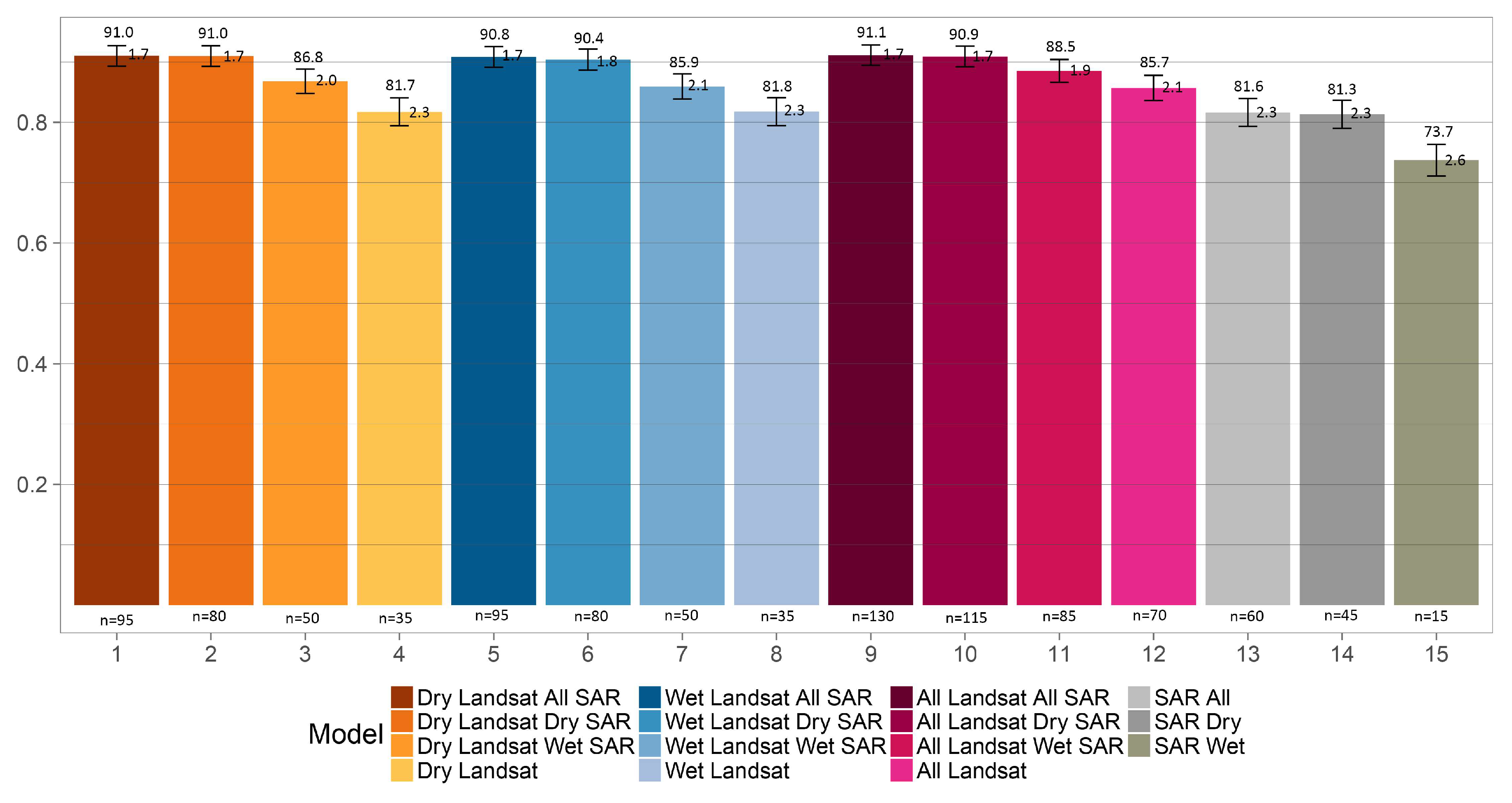
The model that scored the highest overall accuracy of 91.1 ± 1.7% was the one that incorporated Landsat and PALSAR metrics from both the dry and wet seasons (Model #9, Table 3, Figure 4). Its accuracy statistics are shown in Table 4, and the resulting map can be seen in Figure 5a. This model included 130 parameters and the ten most important ones, according to the mean decrease in the Gini index [63], can be seen in Figure S1.
Another five models (#1, 2, 5, 6, and 10) also scored very high overall accuracies (from 90.4 ± 1.8% to 91 ± 1.7%), i.e., within the confidence interval of the best-performing model. The six top performing models were able to map the main savannah types with similar per class accuracies (Figure 6; Table S2).
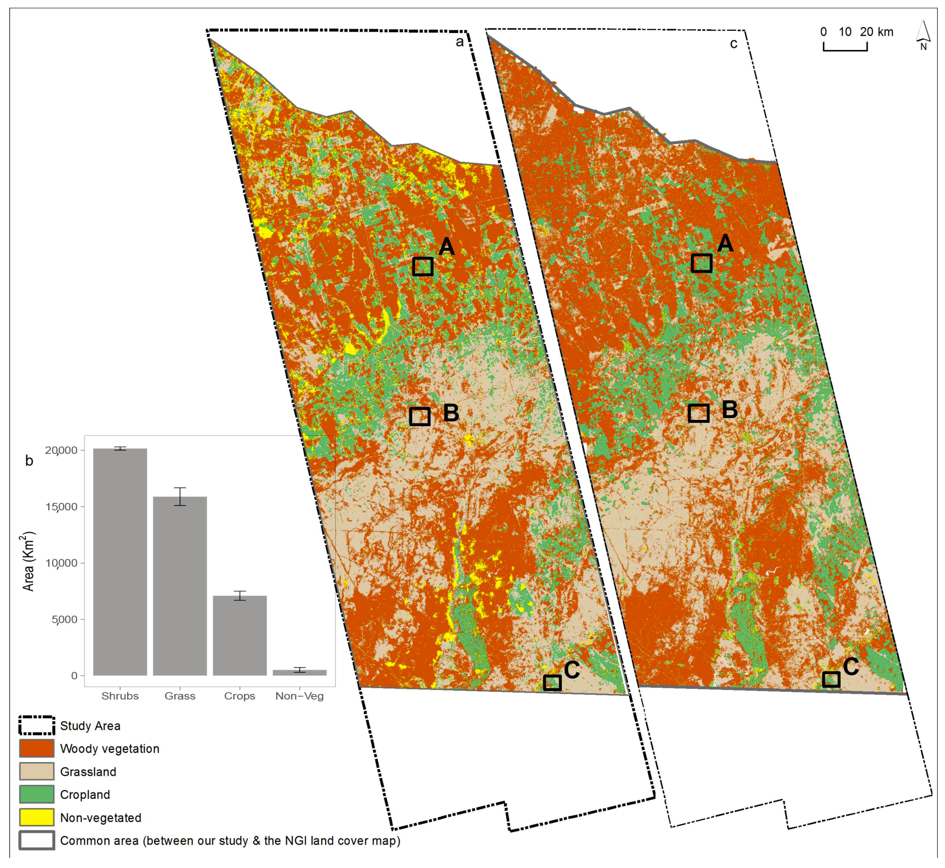
According to the “All Landsat All SAR” model (#9), woody vegetation and grassland were the most prevalent land cover classes, with 20,833 km2 (95% CI: 165 km2, i.e., 51 ± 0.4% of the study area) and 13,485 km2 (95% CI: 569 km2, i.e., 33 ± 1.5%), respectively. Cropland was the third largest (5930 ± 501 km2 or 15 ± 1.2% of the study area), while non-vegetated land occupied 3338 km2 (95% CI: 710 km2, i.e., 8 ± 1.7% of the study area).
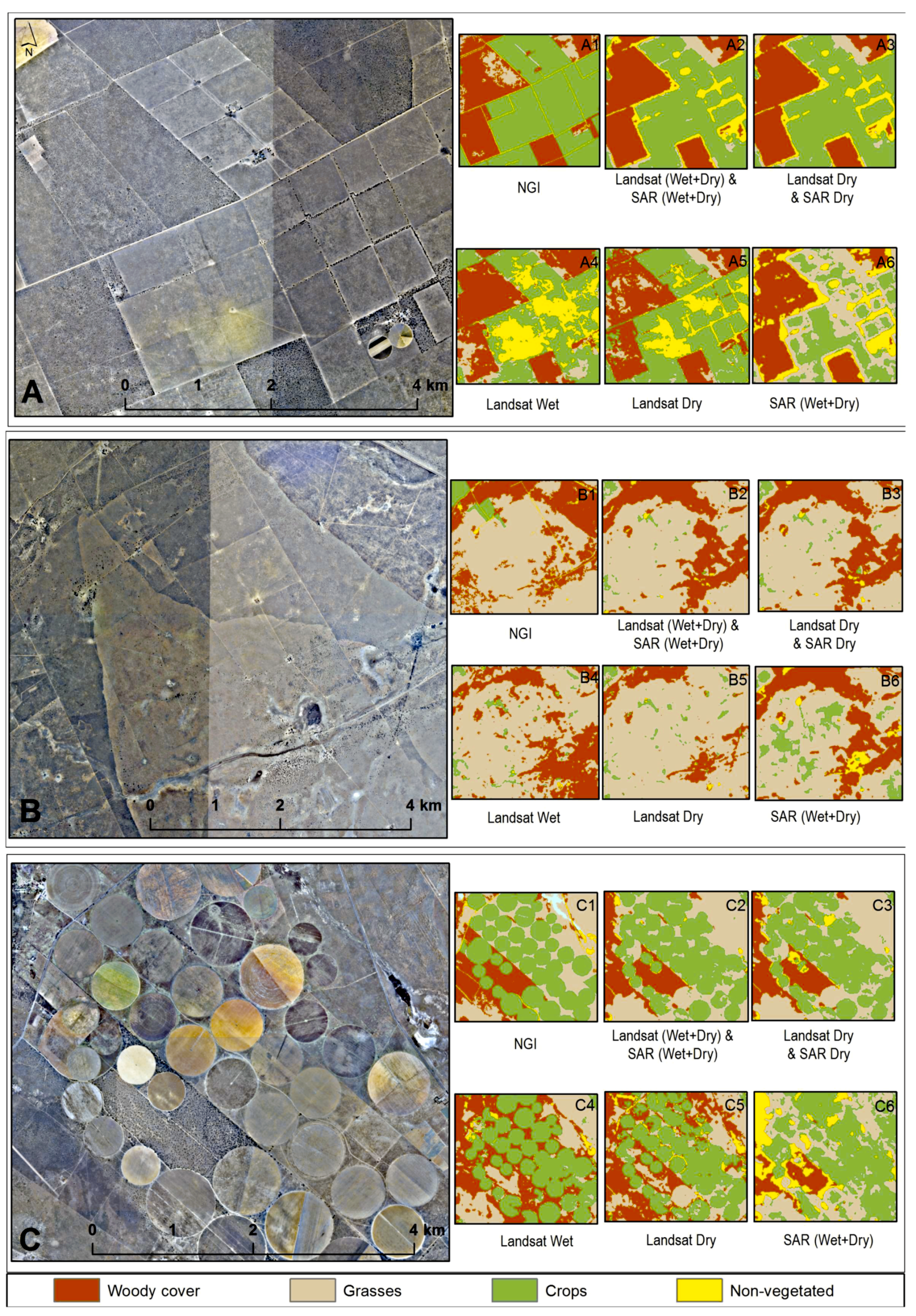
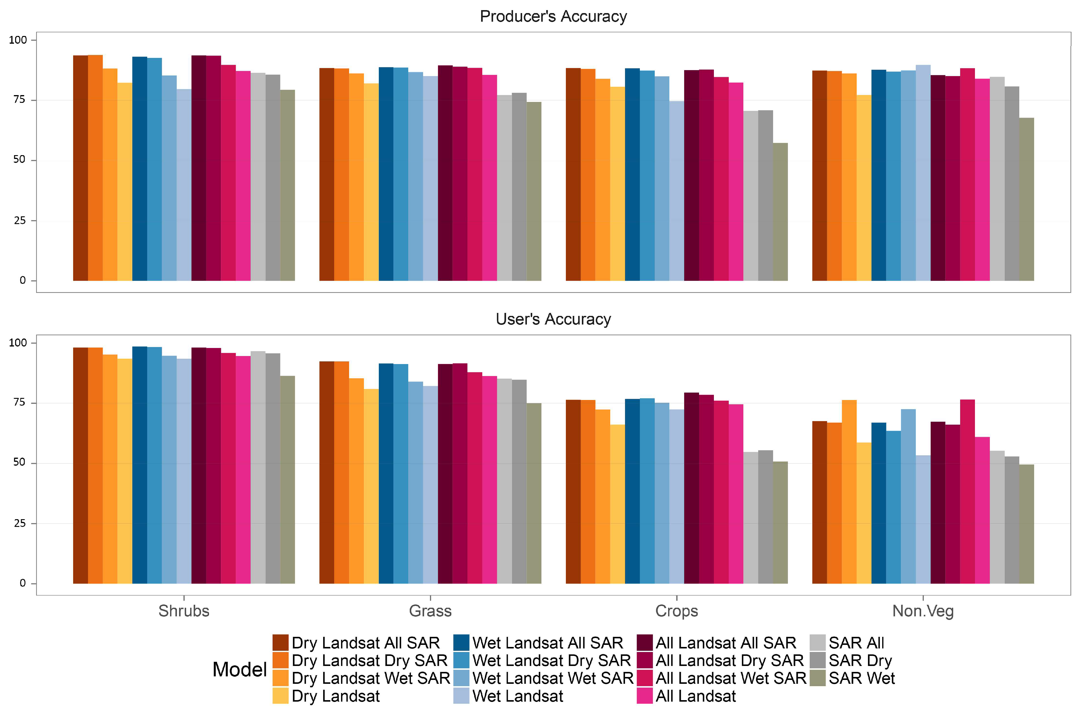
The most reliably mapped class was woody cover, with user’s and producer’s accuracies of 98.1% and 93.7%, respectively (Table 4). All classes demonstrated user’s and producer’s accuracies of over ~80%, with the exception of the user’s accuracy for the non-vegetated land (67.3%). The main source of error came from the commission of this land cover type, which can often occur when attempting to map classes that cover smaller areas [32,64]. Moreover, there is a degree of confusion between the grassland and cropland classes, which resulted in the relatively large confidence interval for cropland, even larger for grassland. This is also anticipated as a number of crops cultivated in the region (e.g., maize) have similar spectral properties to certain grasses [65]. In general, well-irrigated (pivot) fields were well mapped (Figure 7C), while smaller scale agriculture was less so (Figure 7A).
Our best performing model (Figure 5a) is spatially similar to the 10 × 10 m land cover map produced by the NGI for the Northwest Province in 2010 using SPOT 5 data (Figure 5c) [43]. We used the NGI map to compare our results in the absence of ground truth data, other than the very high-resolution aerial photography. The two maps follow similar general patterns with regards to the extent of woody cover, cropland and grassland. If the NGI data are considered as the reference, then our land cover map manifests a general underestimation of woody vegetation and cropland and a respective overestimation of grassland and non-vegetated land. We compared the NGI land cover with our best-performing model statistically: considering each land cover class separately, the data were first aggregated into percentage cover for 1 km grid cells. Pearson’s correlation tests were then applied to the corresponding pixels. This is considered a robust approach for comparing land cover as it minimises errors caused by geolocation and pixel misalignment [66]. The correlations were the highest for the cropland class (94.4%), followed by woody vegetation (74.5%) and grassland (61.7%), while a relatively low correlation was found for the non-vegetated class (54.5%).
Overall, the Landsat-only models were more accurate than the PALSAR models. The latter performed marginally worse than their optical counterparts, with overall accuracies of 81.6% (±2.3%) for the SAR model with both wet and dry season parameters (All SAR); 81.3% (±2.3%) for the dry season model (dry SAR) and 73.7% (±2.6%) for the wet season model (wet SAR), respectively (Figure 4). However, the PALSAR imagery were very effective in identifying woody cover, achieving very low commission errors: 3.4% for the “all SAR” and 4.2% for the “dry SAR”. The “wet SAR” model was not as successful, scoring a much higher woody vegetation commission error of 13.6% (Table S2). All other classes generally had higher commission and omission errors than the Landsat-based models, with the exception of the producer’s accuracy of the non-vegetated areas achieved by the “all SAR” and the “dry SAR” models (Table S2, Figure 6). Most interestingly, the results also show that the combination of the optical with the L-band SAR data improved the predictions, especially when the dry season PALSAR data were added to the models (Figure 4 and Figure 5; Table S2).
The most commonly employed approach of using dry season optical data did not prove to be more accurate than its wet season counterpart. The overall accuracies for both models were very similar, with the wet model actually performing slightly better: 81.8 ± 2.3% for the wet season and 81.7 ± 2.3% for the dry season, respectively (Figure 4). The wet season model also scored lower grassland and cropland commission errors, as well as lower grassland and non-vegetated omission errors, than did the dry season model (Figure 6, Table S2). Most importantly, when the wet season data were added to the ‘dry’ models, results always improved for all land cover types (Figure 6, Table S2).
Similarly, when SAR data were used in the model, the addition of the wet season data improved the model performance for most land cover types. With the exception of the producer’s accuracy for the grassland and the cropland and of the user’s accuracy for the latter, in all other cases the per-class accuracies increased when the wet season data were added.
4. Discussion
It is commonly understood that savannah landscapes are difficult to map, mostly due to the low inter-class but high intra-class spectral variability, confounded by seasonal and within-pixel variation [32,67]. Our best performing model, incorporating 130 parameters and estimated from dry and wet season optical and radar data, was able to achieve a high overall accuracy (91.1 ± 1.7%), as well as user’s and producer’s accuracies ranging from 80% to 98% for woody cover, grasses and crops. These three land cover types together occupy 92% of the study area in southern Africa. Difficulties were identified and high commission errors were produced when attempting to discriminate the non-vegetated areas (32.7%). This was anticipated and explained by both the low coverage of the area by such land cover types (8%), as well as the spectral confusion with the fallow land [32,64]. The latter was also noted by Eggen et al. [67] in their Landsat-based Ethiopian study, where they report very low accuracies for the barren class (54% user’s and 48% producer’s accuracy).
Our results, produced from multi-sensor and multi-season data, were similar to the accuracy achieved using coarser resolution data by Mishra et al. [68] who employed MODIS annual and intra-annual vegetation indices in a southern African savannah (Central Kalahari, Botswana). They presented overall accuracies of 93% when attempting to map the six main morphological vegetation types (woodland, dense shrub land, open shrub land, very open shrub land, grassland and pans/bare areas), which were very similar to ours (91.1%). The very high accuracy achieved with the MODIS data is commendable, especially since the methodology suggested by Mishra et al. [68] does not involve an onerous multi-sensor undertaking. However, when a finer resolution mapping product is required, MODIS-based approaches are not sufficient, and more complicated sensor fusion techniques need to be considered: for instance the one proposed in our study, or Landsat-MODIS fusions (e.g., STARFM [69] and ESTARFM [70]).
The use of metrics was also identified as being beneficial for land cover mapping by Müller et al. [32] in a study on another savannah environment in the Brazilian Cerrado, which was however much wetter. They used Landsat time series to map cropland, pasture and natural savannah vegetation and achieved a very similar overall accuracy (93%). They make a note that such high accuracies were possible due to the temporal depth of their study period, which was 3 years. In our study, we had to resort to using a slightly longer period (5 years) due to data availability and cloud contamination issues (Figure 3). The use of a 5-year compositing epoch may result in some land cover changes occurring within our study period. However, most change processes in savannahs (e.g., shrub encroachment, overgrazing, and overexploitation of woody shrubs and trees for fuelwood) are gradual transitions, which reduces the risk of abrupt conversions.
4.1. Landsat or PALSAR? or Both?
Radar data are known for their ability to map certain savannah vegetation properties, such as woody and canopy structure and volume [26,71]. Here we tested their fitness for mapping different savannah land cover types. When it came to the ability to identify woody cover, it was the combination of PALSAR dry and wet season metrics that produced the lowest commission errors (3.4%) and outperformed all other optical-only model combinations. This is in support of a number of studies who tested the performance of SAR data when mapping woody vegetation or the percentage of woody cover. Naidoo et al. [7] compared L-band PALSAR dry-season data with Random Forest models incorporating Landsat bands and vegetation and textural indices from different seasons, in order to map a woody canopy cover in an area within the Kruger National Park in South Africa. They found that the SAR-only models outperformed the best Landsat-only model by 9% (R2 = 0.81 and R2 = 0.72, respectively).
Our results, however, also showed that the Landsat-based models were generally slightly better than their SAR-based counterparts in identifying the other three targeted savannah land cover types. Walker et al. [72], in their study in the southeastern Brazilian Amazon, along with Laurin et al. [73], who compared SAR and optical classifications of 8 land cover classes in the West African region, have found that Landsat-based models performed better than PALSAR-based ones. In a more similar savannah environment in the Limpopo Province of South Africa, Higginbottom et al. [28] also tested the performance of models incorporating Landsat and PALSAR data. They mapped the fractional woody vegetation cover and used the global annual PALSAR mosaics, rather than the actual data we use here (http://www.eorc.jaxa.jp/ALOS/en/palsar_fnf/fnf_index.htm). They found that the Landsat-based models outperformed the PALSAR-based ones. However, the amount of Landsat imagery available, which makes the use of metrics more effective [32], renders the comparison with the relatively sparse PALSAR archive somewhat disproportionate: the SAR only models and the respective dry and wet season GLCM texture variables were developed from data gathered over one year only (2008; Table 2), while hundreds of Landsat images were involved in the calculations of the spectral-temporal variability metrics (Table 1). Still, the top five variables of the best-performing model, out of a total of 130, were all calculated from the PALSAR data (Figure S1), which is a clear indication of the importance of incorporating radar data in savannah land cover mapping efforts.
We found that multi-sensor combinations performed better than optical- or radar-only models: our dry season Landsat result (Figure 7(A5,B5,C5)) was improved by ~10% when the dry season SAR data were included in the model (Figure 7(A3,B3,C3)), bringing the overall accuracy up from ~81% to ~91%, almost the maximum achieved by any model combinations. This is in agreement with Naidoo et al. [7] who found that the combination of multi-sensor data produces the highest overall accuracies, reporting an improvement of 8% and 17% from the PALSAR-only and Landsat-only models, respectively. Laurin et al. [73] also compared PALSAR and optical (Landsat and AVNIR-2) land cover classifications in a wet tropical area and reported an improvement from the multi-sensor integration. In another study in the southeastern Brazilian Amazon, Walker et al. [72] compared PALSAR-based model results to Landsat ones and concluded that multi-sensor and multi-temporal radar and optical data is the way forward.
Given the promising results achieved by [26,74] with the RADARSAT-2 C-band when mapping savannah woody vegetation structure and by [75] who combined the Sentinel-1 C-band and Sentinel-2 data (with improved spatial, spectral and temporal resolutions compared to the Landsat data used in this study) in order to map land cover in a Mediterranean environment (overall accuracy =~94%, k = 0.928), it is anticipated that the synergy between the two Sentinels should provide considerable support in the efforts to accurately map savannah land cover.
4.2. Dry or Wet? or Both?
Using dry season optical data alone to map savannah land cover types, as in the case of most land cover mapping studies [76,77], produced a very similar overall accuracy (~82 ± 2%) and very similar omission and commission errors to their wet season counterparts. Wet season data, however, are inherently problematic due to the fact that cloud contamination and Landsat data availability is often limited in many dryland regions [78]. It is, therefore, reasonable that most analysts favour the use of dry season data since the accuracies achieved are relatively high, especially for mapping woody vegetation (with commission errors in our study of 6%). However, we also found that the combination of dry with wet season metrics improved results (an overall accuracy improvement of ~4% and per class statistics improvements throughout) and it is this approach that should be preferred if enough data are available. This is in agreement with Higginbottom et al. [28] who tested fractional woody cover estimation models with metrics estimated from the dry and the wet period and reported higher accuracies when data from both seasons were used. The higher temporal resolution of the Sentinel-2 data should therefore provide the means for improved savannah land cover mapping endeavours.
The PALSAR dry season model (Model #14 in Table 3) outperformed the wet season one (Model #15 in Table 3) in all mapped land cover classes (Table S2). It is also worth noting that the dry season HV backscatter outscored all other parameters as the best-performing model according to the mean variance Gini index (Figure S1). However, the wet season HV polarisation data were missing for our area and period of study and, therefore, we are unable to directly compare the dry and wet season SAR model performances. Nevertheless, we did find that the addition of the wet season SAR data to their dry season counterparts increased the model performance (Figure 4 and Figure 5; Table S2); consequently, if radar data from both seasons are available (e.g., Sentinel-1 C-band), this should be the preferred methodological approach for savannah land cover mapping.
An approach that has not been considered here but could potentially improve results is not to consider dry and wet season predictors separately, but to combine them. For example, a difference between a mean wet and a mean dry vegetation index could be calculated for the optical data and a similar mean index estimated from the different seasons and polarisations of the SAR data. On a similar note, another approach could be to use a phenological analysis to derive surrogate maps of the vegetated land cover types by analyzing the temporal evolution of an index (e.g., NDVI; [79]). High temporal-resolution data are required for this and, as a consequence of this, coarser resolution data, such as MODIS, have traditionally been employed [80]. However, new approaches that extract phenology estimates using high-resolution imagery from a single season [81], or that combine high spatial-resolution data (e.g., GF-1) with phenological parameters from high temporal-resolution sensors (e.g., MODIS) to classify land cover, have recently been developed [82]. To this end, our ability to now employ Sentinel-2 data, with their high repeat frequency, offers a promising outlook.
5. Conclusions
Savannah ecosystems cover a fifth of the Earth’s surface and are one of the least studied and most difficult biomes to map, increasingly undergoing processes of degradation. The most recent attempts to map the savannah land cover have incorporated optical or radar EO data from the dry season or from different phenological periods. In this study, we focus on a southern African area to assess how accurately woody vegetation, grassland, cropland and non-vegetated areas can be mapped in order to provide assistance in future attempts to characterise and monitor savannah land cover. Given the overall accuracy and the per class statistics produced from the 15 models tested, as well as the spatial similarity of an independent finer-scale land cover map with our results, it is safe to conclude that the main cover types of woody vegetation, grassland and crops can be accurately mapped, when optical and radar data from the dry and wet seasons are integrated. The recent developments in EO sensors and the open-access availability of higher spectral, spatial and temporal resolution data (e.g., the European Space Agency’s Sentinel-1 and Sentinel-2 satellites), offer promising pathways for accurate multi-sensor and multi-season savannah land cover mapping.
Supplementary Materials
The following are available online at https://www.mdpi.com/2072-4292/10/4/499/s1, Table S1: Availability of cloud-free observations per pixel per 5-year seasonal window. Table S2: Per-class accuracy statistics for the 15 models tested; Figure S1: Ten most important variables for the “All Landsat All SAR” Random Forest model (model #9 in Figure 4) according to the Mean Decrease Gini index [61]. fbd_hv: dry season HV PALSAR backscatter; fbd_hv_variance: the Grey-Level Co-occurrence Matrix (GLCM) variance layer for the dry season HV backscatter; fbd_hv_mean: the Grey-Level Co-occurrence Matrix (GLCM) mean layer for the dry season HV backscatter; _9: the 9 × 9 window GLCM statistics calculations; _3: the 3 × 3 window GLCM statistics calculations; B1, B2, …: Landsat bands; p25, p50: 25th, 50th percentiles
Acknowledgments
This work forms part of the LanDDApp EU FP7 Marie Curie Career Integration project (PCIG12-GA-2012-3374327). Thomas Higginbottom is funded by a Manchester Metropolitan University (MMU) Research Fellowship. We are grateful to the USGS, JAXA, and the NGI for providing the data used in this study. The authors declare no personal or financial conflicts of interest.
Author Contributions
The paper was conceived and designed by Elias Symeonakis. Thomas Higginbottom analysed the imagery with technical support from Andreas Mueller and Kyriaki Petroulaki. The manuscript was written by Elias Symeonakis with input from Thomas Higginbottom.
Conflicts of Interest
The authors declare no conflict of interest.
References
- Scholes, R.J.; Walker, B.H. An African Savanna: Synthesis of the Nylsvley Study; Cambridge University Press: Cambridge, UK, 1993. [Google Scholar]
- Wessels, K.; Prince, S.; Malherbe, J.; Small, J.; Frost, P.; Van Zyl, D. Can human-induced land degradation be distinguished from the effects of rainfall variability? A case study in South Africa. J. Arid Environ. 2007, 68, 271–297. [Google Scholar] [CrossRef]
- Wessels, K.J.; van den Bergh, F.; Scholes, R.J. Limits to detectability of land degradation by trend analysis of vegetation index data. Remote Sens. Environ. 2012, 125, 10–22. [Google Scholar] [CrossRef]
- Poulter, B.; Frank, D.; Ciais, P.; Myneni, R.B.; Andela, N.; Bi, J.; Broquet, G.; Canadell, J.G.; Chevallier, F.; Liu, Y.Y. Contribution of semi-arid ecosystems to interannual variability of the global carbon cycle. Nature 2014, 509, 600–603. [Google Scholar] [CrossRef] [PubMed]
- Sankaran, M.; Ratnam, J.; Hanan, N. Woody cover in African savannas: The role of resources, fire and herbivory. Glob. Ecol. Biogeogr. 2008, 17, 236–245. [Google Scholar] [CrossRef]
- Sankaran, M.; Hanan, N.P.; Scholes, R.J.; Ratnam, J.; Augustine, D.J.; Cade, B.S.; Gignoux, J.; Higgins, S.I.; Le Roux, X.; Ludwig, F.; et al. Determinants of woody cover in African savannas. Nature 2005, 438, 846. [Google Scholar] [CrossRef] [PubMed]
- Naidoo, L.; Mathieu, R.; Main, R.; Wessels, K.; Asner, G.P. L-band Synthetic Aperture Radar imagery performs better than optical datasets at retrieving woody fractional cover in deciduous, dry savannahs. Int. J. Appl. Earth Obs. Geoinform. 2016, 52, 54–64. [Google Scholar] [CrossRef]
- Schneibel, A.; Frantz, D.; Röder, A.; Stellmes, M.; Fischer, K.; Hill, J. Using Annual Landsat Time Series for the Detection of Dry Forest Degradation Processes in South-Central Angola. Remote Sens. 2017, 9, 905. [Google Scholar] [CrossRef]
- UNCCD. Global Land Outlook; UNCCD: Paris, France, 2017; p. 338. [Google Scholar]
- Symeonakis, E.; Higginbottom, T. Bush Encroachment Monitoring Using Multi-Temporal Landsat Data and Random Forests. Int. Arch Photogramm. Remote Sens. Spat. Inf. Sci. 2014, 40, 29–35. [Google Scholar] [CrossRef]
- Maestre, F.T.; Eldridge, D.J.; Soliveres, S.; Kéfi, S.; Delgado-Baquerizo, M.; Bowker, M.A.; García-Palacios, P.; Gaitán, J.; Gallardo, A.; Lázaro, R. Structure and functioning of dryland ecosystems in a changing world. Annu. Rev. Ecol. Evolut. Syst. 2016, 47, 215–237. [Google Scholar] [CrossRef] [PubMed]
- Millennium Ecosystem Assessment. Ecosystems and human well-being: Synthesis; World Resources Institute: Washington, DC, USA, 2005. [Google Scholar]
- Kuemmerle, T.; Erb, K.; Meyfroidt, P.; Müller, D.; Verburg, P.H.; Estel, S.; Haberl, H.; Hostert, P.; Jepsen, M.R.; Kastner, T.; et al. Challenges and opportunities in mapping land use intensity globally. Curr. Opin. Environ. Sustain. 2013, 5, 484–493. [Google Scholar] [CrossRef] [PubMed]
- Lehmann, E.A.; Wallace, J.F.; Caccetta, P.A.; Furby, S.L.; Zdunic, K. Forest cover trends from time series Landsat data for the Australian continent. Int. J. Appl. Earth Obs. Geoinform. 2013, 21, 453–462. [Google Scholar] [CrossRef]
- Wulder, M.A.; Masek, J.G.; Cohen, W.B.; Loveland, T.R.; Woodcock, C.E. Opening the archive: How free data has enabled the science and monitoring promise of Landsat. Remote Sens. Environ. 2012, 122, 2–10. [Google Scholar] [CrossRef]
- Bastin, J.-F.; Berrahmouni, N.; Grainger, A.; Maniatis, D.; Mollicone, D.; Moore, R.; Patriarca, C.; Picard, N.; Sparrow, B.; Abraham, E.M.; et al. The extent of forest in dryland biomes. Science 2017, 356, 635–638. [Google Scholar] [CrossRef] [PubMed]
- Kennedy, R.E.; Andréfouët, S.; Cohen, W.B.; Gómez, C.; Griffiths, P.; Hais, M.; Healey, S.P.; Helmer, E.H.; Hostert, P.; Lyons, M.B. Bringing an ecological view of change to Landsat-based remote sensing. Front. Ecol. Environ. 2014, 12, 339–346. [Google Scholar] [CrossRef] [Green Version]
- Senf, C.; Leitão, P.J.; Pflugmacher, D.; van der Linden, S.; Hostert, P. Mapping land cover in complex Mediterranean landscapes using Landsat: Improved classification accuracies from integrating multi-seasonal and synthetic imagery. Remote Sens. Environ. 2015, 156, 527–536. [Google Scholar] [CrossRef]
- Knorn, J.; Rabe, A.; Radeloff, V.C.; Kuemmerle, T.; Kozak, J.; Hostert, P. Land cover mapping of large areas using chain classification of neighboring Landsat satellite images. Remote Sens. Environ. 2009, 113, 957–964. [Google Scholar] [CrossRef]
- Hansen, M.C.; Egorov, A.; Roy, D.P.; Potapov, P.; Ju, J.; Turubanova, S.; Kommareddy, I.; Loveland, T.R. Continuous fields of land cover for the conterminous United States using Landsat data: First results from the Web-Enabled Landsat Data (WELD) project. Remote Sens. Lett. 2011, 2, 279–288. [Google Scholar] [CrossRef]
- Gong, P.; Wang, J.; Yu, L.; Zhao, Y.; Zhao, Y.; Liang, L.; Niu, Z.; Huang, X.; Fu, H.; Liu, S.; et al. Finer resolution observation and monitoring of global land cover: First mapping results with Landsat TM and ETM+ data. Int. J. Remote Sens. 2013, 34, 2607–2654. [Google Scholar] [CrossRef]
- de la Cruz, M.; Quintana-Ascencio, P.F.; Cayuela, L.; Espinosa, C.I.; Escudero, A. Comment on “The extent of forest in dryland biomes”. Science 2017, 358. [Google Scholar] [CrossRef] [PubMed]
- Griffith, D.M.; Lehmann, C.E.R.; Strömberg, C.A.E.; Parr, C.L.; Pennington, R.T.; Sankaran, M.; Ratnam, J.; Still, C.J.; Powell, R.L.; Hanan, N.P.; et al. Comment on “The extent of forest in dryland biomes”. Science 2017, 358. [Google Scholar] [CrossRef] [PubMed]
- Schepaschenko, D.; Fritz, S.; See, L.; Laso Bayas, J.C.; Lesiv, M.; Kraxner, F.; Obersteiner, M. Comment on “The extent of forest in dryland biomes”. Science 2017, 358. [Google Scholar] [CrossRef] [PubMed]
- Olsson, A.D.; van Leeuwen, W.J.D.; Marsh, S.E. Feasibility of Invasive Grass Detection in a Desertscrub Community Using Hyperspectral Field Measurements and Landsat TM Imagery. Remote Sens. 2011, 3, 2283. [Google Scholar] [CrossRef]
- Mathieu, R.; Naidoo, L.; Cho, M.A.; Leblon, B.; Main, R.; Wessels, K.; Asner, G.P.; Buckley, J.; Van Aardt, J.; Erasmus, B.F.N.; et al. Toward structural assessment of semi-arid African savannahs and woodlands: The potential of multitemporal polarimetric RADARSAT-2 fine beam images. Remote Sens. Environ. 2013, 138, 215–231. [Google Scholar] [CrossRef]
- Shimada, M.; Itoh, T.; Motooka, T.; Watanabe, M.; Shiraishi, T.; Thapa, R.; Lucas, R. New global forest/non-forest maps from ALOS PALSAR data (2007–2010). Remote Sens. Environ. 2014, 155, 13–31. [Google Scholar] [CrossRef]
- Higginbottom, T.; Symeonakis, E.; Meyer, H.; van der Linden, S. Mapping Woody Cover in Semi-arid Savannahs using Multi-seasonal Composites from Landsat Data. ISPRS J. Photogramm. Remote Sens. 2017; in press. [Google Scholar]
- Kanniah, K.D.; Beringer, J. Tropical Savanna Ecosystems. Int. Encycl. Geogr. 2017. [Google Scholar] [CrossRef]
- Hüttich, C.; Gessner, U.; Herold, M.; Strohbach, B.J.; Schmidt, M.; Keil, M.; Dech, S. On the suitability of MODIS time series metrics to map vegetation types in dry savanna ecosystems: A case study in the Kalahari of NE Namibia. Remote Sens. 2009, 1, 620–643. [Google Scholar] [CrossRef]
- Hüttich, C.; Herold, M.; Wegmann, M.; Cord, A.; Strohbach, B.; Schmullius, C.; Dech, S. Assessing effects of temporal compositing and varying observation periods for large-area land-cover mapping in semi-arid ecosystems: Implications for global monitoring. Remote Sens. Environ. 2011, 115, 2445–2459. [Google Scholar] [CrossRef]
- Müller, H.; Rufin, P.; Griffiths, P.; Barros Siqueira, A.J.; Hostert, P. Mining dense Landsat time series for separating cropland and pasture in a heterogeneous Brazilian savanna landscape. Remote Sens. Environ. 2015, 156, 490–499. [Google Scholar] [CrossRef]
- Schuster, C.; Schmidt, T.; Conrad, C.; Kleinschmit, B.; Förster, M. Grassland habitat mapping by intra-annual time series analysis—Comparison of RapidEye and TerraSAR-X satellite data. Int. J. Appl. Earth Obs. Geoinform. 2015, 34, 25–34. [Google Scholar] [CrossRef]
- Bleyhl, B.; Baumann, M.; Griffiths, P.; Heidelberg, A.; Manvelyan, K.; Radeloff, V.C.; Zazanashvili, N.; Kuemmerle, T. Assessing landscape connectivity for large mammals in the Caucasus using Landsat 8 seasonal image composites. Remote Sens. Environ. 2017, 193, 193–203. [Google Scholar] [CrossRef]
- Schwieder, M.; Leitão, P.J.; da Cunha Bustamante, M.M.; Ferreira, L.G.; Rabe, A.; Hostert, P. Mapping Brazilian savanna vegetation gradients with Landsat time series. Int. J. Appl. Earth Obs. Geoinform. 2016, 52, 361–370. [Google Scholar] [CrossRef]
- Thomas, D.S.G.; Twyman, C.; Osbahr, H.; Hewitson, B. Adaptation to climate change and variability: Farmer responses to intra-seasonal precipitation trends in South Africa. Clim. Chang. 2007, 83, 301–322. [Google Scholar] [CrossRef]
- SANBI. The Vegetation Map of South Africa, Lesotho and Swaziland; Mucina, L., Rutherford, M.C., Powrie, L.W., Eds.; SANBI: Pretoria, South Africa, 2012. [Google Scholar]
- Arp, R.; Fraser, G.; Hill, M. Quantifying the economic water savings benefit of water hyacinth (Eichhornia crassipes) control in the Vaalharts Irrigation Scheme. Water SA 2017, 43, 58–66. [Google Scholar] [CrossRef]
- DAFF. Abstract of Agricultural Statistics; DAFF: Canberra, Australia, 2017.
- Agribook. The Agri Handbook for South Africa, 6th ed.; RainbowSA: Kerala, India, 2017; p. 464. [Google Scholar]
- Di Gregorio, A.; Jansen, L. Land Cover Classification Systems–Classification Concepts and User Manual for Software Version 1.0; FAO Environment and Natural Resources Service Series; Food and Agriculture Organization: Rome, Italy, 2005. [Google Scholar]
- NGI. The National Geospatial Information (NGI) Colour Digital Aerial Imagery at 0.5m GSD (2008–2016); NGI: Manchester, UK, 2017. [Google Scholar]
- Verhulp, J.; Denner, M. The Development of the South African National Land Cover Mapping Program: Progress and Challenges. 2010. Available online: http://www.africageoproceedings.org.za/wp-content/uploads/2014/08/119_Verhulp_Denner1.pdf (accessed on 19 March 2018).
- NGI. National Aerial Imagery of South Africa. In National Geo-Spatial Information; NGI: Manchester, UK, 2014; Available online: https://www.arcgis.com/home/item.html?id=9d01fa9041264cb283c353a5a613c81e (accessed on 19 March 2018).
- Masek, J.G.; Vermote, E.F.; Saleous, N.E.; Wolfe, R.; Hall, F.G.; Huemmrich, K.F.; Gao, F.; Kutler, J.; Lim, T.-K. A Landsat surface reflectance dataset for North America, 1990–2000. IEEE Geosci. Remote Sens. Lett. 2006, 3, 68–72. [Google Scholar] [CrossRef]
- Zhu, Z.; Woodcock, C.E. Object-based cloud and cloud shadow detection in Landsat imagery. Remote Sens. Environ. 2012, 118, 83–94. [Google Scholar] [CrossRef]
- Tucker, C.J. Red and photographic infrared linear combinations for monitoring vegetation. Remote Sens. Environ. 1979, 8, 127–150. [Google Scholar] [CrossRef]
- Hansen, M.; Potapov, P.; Moore, R.; Hancher, M.; Turubanova, S.; Tyukavina, A.; Thau, D.; Stehman, S.; Goetz, S.; Loveland, T. High-Resolution Global Maps of 21st-Century Forest Cover Change. Science 2013, 342, 850–853. [Google Scholar] [CrossRef] [PubMed]
- Maidment, R.I.; Grimes, D.; Black, E.; Tarnavsky, E.; Young, M.; Greatrex, H.; Allan, R.P.; Stein, T.; Nkonde, E.; Senkunda, S.; et al. A new, long-term daily satellite-based rainfall dataset for operational monitoring in Africa. Sci. Data 2017, 4, 170063. [Google Scholar] [CrossRef] [PubMed]
- Lee, J.-S.; Jurkevich, L.; Dewaele, P.; Wambacq, P.; Oosterlinck, A. Speckle filtering of synthetic aperture radar images: A review. Remote Sens. Rev. 1994, 8, 313–340. [Google Scholar] [CrossRef]
- Erdas Imagine 2013; Intergraph Geospatial: Huntsville, AL, USA, 2013.
- Miettinen, J.; Liew, S.C. Separability of insular Southeast Asian woody plantation species in the 50 m resolution ALOS PALSAR mosaic product. Remote Sens. Lett. 2011, 2, 299–307. [Google Scholar] [CrossRef]
- Wu, F.; Wang, C.; Zhang, H.; Zhang, B.; Tang, Y. Rice Crop Monitoring in South China With RADARSAT-2 Quad-Polarization SAR Data. IEEE Geosci. Remote Sens. Lett. 2011, 8, 196–200. [Google Scholar] [CrossRef]
- Dong, J.; Xiao, X.; Sheldon, S.; Biradar, C.; Duong, N.D.; Hazarika, M. A comparison of forest cover maps in Mainland Southeast Asia from multiple sources: PALSAR, MERIS, MODIS and FRA. Remote Sens. Environ. 2012, 127, 60–73. [Google Scholar] [CrossRef]
- Haralick, R.M. Statistical and structural approaches to texture. Proc. IEEE 1979, 67, 786–804. [Google Scholar] [CrossRef]
- Thapa, R.B.; Watanabe, M.; Motohka, T.; Shimada, M. Potential of high-resolution ALOS–PALSAR mosaic texture for aboveground forest carbon tracking in tropical region. Remote Sens. Environ. 2015, 160, 122–133. [Google Scholar] [CrossRef]
- Breiman, L. Random forests. Mach. Learn. 2001, 45, 5–32. [Google Scholar] [CrossRef]
- Pal, M. Random forest classifier for remote sensing classification. Int. J. Remote Sens. 2005, 26, 217–222. [Google Scholar] [CrossRef]
- R Development Core Team. R: A Language and Environment for Statistical Computing; R Foundation for Statistical Computing: Vienna, Austria, 2017. [Google Scholar]
- Olofsson, P.; Foody, G.M.; Stehman, S.V.; Woodcock, C.E. Making better use of accuracy data in land change studies: Estimating accuracy and area and quantifying uncertainty using stratified estimation. Remote Sens. Environ. 2013, 129, 122–131. [Google Scholar] [CrossRef]
- Cochran, W.G. Sample Techniques; John Wills & Sons: New York, NY, USA, 1977. [Google Scholar]
- Congalton, R.G.; Green, K. Assessing the Accuracy of Remotely Sensed Data: Principles and Practices; CRC Press: Boca Raton, USA, 2009. [Google Scholar]
- Owen, H.J.F.; Duncan, C.; Pettorelli, N. Testing the water: Detecting artificial water points using freely available satellite data and open source software. Remote Sens. Ecol. Conserv. 2015, 1, 61–72. [Google Scholar] [CrossRef]
- Olofsson, P.; Foody, G.M.; Herold, M.; Stehman, S.V.; Woodcock, C.E.; Wulder, M.A. Good practices for estimating area and assessing accuracy of land change. Remote Sens. Environ. 2014, 148, 42–57. [Google Scholar] [CrossRef]
- Tang, K.; Zhu, W.; Zhan, P.; Ding, S. An Identification Method for Spring Maize in Northeast China Based on Spectral and Phenological Features. Remote Sens. 2018, 10, 193. [Google Scholar] [CrossRef]
- Carreiras, J.M.B.; Jones, J.; Lucas, R.M.; Gabriel, C. Land use and land cover change dynamics across the Brazilian Amazon: Insights from extensive time-series analysis of remote sensing data. PLoS ONE 2014, 9, e104144. [Google Scholar] [CrossRef] [PubMed]
- Eggen, M.; Ozdogan, M.; Zaitchik, B.; Simane, B. Land Cover Classification in Complex and Fragmented Agricultural Landscapes of the Ethiopian Highlands. Remote Sens. 2016, 8, 1020. [Google Scholar] [CrossRef]
- Mishra, N.B.; Crews, K.A.; Miller, J.A.; Meyer, T. Mapping vegetation morphology types in southern Africa savanna using MODIS time-series metrics: A case study of central Kalahari, Botswana. Land 2015, 4, 197–215. [Google Scholar] [CrossRef]
- Gao, F.; Masek, J.; Schwaller, M.; Hall, F. On the blending of the Landsat and MODIS surface reflectance: Predicting daily Landsat surface reflectance. IEEE Trans. Geosci. Remote Sens. 2006, 44, 2207–2218. [Google Scholar]
- Knauer, K.; Gessner, U.; Fensholt, R.; Kuenzer, C. An ESTARFM Fusion Framework for the Generation of Large-Scale Time Series in Cloud-Prone and Heterogeneous Landscapes. Remote Sens. 2016, 8, 425. [Google Scholar] [CrossRef]
- Myburgh, H.C.; Olivier, J.C.; Mathieu, R.; Wessels, K.; Leblon, B.; Asner, G.; Buckley, J. SAR-to-LiDAR mapping for tree volume prediction in the Kruger National Park. In Proceedings of the IEEE International Geoscience and Remote Sensing Symposium (IGARSS), Vancouver, BC, Canada, 24–29 July 2011; pp. 1934–1937. [Google Scholar]
- Walker, W.S.; Stickler, C.M.; Kellndorfer, J.M.; Kirsch, K.M.; Nepstad, D.C. Large-Area Classification and Mapping of Forest and Land Cover in the Brazilian Amazon: A Comparative Analysis of ALOS/PALSAR and Landsat Data Sources. IEEE J. Sel. Top. Appl. Earth Obs. Remote Sens. 2010, 3, 594–604. [Google Scholar] [CrossRef]
- Laurin, G.V.; Liesenberg, V.; Chen, Q.; Guerriero, L.; Del Frate, F.; Bartolini, A.; Coomes, D.; Wilebore, B.; Lindsell, J.; Valentini, R. Optical and SAR sensor synergies for forest and land cover mapping in a tropical site in West Africa. Int. J. Appl Earth Obs. Geoinform. 2013, 21, 7–16. [Google Scholar] [CrossRef]
- Main, R.; Mathieu, R.; Kleynhans, W.; Wessels, K.; Naidoo, L.; Asner, G. Hyper-Temporal C-Band SAR for Baseline Woody Structural Assessments in Deciduous Savannas. Remote Sens. 2016, 8, 661. [Google Scholar] [CrossRef]
- Chatziantoniou, A.; Petropoulos, G.P.; Psomiadis, E. Co-Orbital Sentinel 1 and 2 for LULC mapping with emphasis on wetlands in a mediterranean setting based on machine learning. Remote Sens. 2017, 9, 1259. [Google Scholar] [CrossRef]
- Yang, J.; Prince, S.D. Remote sensing of savanna vegetation changes in Eastern Zambia 1972–1989. Int. J. Remote Sens. 2000, 21, 301–322. [Google Scholar] [CrossRef]
- Marston, C.; Aplin, P.; Wilkinson, D.; Field, R.; O’Regan, H. Scrubbing Up: Multi-Scale Investigation of Woody Encroachment in a Southern African Savannah. Remote Sens. 2017, 9, 419. [Google Scholar] [CrossRef]
- Wulder, M.A.; White, J.C.; Loveland, T.R.; Woodcock, C.E.; Belward, A.S.; Cohen, W.B.; Fosnight, E.A.; Shaw, J.; Masek, J.G.; Roy, D.P. The global Landsat archive: Status, consolidation, and direction. Remote Sens. Environ. 2016, 185, 271–283. [Google Scholar] [CrossRef]
- De Beurs, K.M.; Henebry, G.M. Spatio-temporal statistical methods for modelling land surface phenology. In Phenological Research: Methods for Environmental and Climate Change Analysis; Springer: Berlin, Germany, 2010; pp. 177–208. [Google Scholar]
- Jin, Y.; Sung, S.; Lee, D.; Biging, G.; Jeong, S. Mapping Deforestation in North Korea Using Phenology-Based Multi-Index and Random Forest. Remote Sens. 2016, 8, 997. [Google Scholar] [CrossRef]
- Vrieling, A.; Skidmore, A.K.; Wang, T.; Meroni, M.; Ens, B.J.; Oosterbeek, K.; O’Connor, B.; Darvishzadeh, R.; Heurich, M.; Shepherd, A.; et al. Spatially detailed retrievals of spring phenology from single-season high-resolution image time series. Int. J. Appl. Earth Obs. Geoinform. 2017, 59, 19–30. [Google Scholar] [CrossRef]
- Kong, F.; Li, X.; Wang, H.; Xie, D.; Li, X.; Bai, Y. Land Cover Classification Based on Fused Data from GF-1 and MODIS NDVI Time Series. Remote Sens. 2016, 8, 741. [Google Scholar] [CrossRef]
Figure 1.
The location of the study area in: (a) Africa, and (b) southern Africa. (c) The elevation within the study area.
Figure 1.
The location of the study area in: (a) Africa, and (b) southern Africa. (c) The elevation within the study area.
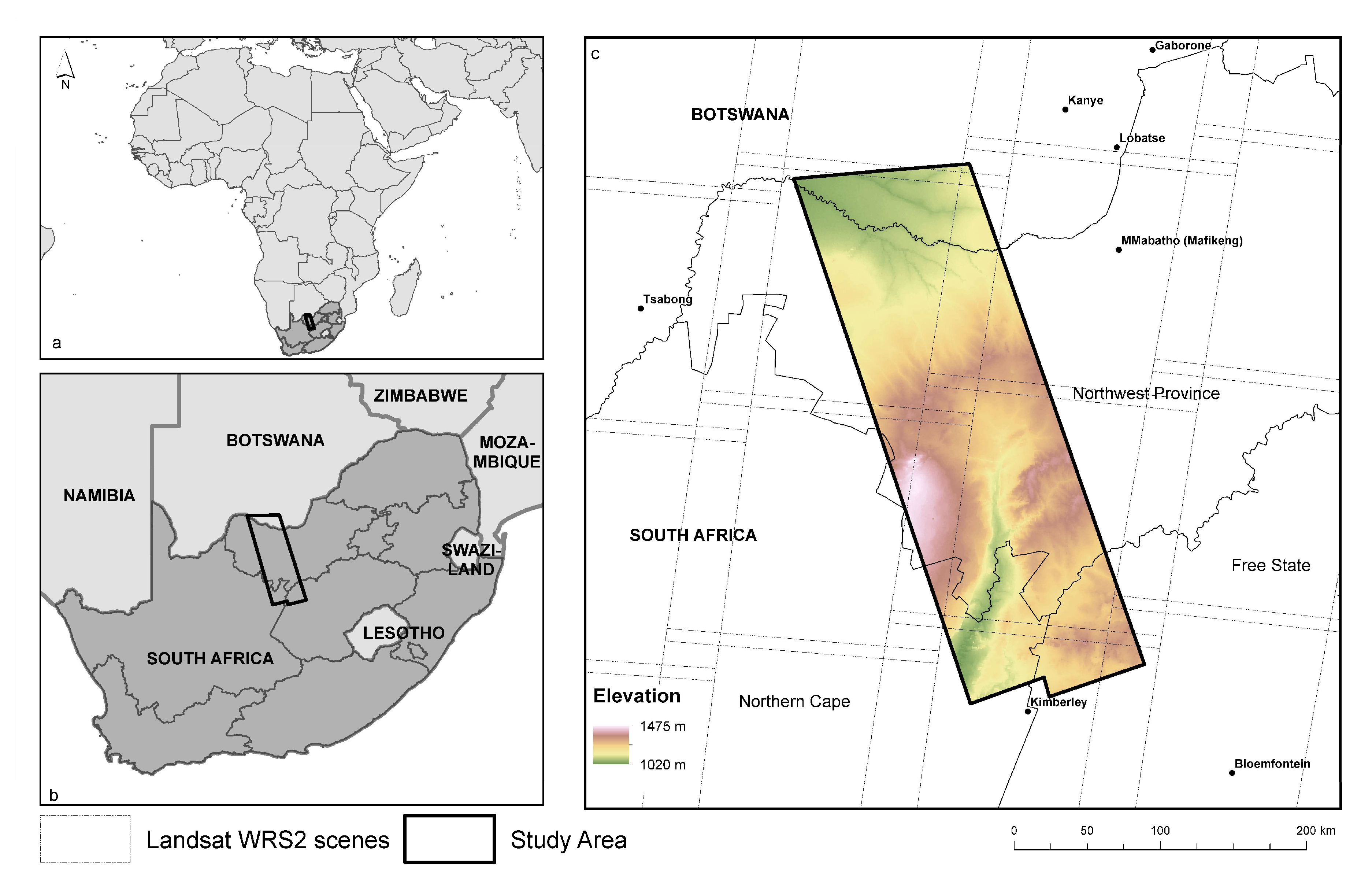
Figure 2.
Examples of the four main land cover classes of the study area: (a) woody vegetation; (b) grassland; (c) cropland, and (d) non-vegetated land.
Figure 2.
Examples of the four main land cover classes of the study area: (a) woody vegetation; (b) grassland; (c) cropland, and (d) non-vegetated land.
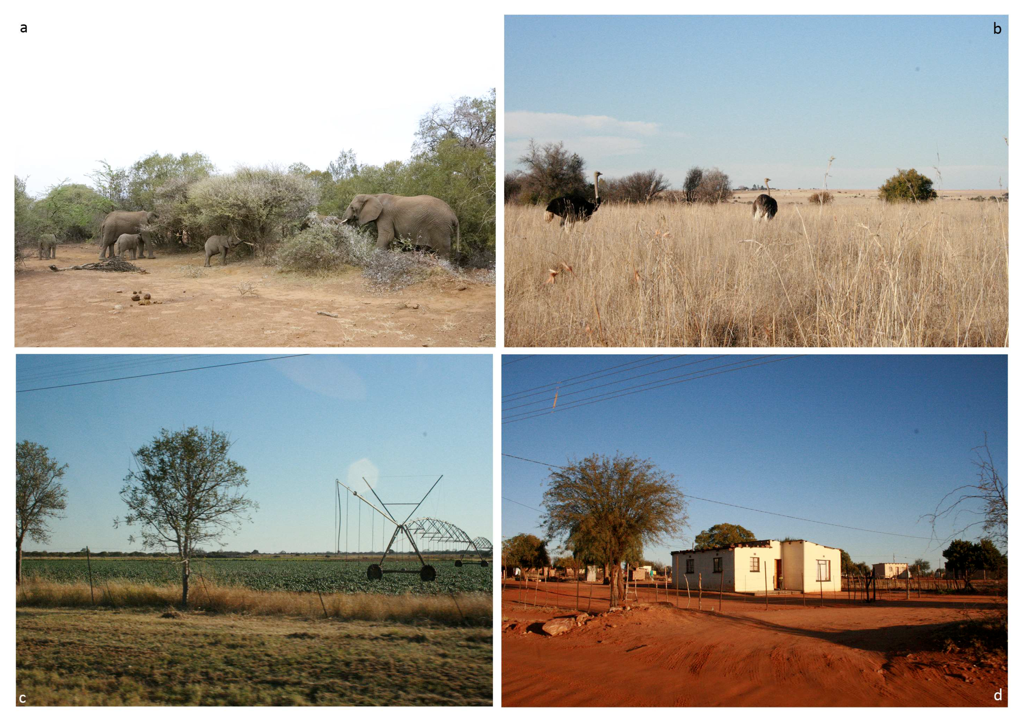
Figure 3.
Number of Landsat Thematic Mapper (TM) and Enhanced Thematic Mapper + (ETM+) observations over the study area for: (a) the dry seasons of the years 2007–2011 (2 June–1 October); (b) the respective wet seasons (21 November–31 March), and (c) the dry season of the year 2008.
Figure 3.
Number of Landsat Thematic Mapper (TM) and Enhanced Thematic Mapper + (ETM+) observations over the study area for: (a) the dry seasons of the years 2007–2011 (2 June–1 October); (b) the respective wet seasons (21 November–31 March), and (c) the dry season of the year 2008.
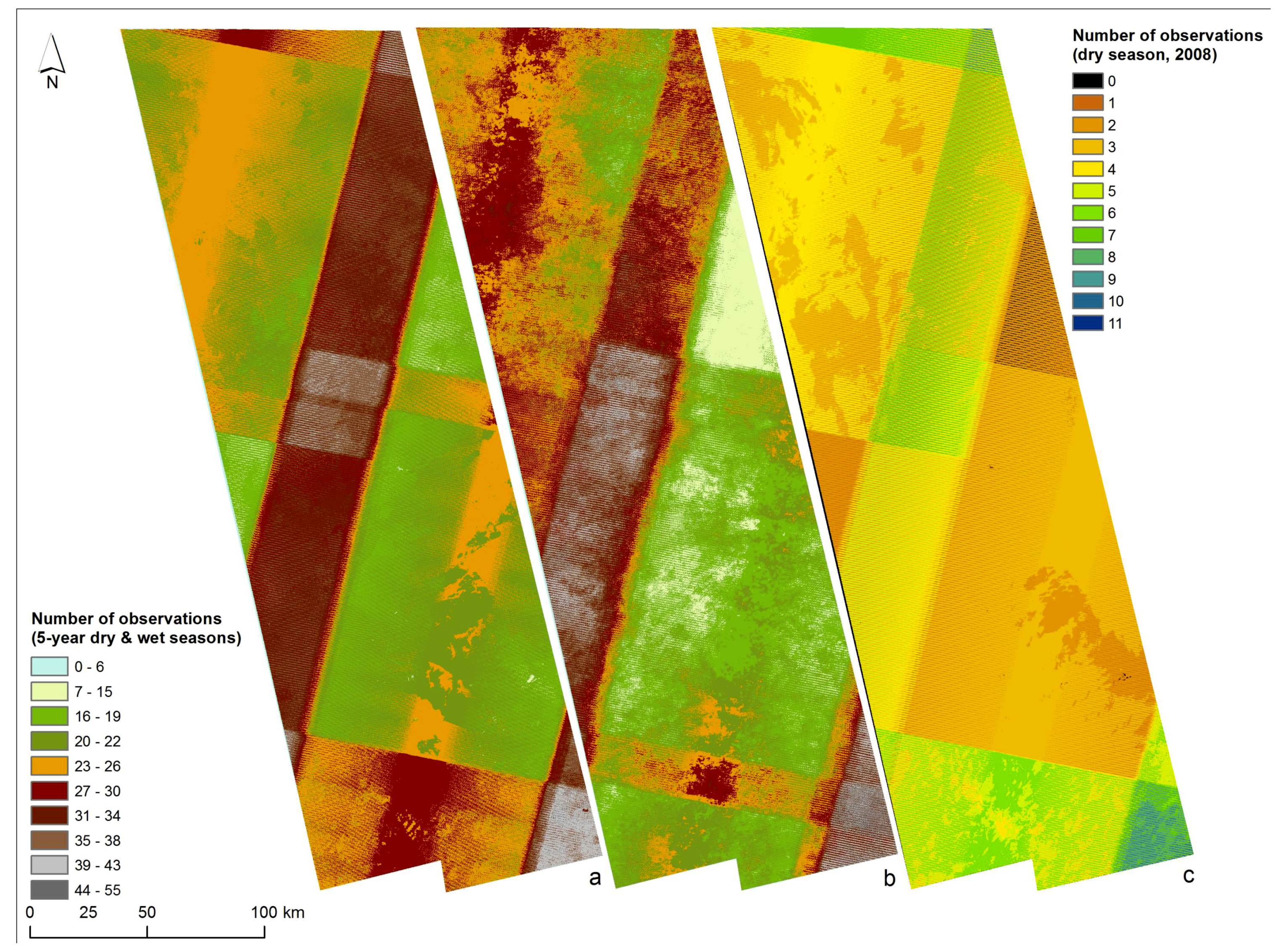
Figure 4.
The overall accuracies and confidence intervals for the 15 land cover mapping model combinations tested. n: the number of variables in each model.
Figure 4.
The overall accuracies and confidence intervals for the 15 land cover mapping model combinations tested. n: the number of variables in each model.

Figure 5.
(a) Land cover map from the best performing model of this study (Model#9 in Table 3); (b) error-adjusted area estimates and 95% confidence interval margins for the four land cover classes estimated from the best performing model; and (c) the 2010 high resolution (SPOT 5 and colour infrared aerial photography-based) land cover data of the South African National Geospatial Information (NGI) mapping agency [43]. Locations A, B and C are the example subsets that appear in Figure 7.

Figure 6.
The class-level accuracy statistics for the 15 models tested.

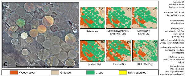
Figure 7.
Example subsets from the study area depicting: (A–C): the aerial imagery; (A1,B1,C1): the NGI 2010 land cover map [43]; and (A2–A6,B2–B6,C2–C6): classification model results of this study.
Figure 7.
Example subsets from the study area depicting: (A–C): the aerial imagery; (A1,B1,C1): the NGI 2010 land cover map [43]; and (A2–A6,B2–B6,C2–C6): classification model results of this study.

Table 1.
Number of Landsat images used in each period for variability metric calculations.
| Period | Start Date | End Date | Landsat 5 (TM) Scenes | Landsat 7 (ETM+) Scenes | L5 + L7 | Total # of Images Used |
|---|---|---|---|---|---|---|
| Dry | 02-6-2006 | 1-10-2006 | 35 | 29 | 64 | |
| 02-6-2007 | 1-10-2007 | 28 | 29 | 57 | ||
| 02-6-2008 | 1-10-2008 | 8 | 29 | 37 | ||
| 02-6-2009 | 1-10-2009 | 0 | 24 | 24 | ||
| 02-6-2010 | 1-10-2010 | 0 | 17 | 17 | Total Dry: 199 | |
| Wet | 01-1-2006 | 01-4-2006 | 5 | 19 | 24 | |
| 21-11-2006 | 31-3-2007 | 30 | 72 | 102 | ||
| 21-11-2007 | 31-3-2008 | 47 | 79 | 126 | ||
| 21-11-2008 | 31-3-2009 | 29 | 83 | 112 | ||
| 21-11-2009 | 31-3-2010 | 5 | 90 | 95 | ||
| 21-11-2010 | 31-12-2010 | 0 | 8 | 8 | Total Wet: 467 | |
| Total Dry + Wet: 666 | ||||||
TM: Thematic Mapper. ETM: Enhanced Thematic Mapper.
Table 2.
Acquisition dates and polarizations for Advanced Land Observing Satellite Phased Array type L-band Synthetic Aperture Radar-1 (ALOS PALSAR-1) data used. FBS: Fine Beam Single polarization; FBD: Fine Beam Dual polarization.
Table 2.
Acquisition dates and polarizations for Advanced Land Observing Satellite Phased Array type L-band Synthetic Aperture Radar-1 (ALOS PALSAR-1) data used. FBS: Fine Beam Single polarization; FBD: Fine Beam Dual polarization.
| Polarization | Path | Frames | Date |
|---|---|---|---|
| FBS | 600 | 6610, 6620, 6630, 6640,6650, 6660 | 14-2-2008 |
| FBS | 600 | 6610, 6620, 6630, 6640,6650, 6660 | 2-3-2008 |
| FBD | 601 | 6610, 6620, 6630, 6640,6650, 6660 | 1-7-2008 |
| FBD | 601 | 6610, 6620, 6630, 6640,6650, 6660 | 18-7-2008 |
Table 3.
The 15 independent models tested in this study and the number of parameters in each.
| Model # | Parameters Included | Number of Parameters |
|---|---|---|
| 1 | Dry Landsat All SAR | 95 |
| 2 | Dry Landsat Dry SAR | 80 |
| 3 | Dry Landsat Wet SAR | 50 |
| 4 | Dry Landsat | 35 |
| 5 | Wet Landsat All SAR | 95 |
| 6 | Wet Landsat Dry SAR | 80 |
| 7 | Wet Landsat Wet SAR | 50 |
| 8 | Wet Landsat | 35 |
| 9 | All Landsat All SAR | 130 |
| 10 | All Landsat Dry SAR | 115 |
| 11 | All Landsat Wet SAR | 85 |
| 12 | All Landsat | 70 |
| 13 | SAR All | 60 |
| 14 | SAR Dry | 45 |
| 15 | SAR Wet | 15 |
Table 4.
Confusion matrix and accuracy statistics for the all-parameter model (Model #9 in Table 3).
Table 4.
Confusion matrix and accuracy statistics for the all-parameter model (Model #9 in Table 3).
| Reference | User’s Accuracy | ||||||
|---|---|---|---|---|---|---|---|
| WV | G | C | NV | Total | |||
| Mapped | Woody vegetation (WV) | 475 | 3 | 1 | 5 | 484 | 0.98 |
| Grassland (G) | 9 | 295 | 15 | 4 | 323 | 0.91 | |
| Cropland (C) | 1 | 33 | 131 | 0 | 165 | 0.79 | |
| Non-vegetated (NV) | 32 | 4 | 0 | 74 | 110 | 0.67 | |
| Total | 517 | 335 | 147 | 83 | 1082 | ||
| Producer’s accuracy | 0.94 | 0.90 | 0.88 | 0.85 | |||
© 2018 by the authors. Licensee MDPI, Basel, Switzerland. This article is an open access article distributed under the terms and conditions of the Creative Commons Attribution (CC BY) license (http://creativecommons.org/licenses/by/4.0/).
Share and Cite
MDPI and ACS Style
Symeonakis, E.; Higginbottom, T.P.; Petroulaki, K.; Rabe, A. Optimisation of Savannah Land Cover Characterisation with Optical and SAR Data. Remote Sens. 2018, 10, 499. https://doi.org/10.3390/rs10040499
AMA Style
Symeonakis E, Higginbottom TP, Petroulaki K, Rabe A. Optimisation of Savannah Land Cover Characterisation with Optical and SAR Data. Remote Sensing. 2018; 10(4):499. https://doi.org/10.3390/rs10040499
Chicago/Turabian StyleSymeonakis, Elias, Thomas P. Higginbottom, Kyriaki Petroulaki, and Andreas Rabe. 2018. "Optimisation of Savannah Land Cover Characterisation with Optical and SAR Data" Remote Sensing 10, no. 4: 499. https://doi.org/10.3390/rs10040499
Note that from the first issue of 2016, this journal uses article numbers instead of page numbers. See further details here.