Article

Automatic Ship Classification from Optical Aerial Images with Convolutional Neural Networks

1
Pattern Recognition and Artificial Intelligence Group, Department of Software and Computing Systems, University of Alicante, 03690 Alicante, Spain
2
Automation, Robotics and Computer Vision Group, Department of Physics, Systems Engineering and Signal Theory, University of Alicante, 03690 Alicante, Spain
*
Author to whom correspondence should be addressed.
Remote Sens. 2018, 10(4), 511; https://doi.org/10.3390/rs10040511
Submission received: 22 February 2018 / Revised: 14 March 2018 / Accepted: 21 March 2018 / Published: 24 March 2018
(This article belongs to the Section Remote Sensing Image Processing)

Abstract

:
The automatic classification of ships from aerial images is a considerable challenge. Previous works have usually applied image processing and computer vision techniques to extract meaningful features from visible spectrum images in order to use them as the input for traditional supervised classifiers. We present a method for determining if an aerial image of visible spectrum contains a ship or not. The proposed architecture is based on Convolutional Neural Networks (CNN), and it combines neural codes extracted from a CNN with a k-Nearest Neighbor method so as to improve performance. The kNN results are compared to those obtained with the CNN Softmax output. Several CNN models have been configured and evaluated in order to seek the best hyperparameters, and the most suitable setting for this task was found by using transfer learning at different levels. A new dataset (named MASATI) composed of aerial imagery with more than 6000 samples has also been created to train and evaluate our architecture. The experimentation shows a success rate of over 99% for our approach, in contrast with the 79% obtained with traditional methods in classification of ship images, also outperforming other methods based on CNNs. A dataset of images (MWPU VHR-10) used in previous works was additionally used to evaluate the proposed approach. Our best setup achieves a success ratio of 86% with these data, significantly outperforming previous state-of-the-art ship classification methods.

Graphical Abstract

1. Introduction

Automatic ship classification has been an active research field for decades and continues to attract increasing interest. These systems are important for maritime surveillance and can be used to monitor marine traffic, illegal fishing and sea border activities, among others. What is more, the rapid growth of remote sensing technologies has a positive effect on many applications such as surveillance and security systems, illegal smuggling and the control of pollution, spills or oil slicks. A wide variety of sensors are commonly used for these tasks, including the Automated Identification System (AIS), the Vessel Monitoring System (VMS), and the Synthetic Aperture Radar (SAR), images in a visible spectrum, as well as hyperspectral imaging acquired by Earth Observation Satellites (EOS).
AIS and VMS use both Very High Frequency (VHF) and Global Positioning System (GPS) to wirelessly transmit the identity and current location of a ship. However, not all the ships are obliged to carry transponders, and sometimes they are intentionally turned off to avoid radar detection. Remote sensing analysis techniques can, therefore, be used in those situations.
The Synthetic Aperture Radar (SAR) uses radar signals to obtain remote sensing imagery. Unlike the visible spectrum, radar signals are affected by neither changes in lighting (day or night) nor weather conditions (clear or cloudy). Nevertheless, SAR images have some limitations depending on the type of SAR, its radiometric and spectral resolution (which is usually quite low), along with the materials and the geometry of the objects to be detected.
On the one hand, optical images have a higher spatial resolution than most SARs, and this fact helps to improve detection and recognition. On the other, AIS or VMS can identify the ship detected, and its absence may be indicative of a ship performing illegal activities or that it is another kind of floating object. The technical advances of visible spectrum sensors have made it possible to obtain images with more spatial resolution than those obtained with SAR. In contrast to SAR, many satellites are equipped with them, such as SPOT, RedEye, LandSat, QuickBird, and CBERS, among others. The main drawback of using visible optical imagery is that they cannot be used at night or under adverse weather conditions.
Automatic ship classification with SAR has been widely studied, and was most recently reviewed in [1,2,3]. When compared to the large amount of feasibility analyses for ship classification based on SAR, far fewer research studies use optical imagery for the same purpose [2]. The advances of optical sensors have made it possible to partly overcome the shortcomings of SAR-based approaches. The proposed work consequently focuses on researching how to improve the accuracy of the classification process while the requirements of real-time ship monitoring are accomplished.
We present a new approach based on Convolutional Neural Networks (CNN) for the automatic classification of ships and small Unidentified Floating Objects (UFOs) from optical aerial imagery acquired in the visible spectrum. CNNs have obtained state-of-the-art results in image classification tasks [4] that are similar to the problem addressed in this work. We propose a CNN architecture adapted to aerial image classification of ships. CNNs are able to identify the most distinctive features for the task at hand avoiding the use of hand-engineered features. The proposed method is evaluated with different topologies frequently used for image classification in literature, and also compared to other conventional machine learning techniques that use well-known features extracted from the images by means of both signal and image processing methods. The proposed method has also been applied to the classification of images acquired from different satellites in order to assess its robustness and generalization. This approach classifies ships in portions (224 × 224 pixels) of satellite images, although it could also be applied to larger images using a sliding window. In this sense, it could be considered that it performs a detection with the precision of the window size.
Another contribution of this work is a dataset of optical aerial images that contains more than 6000 samples correctly labeled and classified into seven classes. To the best of our knowledge, no similar public domain datasets have appeared in literature to date, as previous works use smaller databases for evaluation (a maximum of 400 samples).
In summary, the main contributions of this work are:
  • A learning-driven architecture for detecting if an aerial image contains a ship or not, trained to detect these type of objects in a generic way. In order to improve the performance, the proposed architecture uses a CNN for extracting features (neural codes) which are eventually classified using a kNN algorithm. Different fine-tuning strategies have also been evaluated for training several CNN models.
  • A comparison between the proposed architecture, classical and state-of-the-art works, including some of the most common CNN topologies. The proposed method outperforms the performance of previous approaches, both using a reference database and the dataset compiled in this work.
  • A dataset (MASATI) freely available for download with more than 6000 optical aerial images properly labeled.
The remainder of this paper is organized as follows. The following section provides a brief review of state of the art automatic ship classification methods, with optical aerial images acquired from satellites. Section 3 shows a brief introduction to deep learning and particularly to CNN. Section 4 describes the proposed method, the different CNN architectures that we have evaluated, and the new dataset of images collected and labeled for the appraisal of the classification process. Our experiments are shown in Section 5, in which a comprehensive study of all the models considered is performed. Finally, our conclusions and future work are described in Section 6.

2. Related Work

Automatic classification and detection of ships is a challenging task owing to weather variability (clouds, rain, wind), the natural variability in the surface of the sea (waves), the shape and size of the targets to be recognized, and the presence of natural elements, such as islets, rocks, sandbanks or coral reefs. Previous research on automatic ship recognition from spaceborne optical images has allowed us to establish a baseline framework and a starting point from which to compare and contrast our approach.
Lure and Rau [5] and Weiss et al. [6] proposed a detection system for the tracking of ships that is based on Advanced Very High Resolution Radiometer (AVHR) imagery, in which a preprocessing stage was implemented to extract image features that are later classified with a neural network or directly using similarity measures from features. This system is only able to detect ships in motion as it is based on tracking methods.
The work by Corbane et al. [7] was focused on the detection of small ships in tropical areas using SPOT-5 satellite imagery. This algorithm uses an initial segmentation process by means of adaptive thresholding. A morphological opening operation is then performed to remove noise, and an additional segmentation process based on region-growing is applied to locate candidate ship targets in the image. Finally, these candidate targets are characterized by spectral, shape and textural properties that are utilized as features to train a neural network. In a later work, Corbane et al. [8] introduced a complete processing chain for ship detection using optical satellite imagery in which the aforementioned method [7] was improved, although it also used a preprocessing stage for feature extraction.
More recently, and along the same line, Zhu et al. [9] presented an algorithm in which multiple high-dimensional local features (such as shape and texture) were extracted from potential ship targets and used for classification by employing Support Vector Machines (SVM). Bi et al. [10] described a hierarchical salient-region based algorithm in which features extracted from detected regions were used to train an SVM classifier to detect ships. Xia et al. [11] proposed a method which performs a sea-land segmentation process integrating Local Binary Patterns (LBP) features to use them with a SVM classifier for ship detection. The work by Yang et al. [12] is based on a sea surface homogeneity analysis in which the authors defined a linear function in order to combine computed features from extracted regions so as to select candidate ships. Marques et al. [13] presented an algorithm for vessel detection in aerial image sequences acquired by a sensor mounted on a UAV. The method performs a blob extraction and then applies a process based on the spatial and temporal feature analysis of blobs for their classification in regions of ships or non-ships. A year later, Yang et al. [14] proposed a new approach for the same purpose, in which a visual search engine was designed in order to obtain salient regions using a global contrast model in which both the geometric properties of these regions and the neighborhood similarity are jointly used to discriminate candidate ships. In the last step of this approach, an SVM was used for classification. Tang et al. [15] used wavelet coefficients extracted from the JPEG2000 compressed domain combined with deep (non-convolutional) neural networks and the Extreme Learning Machine. In the initial stage, the input image is preprocessed using both an image enhancement technique and a sea-land segmentation process from the wavelet coefficients, thus setting a criterion for the ship location. In another recent work [16], CNNs were used to extract features which are fed to a region proposal network (RPN) to obtain the precise location of the ship.
As can be seen above, most previous works use similar approaches, i.e., they usually include three stages. First, an initial image pre-processing is implemented to enhance the input image. Next, a set of features carefully hand-crafted or learned for the target task are extracted. Finally, a classification process based on raw features or a supervised learning classifier is performed, generally using SVM [9,10,11,14,17], neural networks [5,7,15], and more recently combining both techniques as in [18], which uses a CNN with an SVM classifier. Sometimes, the input of CNN are not the images acquired but models built using features obtained by combining image processing operations such as denoising, color and line segmentations, and saliency methods as in [19].
Recently, Cheng and Han [20] presented a review concerning target detection methods in optical remote sensing images in which targets were instances of any man-made object. Moreover, they discussed new challenges and proposed new research directions based on deep learning techniques.
A well-known limitation of conventional machine learning techniques is that they are not suitable for dealing with the source image pixels directly, as is discussed in [21]. The adequate extraction and selection of features are crucial steps for detection and classification methods.
In this last year, deep neural networks (in particular, CNN) have been applied for ship detection and classification. Zou and Shi [18] proposed the SVD-Network as a method based on a CNN with two layers to obtain feature maps and a third layer to determine ship a probability map of ship pixels. Later, the authors used the obtained hash maps as inputs of a linear SVM classifier. That proposal was tested using scenes obtained from VRSS-1 and GaoFen-1 satellites, where the half of each satellite were used for training. Lin et al. [22] used a modification of ResNet for classification and localization of inshore ships in a harbor where the targets can present problems as is closely docked side by side. It was tested with a dataset obtained from Google Earth and from GaoFen-2.
In general, previous approaches evaluate their performance using a low number of samples as it happens in [5,6,14], and this complicated the generalization. Sometimes, the experiments are performed with a unique high-resolution scene which is partitioned into non-overlapping sub-images used for training and test as in [23]. In this line, other more recent methods based on deep learning and applied to ship detection, as Lin et al. [22], used 48 different scenes (24 for training) of 5000 × 5000 pixels which are cut in patches extracting image slices obtained many more samples (around 750 samples in this case. There are other works with relatively large datasets, such as [18,19] whose data were collected from Google Earth, but they are not public, making difficult to compare them with other ship classification methods. In contrast to these works, we have collected a dataset composed of more than 6000 images which has been publicly released.
Other problems, such as changes in lighting or weather conditions and images which contain land zones (cost and sea, and not solely sea), are a challenge for traditional approaches because this kind of images usually yields false positives. Many state-of-the-art methods consequently avoid using this kind of input images in their datasets [12,13]. Other methods apply a mask with geographical information in order to ignore land areas [7,10] or separate previously sea and land areas [19], but even in this case there are small islets and islands which are not filtered out and may be detected as UFOs. Moreover, this solution is only valid if used with satellite images, but other sources such as systems mounted on aircraft would need to apply a set of transformations to attain the exact location in which the images were acquired. This last issue implies a loss of precision and the generation of errors. Again, it should be noted that, according to the survey in Cheng and Han [20], one of the most promising research means to solve these issues is the use of deep learning methods, and our work is an effort in this direction.
To summarize, the main objectives of our proposal are to create a new maritime dataset in order to make the results comparable for future algorithms, and to design a deep learning architecture optimized for ship classification.

3. Deep Learning Background

Deep Learning [4,24,25] is a branch of machine learning that uses neural networks with many layers in order to model high level representations of the input data. These data are fed to the first layer, which applies a transformation and sends the processed data to the next layer, repeating this process until the last layer achieves the results. The transformations applied within the first layers yield low-level features , which for input images could be borders, corners, gradients, and so forth, whereas next layers obtain an increasing high-level representation of the most salient or representative features. A key advantage of deep learning is that there is no hand-engineered feature extraction, the most relevant features being learned from the raw input data. This is usually known as representation learning [21].
There are many deep learning architectures, but those most commonly used for image recognition are Convolutional Neural Networks as they obtain excellent results for this kind of inputs [25]. CNNs are composed of one or more convolutional layers, usually followed by pooling layers [26], with optional fully connected layers on top. Regularization methods such as dropout [27] can also be included. These networks can be trained with a standard backpropagation algorithm [28], which requires a labeled dataset in order to calculate a loss function gradient. This dataset must be large and fairly representative in order to learn generic and discriminant features.
Since the first CNN implemented by LeCun et al. [29], recent networks such as AlexNet [30], GoogleNet [31] and ResNet [32] have afforded a significant breakthrough in image classification.
Some of these network architectures and deep learning techniques focused on remote sensing data have been recently reviewed by Zhu et al. [33]. These architectures are used for object detection and scene classification of remote sensing imagery in categories such as residential, forest, agricultural, etc. For instance, in [34] CNN activations from the last convolutional layer at multiple scales are generated and then encoded into global image features through commonly used encoding approaches in order to feed a classifier. Unlike of work shown in [22], in which only ResNet is used, in our proposal, we evaluated some of the most recent CNN topologies to detect the presence of ships, also using different fine-tuning strategies for training the models. Moreover, in that work, the approach presented is oriented to detect ships in harbor in contrast with our method focused on detecting the presence of both inshore and offshore ships in different kind of scenes. As can be seen in our experimentation, the proposed architecture based on CNN achieves accurate classification rates, thus closing the gap in human-level performance in order to detect the ships.
Summarizing, deep learning techniques allow us to face the technological challenges of the remote sensing field as well as successfully overcome some of the limitations of the techniques of the past, as discussed in Zhang et al. [35] and Ball et al. [36]. With that purpose, we present an architecture that uses CNN for extracting features of aerial imagery which are classified using a kNN algorithm instead of a linear SVM classifier as in [18] and using more than 6000 labeled samples of public access.

4. Methodology

This section details the proposed method for classification scenes with or without ships. First, we introduce the state-of-the-art CNN models which will be evaluated in the results section. Then, the proposed hybrid architecture combining these CNN models with k-Nearest Neighbors (kNN) is described. Finally, we introduce the new dataset of aerial imagery compiled for ship classification.

4.1. Network Topologies

As a general rule, there are no guidelines indicating which network architecture or how many layers and neurons per layer are suitable to find a solution for a given classification problem. The most suitable topology depends on the complexity of the problem to be solved, the size of the dataset, the number of classes and the dimensionality of the data. Intuitively, the more difficult the problem is, the more layers and neurons are required. As explained by Pascanu et al. [37], neural networks with many layers (deep) outperform shallow networks (wide). This is because they can divide the input space into many more independent regions, and the number of partitions is exponentially increased after each layer. However, the computational cost as regards training and validation stages also increases with the number of layers and parameters.
In this work, we have evaluated six CNN topologies, which are representative in the image recognition state-of-the-art. Unlike [34], in which models such as AlexNet [30], VGG-F/M/S or VGG-16/19 [38] were used for scene classification, we have chosen two classic (VGG-16/19) and three recent network models: ResNet [32], Inception V3 [39] and Xception [40], that outperform the classic networks in object recognition tasks. Inception V3 and Xception are improved versions of Googlenet. In addition, we have implemented and tested a simple network topology to obtain baseline results for comparison with the other five models described below. The topologies evaluated are:
  • Baseline Network. This network contains only two convolutional layers followed by Max Pooling [30] and Dropout filters [27], and two fully-connected layers at the end. All activation functions are ReLU [41]. A detailed description is shown in Table 1.
  • VGG-16 and VGG-19 [38]. VGG-16 has 13 convolutional and three fully-connected layers, whereas VGG-19 is composed of 16 convolutional and three fully-connected layers. Both topologies use Dropout and Max-pooling techniques and ReLU activation functions.
  • Inception V3 [39]. This architecture has six convolutional layers followed by three Inception modules and a last fully connected layer. It has fewer parameters than other similar models thanks to the Inception modules whose design is based on two main ideas: the approximation of a sparse structure with spatially repeated dense components, and the use of dimensionality reduction to keep the computational complexity in bounds.
  • REsNet [42]. The deep REsidual learning Network learns residual functions with reference to the layer inputs rather than learning unreferenced functions. This technique enables the use of a large number of layers. We have used the 50-layer version for our experimental tests.
  • Xception [40]. This model has 36 convolutional layers with a redesigned version of Inception modules which enable the depthwise separable convolution operation. This architecture outperforms the Inception results using the same number of parameters.
As can be seen in the results section, the Baseline Network model allowed us to perform several initial experiments with various configurations before using more complex topologies. Moreover, it served to obtain a result with a simple model with which to compare the performance. All the network topologies have been evaluated under the same conditions using the architecture shown in the following section.

4.2. Proposed Architecture

As stated in the background section, neural networks are excellent in regards to representation learning. This feature makes them suitable for transfer learning, which consists of applying a model trained for a particular task to a different task [42]. The transfer can be done by fine-tuning the existing weights of the network using the new dataset in order to adjust the model to a new target problem [43], or using the network as a feature extractor, which does not require re-training. In the latter case, an input sample is forwarded in order to obtain an intermediate representation (a vector) from any hidden layer. These vectors are usually called neural codes and can be used as input to other classifiers such as k-Nearest-Neighbors (kNN).
In the proposed architecture, we use this combined approach in order to improve the performance. First, we initialize the network with the pre-trained weights from the ILSVRC dataset (a 1000 classes subset from ImageNet [44], a generic purpose database for object classification), and then we fine-tune these weights using the samples from our dataset (which is presented in the following section). The main advantages of using this technique are that the network can be trained using less data and in addition it converges faster.
The training is carried out by means of standard backpropagation using Stochastic Gradient Descent [45] and considering the adaptive learning rate method proposed by Zeiler [46]. In the backpropagation algorithm, categorical crossentropy has been used as the loss function between the CNN output and the expected result. The training lasted a maximum of 500 epochs with early stopping when the loss did not decrease during 10 epochs. The mini-batch size was set to 32 samples.
Once the network has been trained, we utilize the second type of transfer learning explained above, in which we extract the vectors of characteristics or neural codes (NC) from the training set samples. These NC are used during the inference process to perform the classification of new samples. Given a new sample, it is forwarded through the network to obtain its NC, which is then classified using kNN. As previously explained, this technique is a common practice in transfer learning, although it is usually applied to adapt a model to a different domain (a different dataset), whereas in this work we are applying it to the same domain in order to improve the performance, as shown in the evaluation section (Section 5).
Intuitively, applying kNN on NC achieves better results than the network itself because the network only applies a linear classifier in the last layer (the Softmax operation), remaining with the most similar class. However, kNN is based on finding the sample with the most similar characteristics (NC in this case), so the larger the dataset of samples, the greater the possibility of finding a similar sample.
Figure 1 shows the proposed architecture for classification. There are two stages in this scheme: training and classification. In the first stage, the CNN is trained with standard backpropagation to attain the model weights. After this stage, all the images in the training set are forwarded to obtain their neural codes (NC). In the inference stage, the target image is then also forwarded through the trained CNN in order to calculate its corresponding neural codes, which are compared to those of all the training prototypes using kNN to attain the most likely class of that sample.
In addition, we consider 2 for the normalization of the neural codes. This is a common practice [47,48] in transfer learning. Let x be a vector of size m which represents the neural codes. The 2 normalization is then defined as:
| x | = i = 1 m | x i | 2
The different network topologies described in Section 4.1 are used in the CNN module of the architecture shown in Figure 1. The aim is to empirically compare these topologies in order to obtain the best model in addition to comparing the standard Softmax output (denoted as NC + Softmax in the experiments) with the proposed hybrid approach using kNN with 2 normalization (denoted as NC + 2 + kNN).
In order to fine-tune the evaluated CNNs using the number of classes in our dataset, it was necessary to modify their last layers, replacing the last fully-connected part of the original networks by the three custom layers that can be seen in Table 2. In order to join these layers with the different output sizes of each network, we added a global spatial average pooling layer that allowed us to resize the output dimensionality to the desired size.
The neural codes were obtained from the last hidden layer, which has a size of 1256 (see Table 2). After evaluating several hidden layers and different sizes, the best average results were obtained using the last hidden layer with the indicated size and, therefore, this setting was selected for the following experiments. In this layer is where the highest level features can be found, allowing to make a better grouping of data by class, and therefore obtaining better results when looking for similar prototypes.

4.3. MASATI Dataset

To the best of our knowledge, the only public dataset labeled for classification of scenes with ships and with a sufficient number of images is MWPU VHR-10 [49], which is a general purpose collection containing 800 samples classified into 10 classes, and only 302 ships distributed throughout 57 images. We have used this dataset to compare the results of our approach with previous methods evaluated with the same data.
The size of the dataset is crucial for good CNN training as a consequence of the large number of parameters to be learned. It is additionally important to have sufficient representative samples for each class in order to avoid overfitting and obtain generic and discriminant features. We have, therefore, created a dataset denominated as MASATI (Maritime SATellite Imagery) that contains 6212 satellite images in the visible spectrum which were obtained from Microsoft Bing maps.
In this dataset, each image has been manually labeled according to the following seven classes: land, coast, sea, ship, multi, coast-ship and detail. Table 3 shows the sample distribution of each class. The ship sub-class represents images where a single ship appears within the image. The multi sub-class describes other images in which two ore more instances of ships appear within them. In both sub-classes, the ships have lengths between 4 and 10 pixels. Also, the coast and ship sub-class represents images with one ship close to coast with similar dimensions to the two classes mentioned before and detail sub-class are images with a single ship with a length between 20 and 100 pixels. The images were captured in RGB and with different sizes, inasmuch as the size is dependent on the region of interest to be registered in the image. In general, the average image size has a spatial resolution around 512 × 512 pixels. The dataset was compiled between March and September of 2016 from different regions in Europe, Africa, Asia, the Mediterranean Sea and the Atlantic and Pacific Oceans.
As mentioned previously, methods for automatic ship classification from optical imagery are affected by many factors such as lighting or weather conditions. The proposed dataset therefore considers a great variability of possible situations, thus enabling the proposed CNN approaches to obtain generic features. Figure 2 shows some examples of the images in our dataset. The MASATI dataset is available for the scientific community on demand at http://www.iuii.ua.es/datasets/masati.

5. Experiments

This section provides details on the results obtained after carrying out experiments with which to appraise our method. First, the dataset configuration and the data augmentation process is described in Section 5.1. The evaluation metrics are then defined in Section 5.2, after which the methodology used to tune the CNN hyperparameters is detailed in Section 5.3. In Section 5.4, the proposed approach is evaluated using the MASATI dataset, and the results are compared with those of state-of-the-art methods. Finally, Section 5.5 details the experiments with another dataset (MWPU VHR-10) that has been used to compare our best approach with those of other previous works.

5.1. Dataset Configuration

Our approach was principally assessed using the MASATI dataset described in Section 4.3. In order to measure how the complexity of the dataset, according to the number of classes, impacts on the classification process, three sets were created by grouping samples of different classes as follows:
Set 1 = { Ship , Sea } Set 2 = Set 1 { Coast & Ship , Coast } Set 3 = Set 2 { Detail , Multi , Land }
We evaluated these sets considering both the main class (which only distinguishes between ships or non-ships), and the sub-class (the fine grain labels, see Table 3). Therefore, we performed a total of five experiments, one for Set 1, whose main and sub-class labels are the same, and two for each of both Sets 2 and 3.
In all the experiments, we used a n-fold cross validation (with n = 5 ), which yields a better Monte-Carlo estimate than when solely performing the tests in a single random partition [50]. Our dataset was consequently divided into n mutually exclusive sub-sets, maintaining the percentage of samples for each class. For each fold, we used one of the partitions for test ( 20 % of samples) and the rest for training ( 80 % ). The classifier was trained n times using these sets, after which the average results were calculated.
Before training, the raw input data were initialized by a zero-mean of a z-score normalization [51]:
Z = M m e a n ( M ) s t d ( M )
where M is the input matrix containing the raw image pixels from the training subset. The same operation was subsequently applied to the test subset, maintaining the same mean and standard deviation calculated for the training. The z-score normalization satisfied the standard normal distribution, i.e., each of the dimensional data had a zero mean and standard deviation. This helped correct outliers and remove the effect of lighting, thus improving the performance.
In this work, we have applied data augmentation [30,52] in order to artificially increase the size of the training subset by adding certain random transformations (concretely translation, rotation and reflection) to the input data in order to generate new samples. This technique usually improves the performance and helps reduce overfitting.

5.2. Evaluation Metrics

In order to evaluate the performance of the proposed models, two evaluation metrics widely used for this kind of tasks were chosen: F-measure ( F 1 ) and Average Precision (AP). F 1 can be defined by means of precision and recall:
Precision = T P T P + F P Recall = T P T P + F N F - measure = 2 · Precision · Recall Precision + Recall
where TP (True Positives) denotes the number of correctly detected ships, FN (False Negatives) the number of non-detected or missed ships, and FP (False Positives or false alarms) the number of incorrectly detected ships.
The Average Precision (AP) metric has been used to compare the behavior of our method with that of others, in terms of the ship classification ratio. AP calculates the mean precision value in the recall interval [ 0 , 1 ] , which is equivalent to the area under the Precision-Recall Curve (PRC). It is not, therefore, necessary to represent the PRC in order to show the performance.
Since both datasets contain classes that are unbalanced such as the MASATI classes Multi and Coast & ship, we have chosen these metrics rather than the accuracy or other alternatives, as they are more appropriate and fairer in the case of unbalanced data. In addition, for the case of classification using sub-classes, we calculate the confusion matrix in order to analyze the errors.

5.3. Hyperparameters Evaluation

Both size and image quality may have an impact on the performance of the deep learning techniques used, as mentioned in [53,
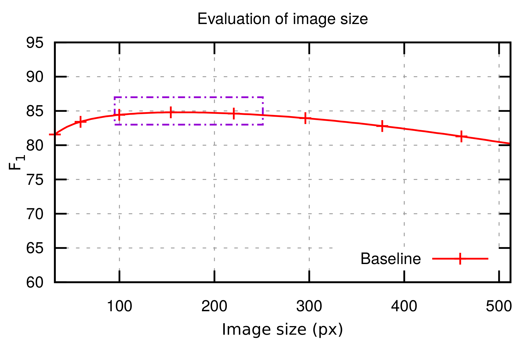
54]. In order to determine how the image size could affect our models, we performed exhaustive experimentation by means of rescaling the input images to sizes ranging from 32 × 32 pixels to 512 × 512 pixels using an anisotropic scaling. This scaling was used rather than square crop because cropping may remove information that is relevant to our task, such as ships that are close to the image borders.
Figure 3 shows the average F 1 score obtained for the Set 3 and the main class labeling, using the network model described in Table 1. We performed this experiment using only the Baseline network because the other models have a fixed input size due to their architecture limitations. As can be seen in this plot, changing the size of the image makes the F 1 to vary up to 5 %, and the optimal results are obtained with image sizes ranging from 100 × 100 pixels to 250 × 250 pixels. This experiment allows us to verify that the optimal range of input size matches that of the other CNN topologies evaluated, which is set to 224 × 224 pixels.
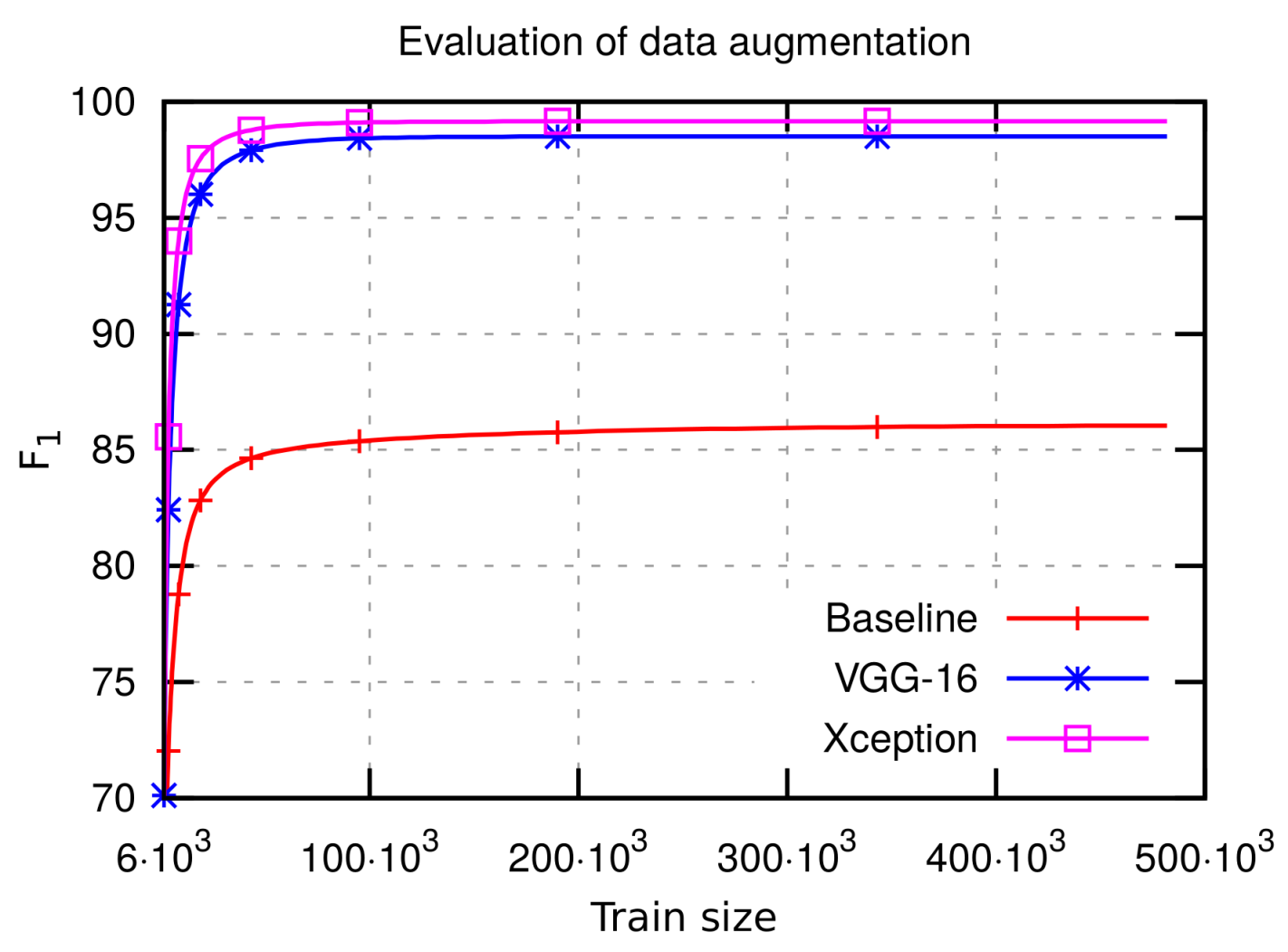
Furthermore, as previously mentioned, some images underwent transformations in order to generate new data and increase the training dataset. Data augmentation increases the performance when using our baseline CNN and the MASATI dataset, as shown in Figure 4. This plot shows the positive impact of data augmentation in the F 1 , which increases until stability is attained. This experiment was also done with Set 3 and the main class labeling. In addition to the baseline network, we evaluated other two models, VGG-16 and Xception, which are those that obtained better results. The highest increase occurs at the beginning, when around five and 10 new samples are generated from each image in the original dataset. Although a higher F 1 can be obtained by adding many augmented samples, we set this parameter to 5 for the subsequent experiments, as a high number of samples also significantly increases the computation cost during the training stage. All these experimental tests allowed us to adjust the training parameters for the CNNs topologies evaluated in the following section.

5.4. Results with MASATI Dataset

This section shows the evaluation of the six CNN topologies described in Section 4.1. Training was carried out in three different ways for each network: Final (backpropagating from only the last three layers, which are fully connected), Middle (backpropagating from the second half of the network), and Full (training the whole network). In all three cases, weights were initialized using a model pre-trained with ILSVRC ImageNet [44] in order to subsequently perform fine-tuning. The only exception was the baseline network, which was only trained without initialization and using the Full approach, since being a custom model it could not have pre-trained weights.
In order to adjust the kNN classification of our architecture, five values of k = {1, 5, 10, 15, 20} were tested. We evaluated incremental values of k until a downward trend was obtained, selecting that which obtained the highest F 1 . The best k was, on average, 8 . 84 using 2 -normalized neural codes. Therefore, a value k = 10 was chosen, since it is the closest value of k.
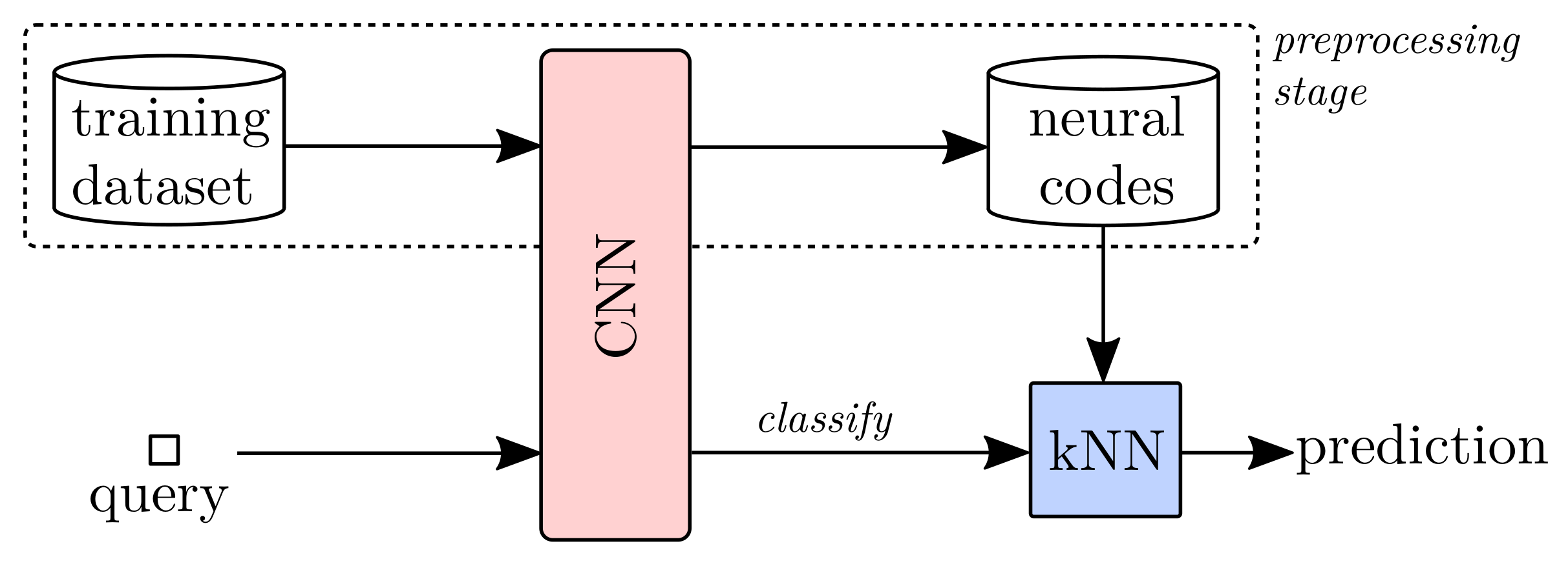
The results obtained when using the standard Softmax output on the neural codes are reported for each network model and training method (NC + Softmax), along with the proposed architecture (NC + 2 + kNN). Table 4 and Table 5 show a comparison of the results contained in the three sets described in Section 5.1 using all network models and architecture configurations, along with the three types of fine-tuning.
Table 4 shows the results obtained using the main class labeling (Ship/Non-ship). To perform this evaluation, we trained the CNN using only two classes and then we obtained the neural codes. During classification, evaluation was performed using both Softmax, and kNN search on the training set prototypes. Table 5 shows the results using the same methodology above, but in this case the models were trained and evaluated with the seven sub-classes. Table 5 does not include the results for Set 1 as they are the same as shown in Table 4 (this set only includes Ship and Non-ship labels). In both tables, the value displayed is the F 1 percentage for the average of the 5 folds. The best result for each model and set is shown in bold type. The lower rows show the average of all models for each set, and also for all sets, excluding the base network since it can only contribute to one average, therefore it would bias those data.
As can be seen in Table 4 and Table 5, the best average results for all models are obtained with NC + 2 + kNN and full training. The Xception model specifically yields the highest score for the three sets, closely followed by VGG-16, REsNet, and Inception V3. As can be noted, the fine-tuning configuration also has an impact on the F 1 . On average, the middle training outperforms final training, and the full training is better than the middle and final training.
To analyze this hypothesis in a more rigorous way, we performed a statistical significance analysis by considering the non-parametric Wilcoxon signed-rank test [55]. More precisely, the idea is to assess whether the improvement observed in the classification performance with the use of the NC + 2 + kNN is statistically relevant. For this we compared the results obtained with both approaches (NC + Softmax and NC + 2 + kNN) in each of the five-folds, with all the network models, the three types of training, the three sets evaluated, and both the main and the sub-class level. The results showed that the proposed method (NC + 2 + kNN) significantly improved the NC + Softmax approach considering a statistical significance threshold of p < 0 . 01 (the most restrictive threshold normally used).
Previous experiments showed that adding weight initialization increases the F 1 by 4.5% on average. Therefore, it is expected that using this technique on the baseline model could increase its performance similarly, although it would be still far from the state-of-the-art models evaluated. As shown in Figure 4, adding more training images helps improving the F 1 until a limit is reached, from which the models do not seem to improve further. This indicates that the obtained results are also very dependent of the network architecture used. For example, for classifying the Sets 1 and 2 there is a difference of more than a 10% between VGG-16 and Xception, both using weight initialization.
Table 4 and Table 5 show that the best average results were obtained with Set 3, which can be explained because it is the one with a larger number of samples. However, results using Set 2 are slightly lower than those from Set 1, maybe due to the addition of two new classes that are unbalanced (Coast and Coast & Ship). Additionally, Set 3 contains more classes with many more samples of ship and land (more than 3000 new samples are added), allowing a better discrimination.
Besides, there is a difference in F 1 between the average results obtained when classifying the main classes (Table 4) and the sub-classes (Table 5). Note that the average result obtained with the sub-classes increases for Set 2 and decreases for Set 3, although if we compare the results of the best model (Xception) then an improvement is observed in both cases. This improvement when performing the classification using the sub-classes (which although it has more classes obtains better results) may be due to the fact that certain classes are confused when grouping them into Ship or Non-ship, such as Coast and Coast & Ship.
In order to analyze these errors, we visualize them using confusion matrices. 
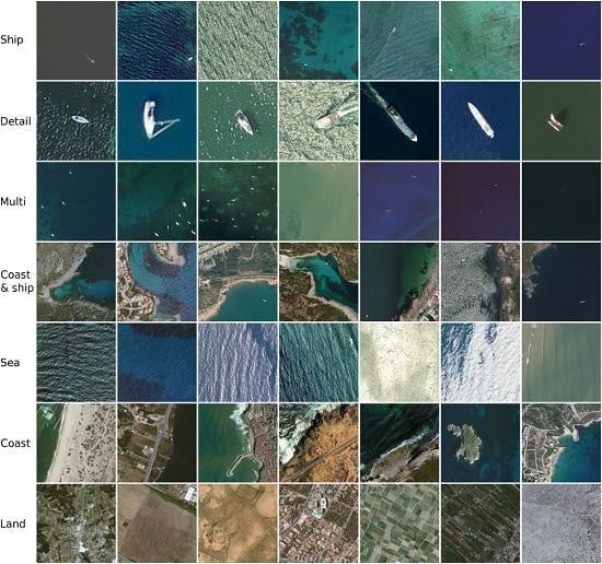
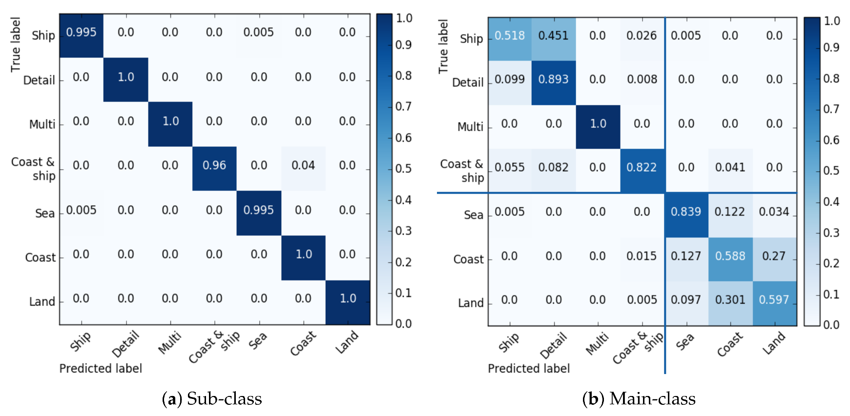
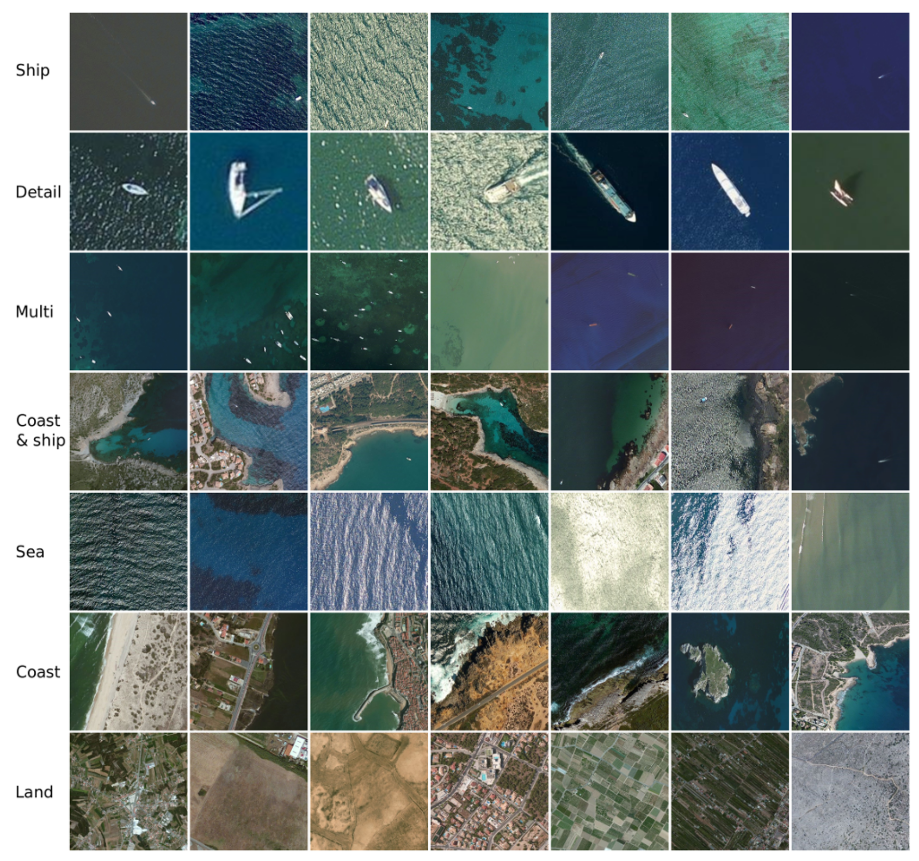
Figure 5a shows the normalized confusion matrix for sub-classes. It can be seen that most instances are correctly classified, and the errors are only caused by confusion between Ship and Sea, as well as between Coast and Coast & Ship. As can be seen in Figure 2, Ship and Sea samples are very similar since, in general, the size of the ships is very small and it could cause a bad classification. The same occurs with Coast and Coast & Ship classes.
Figure 5b shows the normalized confusion matrix for the main-class classification, but analyzed at the sub-class level. That is, in this case the system was trained and evaluated at the main-class level, but we generated the confusion matrix by assessing the error using the sub-class to which it would belong. It can be seen that although it is trained to differentiate between the main classes, the network learned discriminative characteristics that allows it to differentiate the ships also within the sub-class level.
It can be seen that the main mistakes are made within the main-class group (separated in quadrants by two blue lines in the graph), for example when classifying Ship samples as Detail, or Coast samples as Land. Much fewer errors are made between the main classes, where only some samples of Sea and Ship, and Coast and Coast & Ship are confused.
In addition to the experiments shown in Table 4 and Table 5, which prove both the validity and the robustness of our proposal, we also compared it with other methods used for ship classification. Table 6 shows a comparison of our best architecture (Xception NC + 2 + kNN) and some traditional techniques mentioned in Section 3. These experiments were done using the MASATI dataset and the main class labeling to discriminate the occurrence of ships. Specifically, the techniques with which we compare our method are:
  • “Features + NN”: An approach that is similar to the method described in [7], which is based on hand-crafted features, was evaluated. This algorithm applies an adaptive threshold and a morphological opening (with a kernel of 2 × 2) to remove noise. The candidate ships are located by means of a region-growing process. These objects are characterized by a set of features which are used to train a neural network (a fully-connected network with three hidden layers and four nodes in each layer).
  • “HOG + SVM”: An approach with which to extract local features from the input images that is based on the methods proposed in [9,10,11]. This algorithm calculates the Histogram of Oriented Gradients (HOG) [56] (with a 8 × 8 cell size, a 16 × 16 block size, and nine histogram channels) and classifies them using SVM (using the C-Support Vector implementation with a penalty parameter of C = 100 ). HOG is based on the counting occurrences of gradient orientation in localized portions of an input image.
  • “ORB + aNN”: This method uses the Oriented FAST and rotated BRIEF (ORB) [57] (with an edge threshold of 10, a patch size of 31, a scale factor of 1.2, and eight levels in the scale pyramid) to extract local features that are paired using an approximate Nearest Neighbors (aNN) algorithm. For this step we evaluated different values of k (up to k = 20 ), finally determining that k = 2 obtained the best results. ORB is a fast robust local feature detector based on the FAST keypoint detector and on the BRIEF (Binary Robust Independent Elementary Features) visual descriptor, and includes some modifications to enhance the performance.
According to the results of the comparison shown in Table 6, it is possible to affirm that, taken the ground truth of our dataset, our best approach (Xception NC normalized with 2 and using a kNN) outperforms the best result of any other previous method, attaining a F 1 score of 99.05% versus 79.27% for ‘HOG + SVM” (the best of the traditional methods).

5.5. Results with MWPU VHR-10 Dataset

The evaluation has also been performed with an existing dataset used for aerial scenes classification in literature, in order to compare the score of our best setup with other approaches that had previously been evaluated with these data. MWPU VHR-10 [20,49] is a challenging ten-class geospatial object classification dataset that contains 800 VHR optical remote sensing images gathered from Google Earth. These images are of different sizes, ranging between a spatial resolution of 0.08 to 2 m. They are divided into two sets: a positive set including 650 images, each of which contains at least one target to be detected, and a negative set including 150 images which do not contain any target. The positive set consists of the following classes: 757 airplanes, 302 ships, 655 storage tanks, 390 baseball diamonds, 524 tennis courts, 159 basketball courts, 163 ground track fields, 224 harbors, 124 bridges and 477 vehicles.
The experiments were carried out by organizing this dataset into only two classes: ships (all samples containing vessels) and non-ships (all the other images, including those from the negative set). Table 7 shows a quantitative comparison in terms of the Average Precision (AP) of our architecture using the best CNN approach (Xception) and another five methods from the state of the art:
  • “BOW-SVM” of Xu et al. [58] based on Bag-Of-Words (BOW) feature and SVM classifier.
  • “SSCBOW” of Sun et al. [59] based on Spatial Sparse Coding (SSC) and BOW.
  • “Exemplar-SVMs” of Malisiewicz et al. [60] based on a set of exemplar-based SVMs.
  • “FDDL” of Han et al. [61] based on visual saliency modeling and Fisher Discrimination Dictionary Learning.
  • “COPD” of Cheng et al. [49] based on a collection of part detectors, in which each detector is a linear SVM classifier specialized in the classification of objects or recurring spatial patterns within a certain range of orientation.
The details regarding the implementation and parameters used in these five methods can be found in the work by Cheng et al. [49]. As illustrated in Table 7, our method significantly outperforms all the approaches evaluated in terms of AP for the ship recognition task.
The initialization of our method was performed using the weights learned with the MASATI dataset for the ship/not ship model. Once the model was initialized with these weights, it was trained during 20 epochs. The results in Table 7 are shown initializing the network with these weights and without training (obtaining a 78.12%), and also after the 20 fine-tuning epochs (improving up to 86.02%) without data augmentation. For training and validation with this dataset, we also performed a five-fold cross-validation experiment. Therefore, this dataset was split into five exclusive subsets, maintaining the percentage of samples for each class, and it was trained and validated five times. The reported results are the average performance.
Our method based on NC + 2 + kNN again obtains the best results for ship recognition when retraining the model using this dataset. Even without retraining, the method generalizes well and the average precision is higher than most previous methods. When fine-tuning our network with only 20 epochs and without data augmentation the average precision achieves state-of-the-art results.

6. Conclusions and Future Work

This paper investigates the use of convolutional neural networks for ship classification in aerial images of visible spectrum. We have evaluated our approaches by compiling a dataset of maritime scenes from Microsoft Bing satellite images. The images in this dataset, called MASATI, have been labeled as ships and non-ships, and these classes have subsets containing land, cost or sea. The MASATI dataset has a total of 6212 images of which 3113 contain ships.
We have used this dataset to train different convolutional neural network topologies, which we propose doing through the use of a baseline CNN to adjust the hyperparameters. We then use these hyperparameters to train widely known CNN models, using fine-tuning strategies starting from different layers of the network. The best results are obtained with full training and with Xception network. Our method also performs accurately in maritime scene classification in which the objective is to detect not only a ship or non-ship but also coast, land, sea and multiple instances of a ship.
We also prove that extracting neural codes in order to use them to feed a kNN on inference improves the classification rate, even when the targets are represented by a few pixels in small regions, and independently of the kind of ship (cargo, oil, boat, cruiser, etc.). Different configurations have been evaluated to learn the weights that are used to extract the neural codes on inference. Our best approach (full training an Xception network and extracting normalized neural codes to feed a kNN) clearly outperforms all the state-of-the-art methods when considering average precision and F 1 score.
We additionally carried out another assessment of the proposed architecture in order to prove that it can generalize well. We show that our best approach obtains competitive results even when it is directly applied to a dataset different from that used for training (NWPU VHR-10), and it outperforms the state-of-the-art results in this dataset when the model is fine-tuned for only 20 epochs using these data.
Future research work includes incorporating location features into our classification system in order to obtain the ship position within optical aerial images. Other sensors, such as SAR, could additionally be evaluated for situations in which it is not possible to use visible spectrum imagery, as occurs at night. Different sensors could also be combined in a multimodal scenario. In addition to classifying whether or not an image contains a ship, the exact location of the ship detected could also be extracted by means of saliency estimation methods. We also plan to add more images to the MASATI dataset to make it larger and build better models. In order to speed up this process, semi-supervised strategies [62] could be considered.

Acknowledgments

This work was funded by both the Spanish Government’s Ministry of Economy, Industry and Competitiveness and Babcock MCS Spain through the projects RTC-2014-1863-8 and INAER4-14Y(IDI-20141234).

Author Contributions

Antonio-Javier Gallego designed and performed the experiments; Antonio-Javier Gallego, Antonio Pertusa and Pablo Gil analyzed the data and wrote the paper.

Conflicts of Interest

The authors declare no conflict of interest. The founding sponsors had no role in the design of the study; in the collection, analyses, or interpretation of data; in the writing of the manuscript, and in the decision to publish the results.

References

  1. Crisp, D. The State-of-the-Art in Ship Detection in Synthetic Aperture Radar Imagery; Australian Government, Department of Defense: Canberra, Australia, 2004; p. 115. [Google Scholar]
  2. Greidanus, H.; Kourti, N. Findings of the DECLIMS project—Detection and Classification of Marine Traffic from Space. In Proceedings of the SEASAR 2006: Advances in SAR Oceanography from ENVISAT and ERS Missions, Frascati, Italy, 23–26 January 2006. [Google Scholar]
  3. Marino, A.; Sanjuan-Ferrer, M.J.; Hajnsek, I.; Ouchi, K. Ship Detection with Spectral Analysis of Synthetic Aperture Radar: A Comparison of New and Well-Known Algorithms. Remote Sens. 2015, 7, 5416. [Google Scholar] [CrossRef]
  4. LeCun, Y.; Bengio, Y.; Hinton, G. Deep learning. Nature 2015, 521, 436–444. [Google Scholar] [CrossRef] [PubMed]
  5. Lure, F.Y.M.; Rau, Y.C. Detection of Ship Tracks in AVHRR Cloud Imagery with Neural Networks. In Proceedings of the 1994 IEEE International Geoscience and Remote Sensing Symposium (IGARSS ’94), Pasadena, CA, USA, 8–12 August 1994; pp. 1401–1403. [Google Scholar] [CrossRef]
  6. Weiss, J.; Luo, R.; Welch, R. Automatic detection of ship tracks in satellite imagery. In Proceedings of the IEEE International Geoscience and Remote Sensing (IGARSS ’97), Remote Sensing—A Scientific Vision for Sustainable Development, Singapore, 3–8 August 1997; Volume 1, pp. 160–162. [Google Scholar] [CrossRef]
  7. Corbane, C.; Marre, F.; Petit, M. Using SPOT-5 HRG Data in Panchromatic Mode for Operational Detection of Small Ships in Tropical Area. Sensors 2008, 8, 2959–2973. [Google Scholar] [CrossRef] [PubMed]
  8. Corbane, C.; Najman, L.; Pecoul, E.; Demagistri, L.; Petit, M. A Complete Processing Chain for Ship Detection Using Optical Satellite Imagery. Int. J. Remote Sens. 2010, 31, 5837–5854. [Google Scholar] [CrossRef]
  9. Zhu, C.; Zhou, H.; Wang, R.; Guo, J. A Novel Hierarchical Method of Ship Detection from Spaceborne Optical Image Based on Shape and Texture Features. IEEE Trans. Geosci. Remote Sens. 2010, 48, 3446–3456. [Google Scholar] [CrossRef]
  10. Bi, F.; Liu, F.; Gao, L. A hierarchical salient-region based algorithm for ship detection in remote sensing images. In Lecture Notes in Electrical Engineering; Springer: Berlin/Heidelberg, Germany, 2010; Volume 67, pp. 729–738. [Google Scholar] [CrossRef]
  11. Xia, Y.; Wan, S.; Jin, P.; Yue, L. A Novel Sea-Land Segmentation Algorithm Based on Local Binary Patterns for Ship Detection. Int. J. Signal Process. Image Process. Pattern Recognit. 2014, 7, 237–246. [Google Scholar] [CrossRef]
  12. Yang, G.; Li, B.; Ji, S.; Gao, F.; Xu, Q. Ship Detection From Optical Satellite Images Based on Sea Surface Analysis. IEEE Geosci. Remote Sens. Lett. 2014, 11, 641–645. [Google Scholar] [CrossRef]
  13. Marques, J.S.; Bernardino, A.; Cruz, G.; Bento, M. An algorithm for the detection of vessels in aerial images. In Proceedings of the 2014 11th IEEE International Conference on Advanced Video and Signal Based Surveillance (AVSS), Seoul, Korea, 26–29 August 2014; pp. 295–300. [Google Scholar] [CrossRef]
  14. Yang, F.; Xu, Q.; Gao, F.; Hu, L. Ship detection from optical satellite images based on visual search mechanism. In Proceedings of the 2015 IEEE International Geoscience and Remote Sensing Symposium (IGARSS), Milan, Italy, 26–31 July 2015; pp. 3679–3682. [Google Scholar] [CrossRef]
  15. Tang, J.; Deng, C.; Huang, G.B.; Zhao, B. Compressed-Domain Ship Detection on Spaceborne Optical Image Using Deep Neural Network and Extreme Learning Machine. IEEE Trans. Geosci. Remote Sens. 2015, 53, 1174–1185. [Google Scholar] [CrossRef]
  16. Yao, Y.; Jiang, Z.; Zhang, H.; Zhao, D.; Cai, B. Ship detection in optical remote sensing images based on deep convolutional neural networks. J. Appl. Remote Sens. 2017, 11. [Google Scholar] [CrossRef]
  17. Hu, F.; Xia, G.S.; Wang, Z.; Huang, X.; Zhang, L.; Sun, H. Unsupervised Feature Learning Via Spectral Clustering of Multidimensional Patches for Remotely Sensed Scene Classification. IEEE J. Sel. Top. Appl. Earth Obs. Remote Sens. 2015, 8, 2015–2030. [Google Scholar] [CrossRef]
  18. Zou, Z.; Shi, Z. Ship Detection in Spaceborne Optical Image With SVD Networks. IEEE Trans. Geosci. Remote Sens. 2016, 54, 5832–5845. [Google Scholar] [CrossRef]
  19. Zhang, R.; Yao, J.; Zhang, K.; Feng, C.; Zhang, J. S-CNN Ship Detection from High-Resolution Remote Sensing Images. ISPRS Int. Arch. Photogramm. Remote Sens. Spat. Inf. Sci. 2016, 423–430. [Google Scholar] [CrossRef]
  20. Cheng, G.; Han, J. A survey on object detection in optical remote sensing images. SPRS J. Photogramm. Remote Sens. 2016, 117, 11–28. [Google Scholar] [CrossRef]
  21. Bengio, Y.; Courville, A.; Vincent, P. Representation Learning: A Review and New Perspectives. IEEE Trans. Pattern Anal. Mach. Intell. 2013, 35, 1798–1828. [Google Scholar] [CrossRef] [PubMed]
  22. Lin, H.; Shi, Z.; Zou, Z. Fully Convolutional Network With Task Partitioning for Inshore Ship Detection in Optical Remote Sensing Images. IEEE Geosci. Remote Sens. Lett. 2017, 14, 1665–1669. [Google Scholar] [CrossRef]
  23. Yang, W.; Dai, D.; Triggs, B.; Xia, G.S. SAR-Based Terrain Classification Using Weakly Supervised Hierarchical Markov Aspect Models. IEEE Trans. Image Process. 2012, 21, 4232–4243. [Google Scholar] [CrossRef] [PubMed]
  24. Arel, I.; Rose, D.C.; Karnowski, T.P. Deep Machine Learning—A New Frontier in Artificial Intelligence Research. IEEE Comput. Intell. Mag. 2010, 5, 13–18. [Google Scholar] [CrossRef]
  25. Schmidhuber, J. Deep learning in neural networks: An overview. Neural Netw. 2015, 61, 85–117. [Google Scholar] [CrossRef] [PubMed]
  26. Martinez, H.P.; Bengio, Y.; Yannakakis, G.N. Learning deep physiological models of affect. IEEE Comput. Intell. Mag. 2013, 8, 20–33. [Google Scholar] [CrossRef]
  27. Srivastava, N.; Hinton, G.; Krizhevsky, A.; Sutskever, I.; Salakhutdinov, R. Dropout: A Simple Way to Prevent Neural Networks from Overfitting. J. Mach. Learn. Res. 2014, 15, 1929–1958. [Google Scholar]
  28. LeCun, Y.; Bottou, L.; Bengio, Y.; Haffner, P. Gradient-based learning applied to document recognition. Proc. IEEE 1998, 86, 2278–2323. [Google Scholar] [CrossRef]
  29. LeCun, Y.; Boser, B.; Denker, J.S.; Henderson, D.; Howard, R.E.; Hubbard, W.; Jackel, L.D. Backpropagation Applied to Handwritten Zip Code Recognition. Neural Comput. 1989, 1, 541–551. [Google Scholar] [CrossRef]
  30. Krizhevsky, A.; Sutskever, I.; Hinton, G.E. ImageNet Classification with Deep Convolutional Neural Networks. In Proceedings of the The Twenty-sixth Annual Conference on Neural Information Processing Systems (NIPS), Stateline, NV, USA, 3–8 December 2012. [Google Scholar]
  31. Szegedy, C.; Liu, W.; Jia, Y.; Sermanet, P.; Reed, S.; Anguelov, D.; Erhan, D.; Vanhoucke, V.; Rabinovich, A. Going deeper with convolutions. In Proceedings of the 2015 IEEE Conference on Computer Vision and Pattern Recognition (CVPR), Boston, MA, USA, 7–12 June 2015; pp. 1–9. [Google Scholar] [CrossRef]
  32. He, K.; Zhang, X.; Ren, S.; Sun, J. Deep Residual Learning for Image Recognition. In Proceedings of the 2016 IEEE Conference on Computer Vision and Pattern Recognition (CVPR), Las Vegas, NV, USA, 27–30 June 2016. [Google Scholar]
  33. Zhu, X.X.; Tuia, D.; Mou, L.; Xia, G.S.; Zhang, L.; Xu, F.; Fraundorfer, F. Deep Learning in Remote Sensing: A Comprehensive Review and List of Resources. IEEE Geosci. Remote Sens. Mag. 2017, 5, 8–36. [Google Scholar] [CrossRef]
  34. Hu, F.; Xia, G.S.; Hu, J.; Zhang, L. Transferring Deep Convolutional Neural Networks for the Scene Classification of High-Resolution Remote Sensing Imagery. Remote Sens. 2015, 7, 14680–14707. [Google Scholar] [CrossRef]
  35. Zhang, L.; Zhang, L.; Du, B. Deep Learning for Remote Sensing Data: A Technical Tutorial on the State of the Art. IEEE Geosci. Remote Sens. Mag. 2016, 4, 22–40. [Google Scholar] [CrossRef]
  36. Ball, J.E.; Anderson, D.T.; Chan, C.S. Comprehensive survey of deep learning in remote sensing: Theories, tools, and challenges for the community. J. Appl. Remote Sens. 2017, 11, 042609. [Google Scholar] [CrossRef]
  37. Pascanu, R.; Montufar, G.; Bengio, Y. On the number of inference regions of deep feed forward networks with piece-wise linear activations. In Proceedings of the International Conference on Learning Representations, Banff, AB, Canada, 14–16 April 2014. [Google Scholar]
  38. Simonyan, K.; Zisserman, A. Very Deep Convolutional Networks for Large-Scale Image Recognition. arXiv, 2014; arXiv:1409.1556. [Google Scholar]
  39. Szegedy, C.; Vanhoucke, V.; Ioffe, S.; Shlens, J.; Wojna, Z. Rethinking the Inception Architecture for Computer Vision. arXiv, 2015; arXiv:abs/1512.00567. [Google Scholar]
  40. Chollet, F. Xception: Deep Learning with Depthwise Separable Convolutions. arXiv, 2016; arXiv:abs/1610.02357. [Google Scholar]
  41. Glorot, X.; Bordes, A.; Bengio, Y. Deep Sparse Rectifier Neural Networks. In Proceedings of the 14th International Conference on Artificial Intelligence and Statistics (AISTATS), Fort Lauderdale, FL, USA, 11–13 April 2011; Volume 15, pp. 315–323. [Google Scholar]
  42. Azizpour, H.; Razavian, A.S.; Sullivan, J. Factors of Transferability for a Generic ConvNet Representation. IEEE Trans. Pattern Anal. Mach. Intell. 2016, 38. [Google Scholar] [CrossRef] [PubMed]
  43. Yosinski, J.; Clune, J.; Bengio, Y.; Lipson, H. How transferable are features in deep neural networks? In Advances in Neural Information Processing Systems (NIPS); Ghahramani, Z., Welling, M., Cortes, C., Lawrence, N.D., Weinberger, K.Q., Eds.; MIT Press Ltd.: Cambridge, MA, USA, 2014; pp. 3320–3328. [Google Scholar]
  44. Deng, J.; Dong, W.; Socher, R.; Li, L.J.; Li, K.; Fei-Fei, L. ImageNet: A large-scale hierarchical image database. In Proceedings of the 2009 IEEE Conference on Computer Vision and Pattern Recognition, Miami, FL, USA, 20–25 June 2009; pp. 248–255. [Google Scholar] [CrossRef]
  45. Bottou, L. Large-scale machine learning with stochastic gradient descent. In Proceedings of the 19th International Conference on Computational Statistics (COMPSTAT 2010), Paris, France, 22–27 August 2010; Springer: Berlin, Germany, 2010; pp. 177–186. [Google Scholar]
  46. Zeiler, M.D. ADADELTA: An Adaptive Learning Rate Method. arXiv, 2012; arXiv:abs/1604.00133. [Google Scholar]
  47. Sharif Razavian, A.; Azizpour, H.; Sullivan, J.; Carlsson, S. CNN Features Off-the-Shelf: An Astounding Baseline for Recognition. In Proceedings of the IEEE Conference on Computer Vision and Pattern Recognition (CVPR) Workshops, Columbus, OH, USA, 23–28 June 2014. [Google Scholar]
  48. Zheng, L.; Zhao, Y.; Wang, S.; Wang, J.; Tian, Q. Good Practice in CNN Feature Transfer. arXiv, 2016; arXiv:abs/1604.00133. [Google Scholar]
  49. Cheng, G.; Han, J.; Zhou, P.; Guo, L. Multi-class geospatial object detection and geographic image classification based on collection of part detectors. ISPRS J. Photogramm. Remote Sens. 2014, 98, 119–132. [Google Scholar] [CrossRef]
  50. Kohavi, R. A Study of Cross-validation and Bootstrap for Accuracy Estimation and Model Selection. In Proceedings of the 14th International Joint Conference on Artificial Intelligence (IJCAI ’95), Montreal, QC, Canada, 20–25 August 1995; Morgan Kaufmann Publishers Inc.: San Francisco, CA, USA, 1995; Volume 2, pp. 1137–1143. [Google Scholar]
  51. Shalabi, L.A.; Shaaban, Z.; Kasasbeh, B. Data Mining: A Preprocessing Engine. J. Comput. Sci. 2006, 2, 735–739. [Google Scholar] [CrossRef]
  52. Chatfield, K.; Simonyan, K.; Vedaldi, A.; Zisserman, A. Return of the Devil in the Details: Delving Deep into Convolutional Nets. In Proceedings of the British Machine Vision Conference, Nottingham, UK, 1–5 September 2014; pp. 1–11. [Google Scholar] [CrossRef]
  53. Kang, L.; Ye, P.; Li, Y.; Doermann, D. Convolutional Neural Networks for No-Reference Image Quality Assessment. In Proceedings of the 2014 IEEE Conference on Computer Vision and Pattern Recognition, Columbus, OH, USA, 23–28 June 2014; pp. 1733–1740. [Google Scholar] [CrossRef]
  54. Dodge, S.; Karam, L. Understanding how image quality affects deep neural networks. In Proceedings of the 2016 Eighth International Conference on Quality of Multimedia Experience (QoMEX), Lisbon, Portugal, 6–8 June 2016; pp. 1–6. [Google Scholar] [CrossRef]
  55. Demsar, J. Statistical Comparisons of Classifiers over Multiple Data Sets. J. Mach. Learn. Res. 2006, 7, 1–30. [Google Scholar]
  56. Dalal, N.; Triggs, B. Histograms of oriented gradients for human detection. In Proceedings of the 2005 IEEE Computer Society Conference on Computer Vision and Pattern Recognition (CVPR ’05), San Diego, CA, USA, 20–25 June 2005; Volume 1, pp. 886–893. [Google Scholar] [CrossRef]
  57. Rublee, E.; Rabaud, V.; Konolige, K.; Bradski, G. ORB: An Efficient Alternative to SIFT or SURF. In Proceedings of the 2011 International Conference on Computer Vision (ICCV ’11), Barcelona, Spain, 6–13 November 2011; IEEE Computer Society: Washington, DC, USA, 2011; pp. 2564–2571. [Google Scholar] [CrossRef]
  58. Xu, S.; Fang, T.; Li, D.; Wang, S. Object Classification of Aerial Images With Bag-of-Visual Words. IEEE Geosci. Remote Sens. Lett. 2010, 7, 366–370. [Google Scholar] [CrossRef]
  59. Sun, H.; Sun, X.; Wang, H.; Li, Y.; Li, X. Automatic Target Detection in High-Resolution Remote Sensing Images Using Spatial Sparse Coding Bag-of-Words Model. IEEE Geosci. Remote Sens. Lett. 2012, 9, 109–113. [Google Scholar] [CrossRef]
  60. Malisiewicz, T.; Gupta, A.; Efros, A.A. Ensemble of exemplar-SVMs for Object Detection and Beyond. In Proceedings of the 2011 International Conference on Computer Vision (ICCV ’11), 6–13 November 2011; IEEE Computer Society: Washington, DC, USA, 2011; pp. 89–96. [Google Scholar] [CrossRef]
  61. Han, J.; Zhou, P.; Zhang, D.; Cheng, G.; Guo, L.; Liu, Z.; Bu, S.; Wu, J. Efficient, simultaneous detection of multi-class geospatial targets based on visual saliency modeling and discriminative learning of sparse coding. ISPRS J. Photogramm. Remote Sens. 2014, 89, 37–48. [Google Scholar] [CrossRef]
  62. Yang, W.; Yin, X.; Xia, G.S. Learning High-level Features for Satellite Image Classification With Limited Labeled Samples. IEEE Trans. Geosci. Remote Sens. 2015, 53, 4472–4482. [Google Scholar] [CrossRef]
Figure 1. Architecture proposed for the inference stage. Once the CNNis trained, the neural codes (NC) from all the training samples are extracted. Then, given a query sample, its NC is extracted and subsequently compared using kNN to the k nearest prototypes from the training set using the Euclidean distance.
Remotesensing 10 00511 g001
Figure 2. Image examples of different classes from the dataset created. The first four rows show the ship classes, in which the “detail” class is used only to enhance the training process. The three lower rows show the non-ship categories. It will be noted that the dataset samples are highly varied and that the categories “ships” and “ships with coast” contain very difficult images.
Remotesensing 10 00511 g002
Figure 3. F 1 varying the image size parameter with the CNN model described in Table 1.
Remotesensing 10 00511 g003
Figure 4. F 1 varying the data augmentation size with VGG-16, Xception, and the Baseline model.
Remotesensing 10 00511 g004
Figure 5. Normalized confusion matrices using sub-classes and main-classes. In the main-class matrix, two lines are drawn to separate the classes containing ships (Ship, Detail, Multi, and Coast & Ship) from those that do not have them (Sea, Coast and Land).
Remotesensing 10 00511 g005
Table 1. Description of the baseline network.
#LayerFKOutput Size# Parameters
1Convolution64564 × 60 × 601664
Activation ReLU
Max-Pooling264 × 30 × 30
Dropout 0.2
2Convolution1285128 × 26 × 26204,928
Activation ReLU
Max-Pooling2128 × 13 × 13
Dropout 0.2
3Fully-connected256 1 × 2565,538,048
Activation ReLU
4Fully-connected2 1 × 2514
SoftMax
Table 2. Description of the additional layers.
#LayerOutput Size
1Global Average Pooling1 × 2048
Fully-connected
Activation ReLU
Dropout 0.2
2Fully-connected1 × 1256
Activation ReLU
Dropout 0.2
3Fully-connected1 × (#classes)
SoftMax
Table 3. Distribution of the classes in the MASATI dataset.
Main ClassSub-Class#SamplesDescription
ShipShip1015Sea with a ship (no coast)
Detail1789Ship details
Multi188Multiple ships
Coast & ship121Coast with ships
Non-shipSea1010Sea (no ships)
Coast1054Coast (no ships)
Land1035Land (no sea)
Table 4. F 1 (%) measure obtained for the proposed CNN approaches using the three sets from the MASATI dataset considering the classification of the main class (ship or non-ship). The last rows show the average values excluding the baseline network. The best result for each model and set is shown in bold type.
ModelSet NC + Softmax NC + 2 + kNN
FinalMidFull FinalMidFull
Baseline1 64.59 65.12
2 61.76 62.28
3 84.76 84.81
VGG-161 85.6673.3973.28 87.4073.4874.02
2 85.2579.1880.01 85.4079.9580.24
3 92.5398.0198.09 93.5298.1298.42
VGG-191 94.5774.9197.53 94.6275.0998.02
2 91.6494.3397.18 91.6494.5097.20
3 95.2797.6797.01 95.5197.9297.02
Inception1 79.2696.2998.02 79.9796.5498.02
2 79.4694.3295.28 80.2294.4996.26
3 90.2198.0998.50 90.9598.1798.67
REsNet1 85.8192.0996.79 86.3593.3396.80
2 77.9092.5892.78 84.2593.0093.08
3 92.9197.7697.76 93.9298.1798.32
Xception1 60.1495.5598.27 62.4095.5698.32
2 55.3393.7496.75 61.3893.8596.92
3 65.3396.9298.92 65.8297.0999.05
Average1 81.0986.4592.78 82.1586.8093.04
2 77.9290.8392.40 80.5891.1692.74
3 87.2597.6998.06 87.9497.8998.30
All 82.0891.6694.41 83.5691.9594.69
Table 5. F 1 (%) measure obtained for the proposed CNN approaches using two sets from the MASATI dataset considering the sub-class classification. Results for Set 1 are not included because they are the same that can be seen in Table 4 (this set only includes Ship and Non-ship labels). The last rows show the average values excluding the baseline network. The best result for each model and set is shown in bold type.
ModelSet NC + Softmax NC + 2 + kNN
FinalMidFull FinalMidFull
Baseline2 56.84 58.92
3 65.81 68.31
VGG-162 94.5197.3198.47 94.9197.8698.59
3 97.4697.1599.67 97.7498.6099.75
VGG-192 77.5093.5092.13 77.7293.5092.13
3 83.9493.3293.71 85.2894.2894.15
Inception2 71.6991.4092.75 71.7791.4093.26
3 75.6293.8094.38 75.6294.0494.39
REsNet2 75.7894.5195.01 78.8595.2095.82
3 82.7495.2794.85 84.6696.1394.88
Xception2 40.8574.8099.06 40.8875.0399.27
3 34.3595.3299.75 35.8295.5899.76
Average2 72.0790.3095.48 72.8390.6095.81
3 74.8294.9796.47 75.8295.7396.59
Table 6. Comparison among the F 1 (%) measure obtained from the best approach of our architecture (Xception NC normalized with 2 and with kNN) and several traditional feature extraction methods. The best result for each set is shown in bold type.
MethodSets
Set 1Set 2Set 3
Features + NN57.8953.2148.67
HOG + SVM63.0060.5679.27
ORB + aNN35.1343.5039.14
Our approach98.3296.9299.05
Table 7. Results for ship classification using the MWPU VHR-10 dataset. The Xception network weights obtained from MASATI were used directly (without fine tuning), and the network was also fine-tuned with the MWPU data for 20 epochs and without data augmentation.
MethodAP
BOW-SVM (Xu et al. [58])36.95
Exemplar-SVMs (Malisiewicz et al. [60])37.04
SSCBOW (Sun et al. [59])52.12
FDDL (Han et al. [61])52.18
COPD (Cheng et al. [49])81.73
Our method before fine tuning78.12
NC + 2 + kNN
Our method after fine tuning86.02
NC + 2 + kNN

