Evaluating Different Methods for Estimating Diameter at Breast Height from Terrestrial Laser Scanning


1
Centre for Forest Operations and Environment, College of Engineering and Technology, Northeast Forestry University, Harbin 150040, China
2
Institute of Forest Resource Information Techniques, Chinese Academy of Forestry, Beijing 100091, China
*
Author to whom correspondence should be addressed.
Remote Sens. 2018, 10(4), 513; https://doi.org/10.3390/rs10040513
Submission received: 4 January 2018
/
Revised: 16 March 2018
/
Accepted: 23 March 2018
/
Published: 25 March 2018
(This article belongs to the Special Issue Lidar for Forest Science and Management)
Abstract
:The accurate measurement of diameter at breast height (DBH) is essential to forest operational management, forest inventory, and carbon cycle modeling. Terrestrial laser scanning (TLS) is a measurement technique that allows rapid, automatic, and periodical estimates of DBH information. With the multitude of DBH estimation approaches available, a systematic study is needed to compare different algorithms and evaluate the ideal situations to use a specific algorithm. To contribute to such an approach, this study evaluated three commonly used DBH estimation algorithms: Hough-transform, linear least square circle fitting, and nonlinear least square circle fitting. They were each evaluated on their performance using two forest types of TLS data under numerous preprocessing conditions. The two forest types were natural secondary forest and plantation. The influences of preprocessing conditions on the performance of the algorithms were also investigated. Results showed that among the three algorithms, the linear least square circle fitting algorithm was the most appropriate for the natural secondary forest, and the nonlinear least square circle fitting algorithm was the most appropriate for the plantation. In the natural secondary forest, a moderate gray scale threshold of three and a slightly large height bin of 0.24 m were the optimal parameters for the appropriate algorithm of the multi-scan scanning method, and a moderate gray scale threshold of three and a large height bin of 1.34 m were the optimal parameters for the appropriate algorithm of the single-scan scanning method. A small gray scale threshold of one and a small height bin of 0.1 m were the optimal parameters for the appropriate algorithm of the single-scan scanning method in the plantation.
1. Introduction
Accurate forest structural parameters are essential for forest operational management, forest inventory, and carbon cycle modeling. Among the parameters, diameter at breast height (DBH) is considered to be the most fundamental. DBH provides basic data for the stem volume calculations and for the construction of growth models. In the traditional method, the DBH of each tree is manually measured using a DBH tape or caliper, which is time and labor intensive. Terrestrial laser scanning (TLS) is an active remote sensing technology which can acquire millimeter-level of detail from the surrounding area. This allows rapid, automatic, and periodical estimates of DBH information [1].
Over the last two decades, there has been a growing body of studies on the use of TLS to estimate DBH [2,3,4,5,6,7,8,9,10,11,12,13,14]. There were many DBH estimation algorithms used in these studies, including the Hough-transform [15,16,17], linear least square (algebraic) circle fitting [2,18,19], nonlinear least square (geometric) circle fitting [15,19,20,21], cylinder fitting [10,22,23,24,25], Random Sample Consensus (RANSAC) algorithm [26], and the convex hull algorithm [27]. Heinzel et al. [17] extracted the single stem cross section at breast height, then used the Hough-transform to fit a circle from the extracted section. The circle diameter corresponding to the accumulator maximum of Hough space was considered to be the estimated DBH. Aschoff et al. [2] used a linear least square circle fitting algorithm to estimate DBH, and diameter of the fitted circle was considered as the estimated DBH. Calders et al. [20] used a nonlinear least square circle fitting algorithm to estimate DBH to account for potential occlusion in the TLS data. Srinivasan et al. [28] removed non-stem points manually before DBH estimation, then the stem point cloud data of three different slice thicknesses were processed by a cylinder fitting algorithm. The resulting diameter of the cylinder was considered as the estimated DBH. The estimation accuracy of DBH in the point cloud in different thicknesses was also compared. Olofsson et al. [26] used a modified RANSAC algorithm to overcome the outlier problems caused by heavy branching. Sun et al. [27] obtained estimates of tree DBH with error less than 5% using the convex hull algorithm in a pure Chinese fir plantation. Some studies also used a combination of the above algorithms to estimate DBH from trees of irregular cross section shape [25,29,30].
These algorithms could be divided into two types according to the used dimensions: the 2D methods and the 3D methods. 2D methods included the Hough-transform, linear least square circle fitting, nonlinear least square circle fitting, RANSAC algorithm, and convex hull algorithm. Two-dimensional methods processed 2D images and needed less computations compared to 3D method. But 2D methods were less accurate on inclined trees without an appropriate auxiliary algorithm. The 3D method included cylinder fitting. It processed a 3D point cloud directly and had better results on inclined trees than 2D methods because the axis of cylinder fit was allowed to lean. The 3D method could also generate the 3D tree model. However, the 3D method was computationally intensive. The efficiency of the 3D method was lower than 2D methods. Forest operational application needed rapid estimates of DBH information. Two-dimensional methods were more appropriate than the 3D method at this point.
With numerous approaches available to estimate DBH, there is a need to compare different algorithms to quantify the ideal algorithm for a given use. However, directly comparing the algorithms’ performance is challenging because of the large variations among forest conditions and methods of TLS data acquisition in former studies. Due to these variations, the ideal application of each algorithm is still unknown. Few comprehensive studies and little guidance have been offered to help researchers choose the ideal DBH estimation algorithms for different situations. Only Hyyppa et al. [31,32] evaluated the quality, accuracy, and feasibility of automatic and semi-automatic DBH estimation methods based on high-density TLS data. Moreover, preprocessing conditions (e.g., the thickness of the selected point cloud) also have an influence on the performance of the DBH estimation algorithm (Srinivasan et al. [28]), but this has not yet been widely studied.
This study aimed to investigate how to choose the ideal DBH estimation algorithm for the TLS data acquired from different forest types, and the influence of preprocessing conditions on the performance of the selected algorithms. The study acquired two forest types of point cloud data from a natural secondary forest and a plantation. Three commonly used 2D DBH estimation algorithms (Hough-transform, linear least square circle fitting, and nonlinear least square circle fitting) were evaluated in terms of their performance on the two forest types of TLS data under numerous preprocessing conditions.
2. Materials and Methods
2.1. Study Area
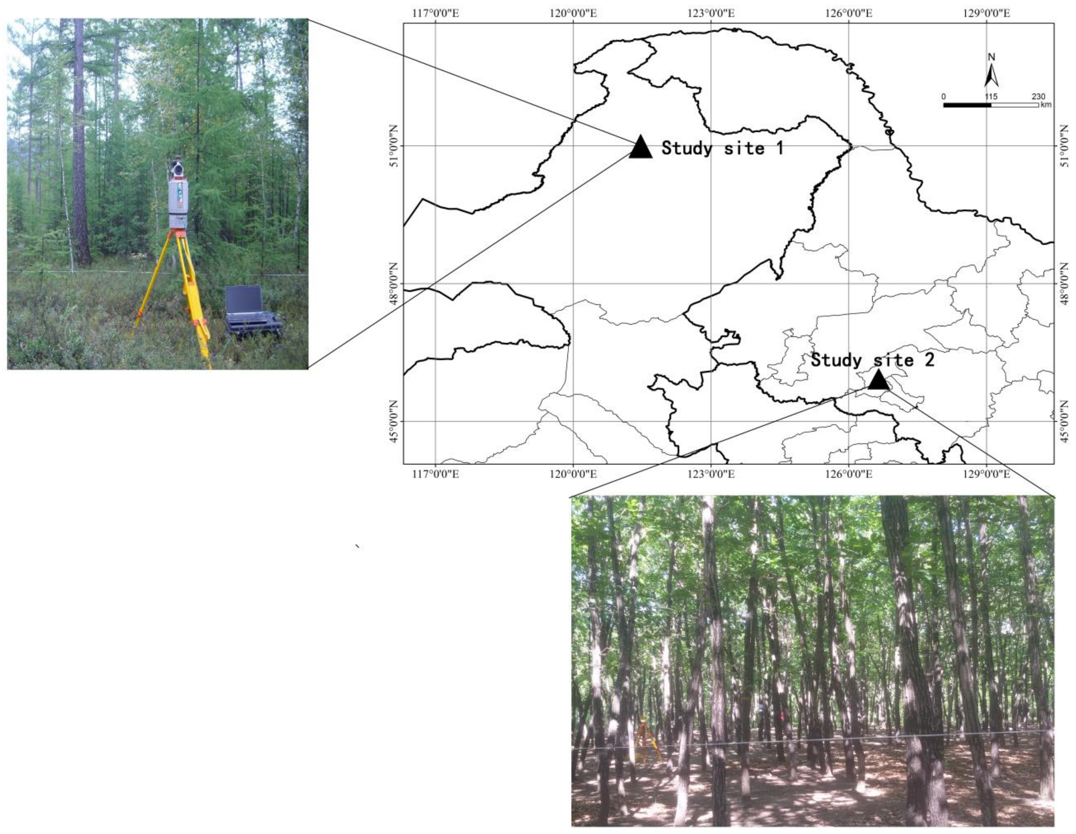
The study area for this study includes two different sites (Figure 1). Site 1 was in a natural forest near the Genhe Ecological Station in HulunBuir city located within Inner Mongolia, China (121°29′35.15″E, 50°56′45.53″N). The forest type was a natural secondary forest. Larch (Larix gmelinii) and white birch (Betula platyphylla) were the dominant tree species in the study site. Larch is valuable for urban planting, and white birch is one of the main tree species found in natural forests in northeast China. The slope of the study site is 12° and the elevation is 874 m. Site 2 was in a Mongolian oak plantation in Harbin city located within Heilongjiang, China (126°37′15.03″E, 45°43′10.66″N). The forest type was a plantation. Mongolian oak (Quercus mongolica) was the dominant tree species in the study site. Mongolian oak is the main tree species in secondary forests in northeast China. The slope of the study site is 5°, and the elevation is 138 m.
2.2. Data
2.2.1. Field Data
Three sample plots were used in the study. Plot 1 and 2 were located in study site 1. Plot 3 was located in study site 2. The plots were 15 m × 15 m squares. Plot 1 trees included 15 larches, seven white birch, and four poplars. The plot shrub height was 0.6 m, and the density was 1156 trees/ha. Plot 2 trees included 14 larches, six white birch, and one poplar. The plot shrub height was 0.78 m, and the density was 933 trees/ha. Plot 3 trees included 54 Mongolian oaks. The plot had little understory vegetation, and the density was 2400 trees/ha. Table 1 shows the descriptive statistics of the tree DBH.
At plot 1 and 2, field measurements (tree position and DBH) were recorded for every tree on the plots on 11 August 2013. At plot 3, field measurements (tree position and DBH) were recorded for every tree on the plot on 1 June 2016. The DBH of each tree was hand-measured by a measuring tape to the nearest millimeter at DBH height (1.3 m vertical above the ground from the base of the tree). The DBH was measured three times for each tree. The arithmetic mean of the three measurements was used for validation of the TLS estimation.
The coordinates of center position of each tree were recorded by a Topcon total station. The accuracy of the total station was 2 mm. The measurement process can be divided into two steps. First the total station measured the position of one point on the stem surface, (xm, ym). Then the position of the stem center (xcenter, ycenter) was calculated according to the position of the measured surface point, filed measured DBH and the positional relationship among total station, the measured surface point and the stem center (Figure 2) via Equations (1) and (2). Note that the z value was also measured by the total station, but it was omitted because it was not needed in the calculation.
2.2.2. Terrestrial Laser Scanning Data
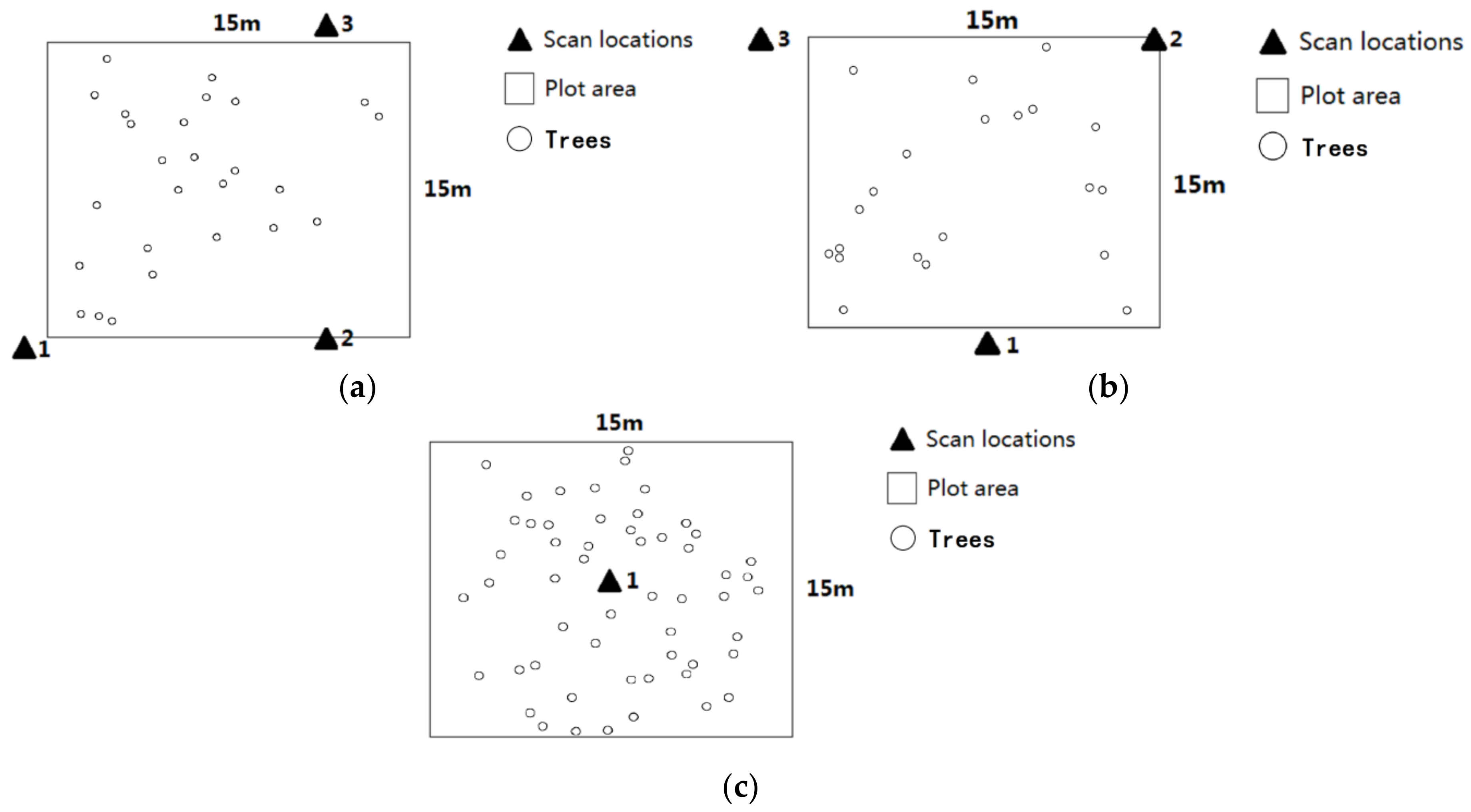
A Riegl Vz-1000 laser scanner and a Trimble GX advanced laser scanner were used in the study. Riegl’s headquarters are located in Horn, Austria. Trimble’s headquarters are located in Sunnyvale, California, USA. At plot 1 and 2, the TLS scans were conducted on 11 August 2013 using the Riegl Vz-1000 laser scanner and a total station. Scanner settings were set to 360° horizontal and 270° vertical field-of-view with an angular resolution of 0.03°. Each plot was scanned with three terrestrial laser scans (Figure 3a,b). Five spherical reference targets were set in the plots. The diameter of the spherical reference target was 145 mm. At plot 3, the TLS scans were conducted on 1 June 2016 using the Trimble GX advanced laser scanner and a total station. Only single scans (360° center scans) were conducted for plot 3 (Figure 3c). Scanner settings were set to 360° horizontal and 140° vertical field-of-view with an angular resolution of 0.03°. Three planar reference targets were set in the plots. For both sites, the positions of the reference targets were measured by TLS and the total station. The coordinates of the reference targets would later be used as the common points in the point cloud co-registration of different scans.
2.3. TLS Data Preprocessing
2.3.1. Co-Registration, TLS Data Thinning, and Elevation Normalization
The raw TLS data was processed through two point-cloud datasets using two different methods. The two datasets were used for further preprocessing and the estimation of DBH. The first dataset consisted of the single-scan TLS data. This implied that only one station’s data was preserved for each plot. Data from station 3 of plot 1, station 2 of plot 2 and station 1 of plot 3 were preserved as point cloud data. This single-scan dataset was named “single-scan mode.” For the second dataset, point cloud data from three scans of plot 1 and 2 were co-registered. The point clouds from different scans were converted to the same coordinate system by using the common points. This dataset was named “multi-scan mode.” Plot 3 did not have multi-scan dataset, since only single scans were conducted at the plot. The dataset of plot 1 and 2 would be analysis together in the further experiment, since they were both located in site 1 and had the same forest type.
Point cloud data that fell out of the plot was removed. The preserved data was thinned to decrease the enormous DBH processing time caused by the numerous preprocessing conditions. The thin-out value depended on the maximum point spacing that did not decrease the accuracy of DBH estimation. This point spacing could be calculated according to the research of Kankare et al. [33]: the RMSE of estimated DBH increases after 30% sampling densities in their study. Therefore, the point spacing of 30% sampling densities was the maximum point spacing that did not decreasing the accuracy of DBH estimation in their study. According to the original point spacing (6.3 mm at 10 m) of their study, the point spacing in 30% sampling densities could be obtained: 21 mm at 10 m (6.3 mm/30%). This was used as the target point spacing of this study.
The original point spacing of this study could be obtained according to the angle resolution used in the study (0.03°): 5.2 mm at 10 m (10,000 mm × tan(0.03°)). Therefore, the original data was thinned to 1/4 of the original size in order to thin-out the point spacing to ~21 mm at 10 m (5.2 mm × 4 = 20.8 mm). The uniform sampling method was used to thin-out the point cloud data, same as in the study of Kankare et al. [33].
In order to measure the height above ground a digital elevation model (DEM) was generated from the point cloud data using the Triangulated Irregular Network (TIN) algorithm. The TIN algorithm created the DTM by the iterative densification of the triangulated irregular network [34]. The z-value of each point was then normalized by subtracting the corresponding height value of the DEM to obtain the vertical distance to the ground.
2.3.2. Extracting Point Cloud of Individual Stems
The point cloud was filtered before the extraction of individual stems. Height thresholds of 0.3 and 3 m were selected to minimize the effects of crown and understory vegetation and preserve the information useful to estimate DBH. All the points with heights less than 0.3 m or greater than 3 m were removed after elevation normalization. The density of the preserved points had influence on the choice of gray scale threshold. The density of these points with an above ground level (AGL) height of 0.3–3 m was 3322/m3 in plot 1 and 2, and 1230/m3 in plot 3.
The point cloud of the individual stems was extracted from the AGL 0.3–3 m points after filtration. The individual stems were extracted using vertical cut cuboids. The center coordinate of each cuboid was the coordinate of each tree’s position, which was derived from the tree positions recorded by the total station. The distance between trees was irregular. Some small trees were closely grouped, with a minimum distance of only 17 cm (Figure 4). In order to avoid interference from the point clouds of nearby trees, the length of each stem cutting’s cuboid was set to be twice the filed measured DBH of that tree.
2.3.3. Selecting Points for DBH Estimation and Calculating the Projection Binary Images
The approach used to select and process points for DBH estimation is based upon a vertical slicing and 2D projection method. Slice thickness of the point cloud was defined as the “height bin,” the threshold used in the gray scale images as the “gray scale threshold,” and the number of points projected in the grid as the “gray scale value.” The height bin, gray scale threshold, and gray scale values were referred to as H, G and N, respectively.
Each stem’s points with an AGL height of 1.3 m ± H/2 were extracted. These 3D points were projected onto the XOY plane to form a 2D gray scale image. Each grid of the image represented a horizontal area of 5 × 5 mm in the point cloud. The gray scale value of each grid was the number of points projected in the grid. The gray scale images were then converted to binary images according to the gray scale value N: if a grid’s N < G, its value was set to zero; otherwise, the value was set to one. As an example, the sliced binary images of five stems of plot 1 and 2 at one preprocessing condition in multi-scan mode are shown in Figure 5. The binary images of these five stems in single-scan mode are shown in Figure 6. And the binary images of five stems of plot 3 are shown in Figure 7.
Signal-Noise Radio (SNR) (the number of stem points/the number of non-stem points) was introduced to evaluate the quality of the images. The binary images of plot 1 and 2 had low SNR due to large numbers of outlier points and the invisibility of stems, especially in single-scan mode. The SNR of binary images in plot 3 was high due to the few numbers of outlier points.
Numerous preprocessing conditions (different H and G values) were used in the study. The range of H and G in different plots and scan modes is summarized in Table 2. There was a total of 104 preprocessing conditions in multi-scan mode of plot 1 and 2, 262 preprocessing conditions in single scan mode of plot 1 and 2, and 420 preprocessing conditions in plot 3.
2.4. Algorithms Used in DBH Estimation
Three commonly used DBH estimation algorithms were evaluated: the Hough-Transform [35], a linear least square algorithm (Landau algorithm) [36] implemented by Sumith [37], and a nonlinear least square algorithm implemented by Brown [38].
The Hough-Transform transforms given points from the image space into accumulator votes in the parameter space, or the Hough space. In the image space, Equation (3) describes a circle with center (a, b) and radius r.
If (x, y) is considered as a foreground pixel of the image, the parameters (a, b, r) in 3D transform space can be found via Equation (3). An accumulative matrix, based on votes in the transform space, is constructed and local maximums will be considered as parameters of circles in the image [35]. A major concern using the Hough-Transform is that the density distribution of the point in the image will have a large influence on the algorithm.
The Landau circle fitting algorithm is a linear least square algorithm. It uses a non-iterative fit which makes it computationally efficient [36].
The nonlinear least square algorithm is a standard approach to fitting circles to a 2D image. It minimizes the function as Equation (4),
where (a, b) denotes the center of the circle and R denotes the radius; di stands for the distance from (xi, yi) to the circle [39], as shown in Equations (5) and (6). The algorithm returns the maximum likelihood estimates (MLE) of the circle parameters [39]. A major concern when using the nonlinear least square algorithm is that the respective minimization algorithms have no closed solution, and therefore they require iterative and computationally intensive numeric schemes such as a general Gauss-Newton or Levenberg-Marquardt [19]. These schemes may converge to a local minimum rather than the global minimum. Therefore, the robustness of the algorithm is relatively poor. Gauss-Newton was used in the nonlinear least square algorithm in this study.
2.5. Estimation of DBH
After the preprocessing procedures, the DBH estimation algorithms described in Section 2.4 were applied to the binary image of each stem. The DBH was then estimated as the diameter of the fitted circle of the algorithms.
2.6. Accuracy Evaluation
The TLS estimations were compared with the field measurements. The accuracy of the estimated DBH at the tree level was evaluated by calculating R2, RMSE, relative RMSE, and relative accuracy (Equations (7) and (8)). The relative RMSE and the relative accuracy were calculated according to the mean value of field measured DBH.
When the height bin and gray scale threshold were not appropriate, some algorithms might produce a large deviation due to the invisibility of stems, or the presence of many outlier points in the image. To avoid affecting the accuracy of the analysis, the result was preserved only if the relative accuracy was between zero and one. The relative accuracy value of the rest of the results was set to zero.
3. Results and Discussion
3.1. Dataset of Multi-Scan Mode
The performance of the Hough-Transform was worse than the other two algorithms in multi-scan mode of the natural secondary forest, producing a maximum relative accuracy lower than 0.14 (Figure 8). Physically, plots were located in a natural forest with heavy understory and branches, which resulted in enormous numbers of outlier points and a relatively low SNR of the binary images. Hough-Transform was based on the accumulative matrix in the transform space, so many outlier points in the image would significantly influence the accuracy. Hough-Transform was not appropriate in the natural forest with heavy understory vegetation and branches in multi-scan mode.
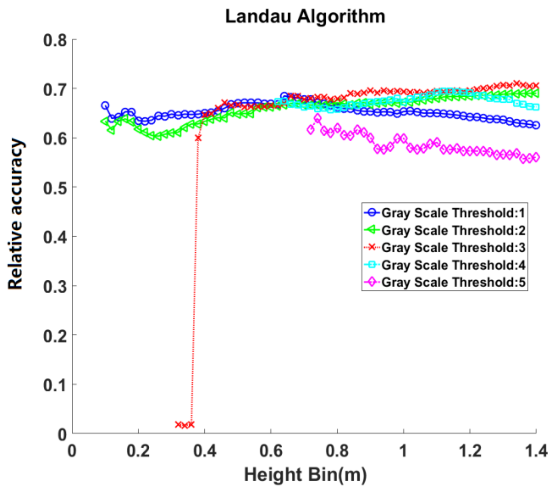
In multi-scan mode, the Landau algorithm achieved its highest accuracy with a height bin of 0.1 m and a gray scale threshold of three with a R2 of 0.97, a RMSE of 1.77 cm and a relative RMSE of 12.2%. The overall accuracy of the Landau algorithm showed a declining trend as the height bin increased. Only at a gray scale threshold of four, accuracy showed an increasing trend up to the maximum accuracy point (with a height bin of 0.16 m, relative accuracy of 0.87) and then a declining trend (Figure 9). Although only three scanning stations were conducted in the plots, there was high stem visibility in multi-scan mode. Therefore, a small height bin (0.1–0.24 m) was able to encompass enough stem circumference information. In this context, the projection binary images contained more outlier points as the height bin increased, and the effect of circle fitting inclined stem point clouds was also increased, causing a decrease in the accuracy of DBH retrieval.
For the gray scale threshold, estimation accuracy was greatest at the gray scale threshold of three in most height bins, with decreased accuracy at thresholds of two and four, and the least accuracy at one. Due to heavy understory vegetation and branches, it was difficult to remove outlier points with a small gray scale threshold. As the stem circumference information would be incomplete if a large threshold was used, a moderate threshold of three had the best performance (Figure 9).
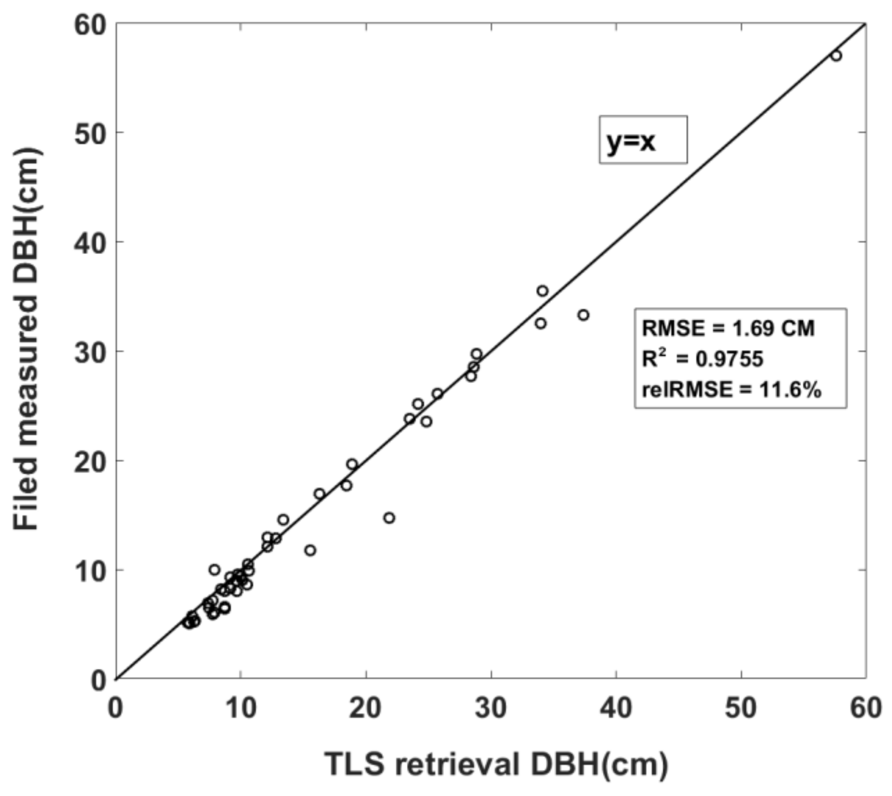
In multi-scan mode, the nonlinear least square algorithm was most accurate at the height bin of 0.24 m with a gray scale threshold of 3. The R2 was 0.98, the RMSE was 1.69 cm, and the relative RMSE was 11.6%. The accuracy trend of the nonlinear least square algorithm along with the height bin and gray scale threshold was similar to that of the Landau algorithm. The algorithm had greater accuracy when the gray scale threshold ranged from 2–4, and the height bin was 0.1–0.24 m (Figure 10). This height bin increased as the threshold increased. This implied that a larger height bin was needed to contain more stem information as the threshold increased.
In multi-scan mode of the natural secondary forest, the nonlinear least square algorithm obtained the most accurate results of all the tested algorithms. Figure 11 shows the scatter plot of TLS estimated DBH versus field measured DBH in the multi-scan mode of the natural secondary forest, which provided the most accuracy (nonlinear least square algorithm, a height bin of 0.24 m, and a gray scale threshold of 3).
The Landau and nonlinear least square algorithms were more accurate under the preprocessing condition of a small height bin (0.1–0.24 m) and a moderate gray scale threshold (both three). The stems could be scanned from multiple directions in the multi-scan mode, which meant the stems were complete in the point cloud data. A small height bin could contain complete stem circumference information. A moderate gray scale threshold is needed to overcome the outlier points caused by the presence of branches and shrubs. When compared with the potential issue resulting from limited visibility of stems in a natural forest, the presence of outlier points was the main cause of DBH estimation bias when using multi-scan mode in the natural secondary forest. Multi-scan methods improved the potential problem of low stem visibility, while the outlier points caused by the presence of branches and shrubs impacted DBH estimation from TLS data.
In most previous 2D-slice studies, DBH was estimated from a fixed small height bin of approximately 0.1 m [19,20,26]. This study showed that a height bin range of 0.1–0.24 m and a moderate threshold of three were more appropriate for multi-scan mode of the natural secondary forest. Using these parameters, the projection binary images had a better SNR and were able to contain more stem circumference information with fewer outlier points. The Landau algorithm had the best overall performance than the other algorithms. Although the best accuracy of Landau algorithm was slightly worse (R2 = 0.97 vs. 0.98 and RMSE 1.69 cm vs. 1.77 cm) than the nonlinear least square algorithm, the Landau algorithm was simpler and less depending on the preprocessing conditions (Figure 9). In a natural forest, combining this algorithm and preprocessing condition could provide a high accuracy DBH estimation result that could be automatically obtained from a TLS point cloud using multi-scan mode.
3.2. Dataset of Single-Scan Mode
Similar to its performance in multi-scan mode, the Hough-Transform had the least successful single-scan mode results in the natural secondary forest. The maximum relative accuracy of the Hough-Transform was lower than 0.12 (Figure 12) for the same reasons as in multi-scan mode of the natural secondary forest.
The performance of the Hough-Transform in plot 3 was better than plot 1 and 2. The maximum relative accuracy was 0.76 (with a height bin of 0.08 m and a gray scale threshold of two). The overall accuracy of the Hough-Transform showed an increasing and then a declining trend as the height bin increased (Figure 13). The height bin started from a small value in plot 3, 0.02 m. The stem circumference was incomplete in the binary images due to the small height bin. The binary images could contain more stem circumference information as the height bin increased. Therefore, the overall accuracy of DBH estimation increased as the height bin increased in the range of 0.02–0.2 m. The height bin of the maximum accuracy point for each gray scale threshold increased as the gray scale threshold increased. This implied that a larger height bin was needed to contain enough stem information as the threshold increased.
Plot 3 was located in a plantation with few understory vegetation. Although only one scanning stations were conducted in the plot, there was relatively high stem visibility due to the sparse understory. Therefore, the height bin of ~0.2 m was enough to contain complete stem circumference information. After the height bin of ~0.2 m, the projection binary images contained more outlier points as the height bin increased, and the effect of circle fitting inclined stem point clouds was also increased, causing a decrease in the accuracy of DBH retrieval.
For gray scale threshold, the overall estimation accuracy decreased as the gray scale threshold increased. Due to sparse understory and branches, there were few numbers of outlier points in the binary images. The gray scale threshold was not needed to overcome the outlier points. Instead, more stem points would be removed as the gray scale threshold increased, causing the incomplete of stem circumference and a decrease in the accuracy of DBH estimation.
The nonlinear least square algorithm was less accurate in single-scan mode of the natural secondary forest. The maximum relative accuracy was 0.59 (with a height bin of 0.58 m and a gray scale threshold of one). Compared with multi-scan mode, there were some “zero points,” meaning that the relative accuracy was not within the range of zero to one (Figure 14). These “zero points” resulted from the low SNR of the binary images. The visibility of trees was low in single-scan mode of the natural secondary forest, resulting in incomplete stem circumference information and a low SNR (Figure 6). The nonlinear least square algorithm may converge to the local minimum instead of global minimum, leading to a large bias of the estimated DBH. This implies that the nonlinear least square algorithm had a high input image quality requirement. The algorithm was less stable with low accuracy when the image quality was low. Therefore, the nonlinear least squares algorithm is not an appropriate choice for single-scan mode of the natural secondary forest.
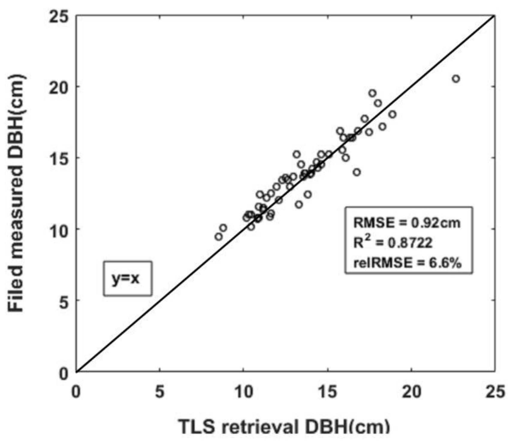
The maximum accuracy of the nonlinear least square algorithm in plot 3 was obtained under the height bin of 0.1 m and the gray scale threshold of 1: R2 0.87, RMSE 0.92 cm, and relative RMSE 6.63%. At the gray scale threshold of 1–3, the accuracy of the nonlinear least square algorithm showed an increasing and then a declining trend as the height bin increased (Figure 15). The height bin of the maximum accuracy point for each gray scale threshold was 0.1, 0.1, and 0.22 m, respectively. Like described in the Hough-Transform of plot 3, the stem circumference was incomplete under the small height bin; while the projection binary images contained more outlier points and the effect of circle fitting inclined stem point clouds was also increased under the large height bin. Therefore, a moderate height bin of 0.1–0.22 m was the most optimal parameterization.
The algorithm was not stable at thresholds of 4–7, and some “zero points” appeared. The accuracy of the algorithm decreased to zero for all the gray scale thresholds after the height bin increased to 0.56 m. More stem points would be removed under the large gray scale threshold, causing the incomplete of stem circumference and a low quality of the binary images. Similarly, more outlier points were preserved and the effect of circle fitting inclined stem point clouds increased due to the excessive height bin, causing the low SNR of the binary images. The algorithm was not able to obtain accurate results from the low SNR images, as described in the single-scan mode of the natural secondary forest. The accuracy decreased to zero. The results showed that the nonlinear least square algorithm had a high requirement on input image quality, a moderate small height bin (0.1–0.22 m) and a small gray scale threshold (1–3) were appropriate when using this algorithm in the plantation.
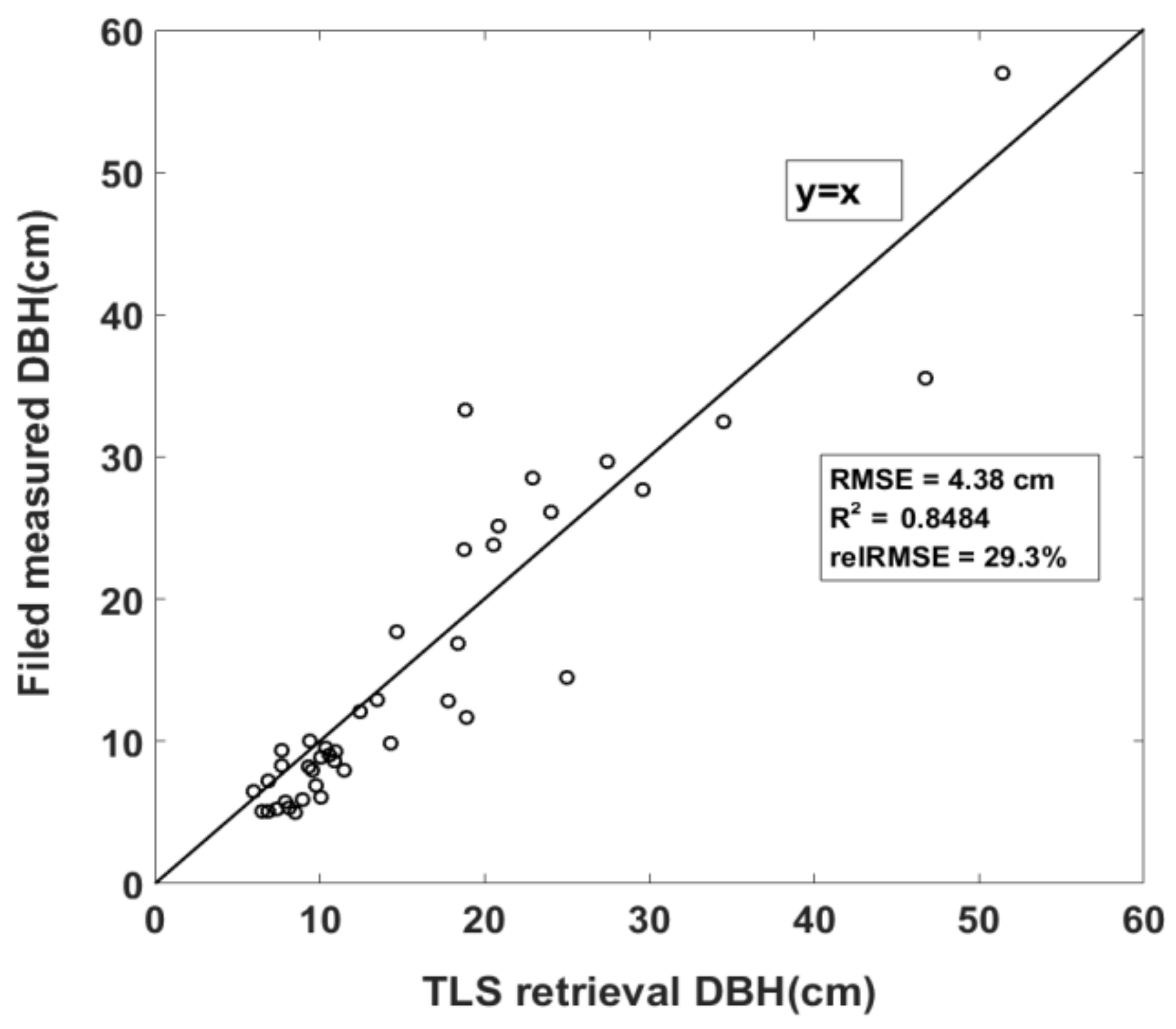
In single scan mode of the natural secondary forest, the maximum accuracy of the Landau algorithm was obtained under the height bin of 1.34 m and the gray scale threshold of 3: R2 0.85, RMSE 4.38 cm and relative RMSE 29.3%. At the gray scale threshold of one and four, the accuracy of the Landau algorithm showed an increasing and then a declining trend (Figure 16). The accuracy increased at thresholds of two and three and decreased at a threshold of five as the height bin increased. The Landau algorithm was more accurate when the gray scale threshold ranged from two to four, and the height bin was 1.2–1.4 m. The highest accuracy was reached using a gray scale threshold of three. In previous studies [19,20,26,27,29], slices corresponding to a large height bin, such as 1.34 m, had not been used.
The projection binary images had a lower SNR because of the low visibility of the trees in single-scan mode of the natural secondary forest (Figure 6). When the height bin was relatively large, the projection binary images could contain more stem circumference information. Therefore, the Landau algorithm was able to perform well. At the same time, the projection binary images also contained more outlier points due to the larger height bin, decreasing the overall accuracy of the Landau algorithm. To ensure that there is sufficient capacity to remove the outlier points, the gray-scale threshold should be relatively large.
In plot 3, the Landau algorithm was most accurate under the height bin of 0.02 m with a gray scale threshold of 1. The R2 was 0.64, the RMSE was 1.55 cm, and the relative RMSE was 11.2%. The accuracy decreased slightly as the height bin increased (Figure 17). The reason why the accuracy decreased was similar to that of the Hough-Transform in plot 3. The algorithm had lower accuracy under a small height bin and a large gray scale threshold (5–7). The projection binary images had less stem points under a small height bin, meanwhile a large gray scale threshold removed more stem points, causing an incomplete of the stem circumference information. Therefore, the accuracy of the algorithm was low due to the lack of the stem circumference.
For gray scale threshold, the accuracy decreased as the gray scale threshold increased. The reason was similar to that of the Hough-Transform in plot 3. The accuracy of Landau algorithm had less variation under different preprocessing conditions. This implied that Landau algorithm was less depending on the chosen preprocessing conditions and therefore more robust than the other two algorithms.
The Landau algorithm showed maximum accuracy of all algorithms tested in single-scan mode of the natural secondary forest. Figure 18 shows the scatter plot of TLS estimated DBH and field measured DBH using the most accurate single-scan mode method in the natural secondary forest (Landau algorithm, a height bin of 1.34 m, and a gray scale threshold of 3).
The nonlinear least square algorithm obtained the most accurate results of all the tested algorithms in plot 3. Figure 19 shows the scatter plot of TLS estimated DBH versus field measured DBH in the plantation, which provided the most accuracy (nonlinear least square algorithm, a height bin of 0.1 m, and a gray scale threshold of 1).
Compared with the results of multi-scan mode, the accuracy of the nonlinear least square algorithm was greatly influenced by the image quality. The accuracy was low and unstable when the tree circumference was incomplete, and the SNR of the slice image was low. The results showed that it was less robust than the Landau algorithm. This was due to the algorithm possibly converging to a local minimum rather than the global minimum, as described in Section 2.4. However, compared with the results of plot 1 and 2, the nonlinear least square algorithm had a high accuracy due to the high SNR of the slice images in plot 3 (Figure 7). The results showed that the nonlinear least square algorithm had the best performance among the three tested algorithms when the quality of the images was high.
In all the plots, the Landau algorithm was less depending on the preprocessing conditions and the quality of the images. The algorithm was more robust (the “zero point” rarely appeared) and had a higher accuracy for single-scan mode of the natural secondary forest with lower SNR. This implied that the Landau algorithm was most robust and stable among the three tested algorithms. However, the Landau algorithm’s accuracy was not as good as the nonlinear least square algorithm when the image quality was high. The performance of Hough-Transform was worse than the other two algorithms in all the plots. Overall, the nonlinear least square algorithm was preferable for the plantation with a higher quality of projection binary images. The Landau algorithm was preferable for the natural secondary forest with enormous numbers of outlier points and a lower SNR.
The accuracies of algorithms in plot 3 were higher (Table 3) and also had less variation compared with the results in plot 1 and 2. The differences of the forest condition between the plots may be the main cause. Plot 1 and 2 was inside a natural secondary forest. The forest condition was complex featuring dense understory vegetation and tree branches. This forest condition resulted in enormous numbers of outlier points and a relatively low SNR of the binary images, as shown in Figure 5 and Figure 6. The algorithms may produce a large bias under some preprocessing conditions due to the low quality of the images. This would result in the worse accuracy and the high variations of the results. The forest condition of plot 3 was simple, featuring little understory vegetation and few tree branches. This resulted in fewer outlier points in the binary images (Figure 7). The algorithms were more stable and accurate due to the high quality of the images, even though only the single-scan scanning method was conducted.
This study focused on evaluating different methods for extracting DBH and did not incorporate automatic stem delineation algorithms in order to ensure that all stems are identified. For an operational application, there were various methods of automatic stem mapping from TLS data [40]. Our results can be easily combined with these automatic stem mapping methods to retrieve stem position and DBH rapidly with low time and labor cost.
4. Conclusions
This study evaluated three commonly used DBH estimation algorithms (the Hough-transform, linear least square circle fitting, and nonlinear least square circle fitting) on their performance using two forest types of TLS data under numerous preprocessing conditions. The two forest types were natural secondary forest and plantation. The following conclusions can be drawn from this study:
- The linear least square circle fitting algorithm was more appropriate for the natural secondary forest than the other algorithms. The nonlinear least square circle fitting algorithm was preferable for the plantation. The performance of the Hough-Transform was poor.
- A moderate gray scale threshold of three was the most optimal parameterization for the natural secondary forest. A small gray scale threshold of one was the most optimal parameterization for the plantation.
- In the natural secondary forest, a moderately large height bin of 0.24 m was appropriate for the multi-scan scanning method, and a large height bin of 1.34 m was appropriate for the single-scan scanning method. A small height bin of 0.1 m was appropriate for the single-scan scanning method in the plantation.
This study provides guidance for choosing the most appropriate algorithm and preprocessing condition to estimate DBH from TLS data. While these results were obtained in a natural secondary forest and a plantation, the applications of the results in other forest conditions need to be validated in future studies.
Acknowledgments
This work is supported by the Special Fund for Forest Scientific Research in the Public Welfare (No. 201504319), the National Key R&D Program of China (Granted: 2017YFD0600904), and the National Basic Research Program of China (Granted: 2013CB733404).
Author Contributions
Chang Liu conceived and designed the experiments, performed the experiments, analyzed the data and wrote the paper. Yanqiu Xing and Xin Tian assisted with data collection. Yanqiu Xing secured funding for the project, provided valuable suggestions for the overall design of the study, and reviewed the manuscript. Jialong Duanmu polished the language of the manuscript.
Conflicts of Interest
The authors declare no conflict of interest. The founding sponsors had no role in the design of the study; in the collection, analyses, or interpretation of data; in the writing of the manuscript, and in the decision to publish the results.
References
- Liang, X.; Kankare, V.; Hyyppä, J.; Wang, Y.; Kukko, A.; Haggrén, H.; Yu, X.; Kaartinen, H.; Jaakkola, A.; Guan, F.; et al. Terrestrial laser scanning in forest inventories. ISPRS J. Photogramm. Remote Sens. 2016, 115, 63–77. [Google Scholar] [CrossRef]
- Aschoff, T.; Thies, M.; Spiecker, H. Describing forest stands using terrestrial laser-scanning. Int. Arch. Photogramm. Remote Sens. Spat. Inf. Sci. 2004, 35, 237–241. [Google Scholar]
- Hopkinson, C.; Chasmer, L.; Youngpow, C.; Treitz, P. Assessing forest metrics with a ground-based scanning lidar. Can. J. For. Res. 2004, 34, 573–583. [Google Scholar] [CrossRef]
- Watt, P.J. Measuring forest structure with terrestrial laser scanning. Int. J. Remote Sens. 2005, 26, 1437–1446. [Google Scholar] [CrossRef]
- Henning, J.G.; Radtke, P.J. Detailed stem measurements of standing trees from ground-based scanning lidar. For. Sci. 2006, 52, 67–80. [Google Scholar]
- Maas, H.G.; Bienert, A.; Scheller, S.; Keane, E. Automatic forest inventory parameter determination from terrestrial laser scanner data. Int. J. Remote Sens. 2008, 29, 1579–1593. [Google Scholar] [CrossRef]
- Huang, H.; Li, Z.; Gong, P.; Cheng, X.; Clinton, N.; Cao, C.; Ni, W.; Wang, L. Automated methods for measuring dbh and tree heights with a commercial scanning lidar. Photogramm. Eng. Remote Sens. 2011, 77, 219–227. [Google Scholar] [CrossRef]
- Vonderach, C.; Vögtle, T.; Adler, P.; Norra, S. Terrestrial laser scanning for estimating urban tree volume and carbon content. Int. J. Remote Sens. 2012, 33, 6652–6667. [Google Scholar] [CrossRef]
- Pueschel, P. The influence of scanner parameters on the extraction of tree metrics from faro photon 120 terrestrial laser scans. ISPRS J. Photogramm. Remote Sens. 2013, 78, 58–68. [Google Scholar] [CrossRef]
- Liang, X.; Kankare, V.; Yu, X.; Hyyppa, J.; Holopainen, M. Automated stem curve measurement using terrestrial laser scanning. IEEE Trans. Geosci. Remote Sens. 2014, 52, 1739–1748. [Google Scholar] [CrossRef]
- Bauwens, S.; Bartholomeus, H.; Calders, K.; Lejeune, P. Forest inventory with terrestrial lidar: A comparison of static and hand-held mobile laser scanning. Forests 2016, 7, 127. [Google Scholar] [CrossRef]
- You, L.; Tang, S.; Song, X.; Lei, Y.; Zang, H.; Lou, M.; Zhuang, C. Precise measurement of stem diameter by simulating the path of diameter tape from terrestrial laser scanning data. Remote Sens. 2016, 8, 717. [Google Scholar] [CrossRef]
- Saarinen, N.; Kankare, V.; Vastaranta, M.; Luoma, V.; Pyörälä, J.; Tanhuanpää, T.; Liang, X.; Kaartinen, H.; Kukko, A.; Jaakkola, A.; et al. Feasibility of terrestrial laser scanning for collecting stem volume information from single trees. ISPRS J. Photogramm. Remote Sens. 2017, 123, 140–158. [Google Scholar] [CrossRef]
- Wang, D.; Kankare, V.; Puttonen, E.; Hollaus, M.; Pfeifer, N. Reconstructing stem cross section shapes from terrestrial laser scanning. IEEE Geosci. Remote Sens. Lett. 2017, 14, 272–276. [Google Scholar] [CrossRef]
- Tansey, K.; Selmes, N.; Anstee, A.; Tate, N.J.; Denniss, A.; Mcroberts, R.E.; Donoghue, D.N.M.; Deshayes, M. Estimating tree and stand variables in a corsican pine woodland from terrestrial laser scanner data. Int. J. Remote Sens. 2009, 30, 5195–5209. [Google Scholar] [CrossRef]
- Trochta, J.; Krucek, M.; Vrska, T.; Kral, K. 3d forest: An application for descriptions of three-dimensional forest structures using terrestrial lidar. PLoS ONE 2017, 12, e0176871. [Google Scholar] [CrossRef] [PubMed]
- Heinzel, J.; Huber, M.O. Tree stem diameter estimation from volumetric tls image data. Remote Sens. 2017, 9, 614. [Google Scholar] [CrossRef]
- Simonse, M.; Aschoff, T.; Spiecker, H.; Thies, M.; Simonse, M.; Aschoff, T.; Spiecker, H.; Thies, M. Automatic determination of forest inventory parameters using terrestrial laser scanning. Proc. Scandlaser Sci. Workshop Airborne Laser Scanning For. 2003, 2003, 252–258. [Google Scholar]
- Pueschel, P.; Newnham, G.; Rock, G.; Udelhoven, T.; Werner, W.; Hill, J. The influence of scan mode and circle fitting on tree stem detection, stem diameter and volume extraction from terrestrial laser scans. ISPRS J. Photogramm. Remote Sens. 2013, 77, 44–56. [Google Scholar] [CrossRef]
- Calders, K.; Newnham, G.; Burt, A.; Murphy, S.; Raumonen, P.; Herold, M.; Culvenor, D.; Avitabile, V.; Disney, M.; Armston, J.; et al. Nondestructive estimates of above-ground biomass using terrestrial laser scanning. Methods Ecol. Evol. 2015, 6, 198–208. [Google Scholar] [CrossRef]
- Xi, Z.; Hopkinson, C.; Chasmer, L. Automating plot-level stem analysis from terrestrial laser scanning. Forests 2016, 7, 252. [Google Scholar] [CrossRef]
- Kankare, V.; Liang, X.; Vastaranta, M.; Yu, X.; Holopainen, M.; Hyyppä, J. Diameter distribution estimation with laser scanning based multisource single tree inventory. ISPRS J. Photogramm. Remote Sens. 2015, 108, 161–171. [Google Scholar] [CrossRef]
- Raumonen, P.; Kaasalainen, M.; Åkerblom, M.; Kaasalainen, S.; Kaartinen, H.; Vastaranta, M.; Holopainen, M.; Disney, M.; Lewis, P. Fast automatic precision tree models from terrestrial laser scanner data. Remote Sens. 2013, 5, 491–520. [Google Scholar] [CrossRef]
- Olofsson, K.; Holmgren, J. Single tree stem profile detection using terrestrial laser scanner data, flatness saliency features and curvature properties. Forests 2016, 7, 207. [Google Scholar] [CrossRef]
- Wang, D.; Hollaus, M.; Puttonen, E.; Pfeifer, N. Automatic and self-adaptive stem reconstruction in landslide-affected forests. Remote Sens. 2016, 8, 974. [Google Scholar] [CrossRef]
- Olofsson, K.; Holmgren, J.; Olsson, H. Tree stem and height measurements using terrestrial laser scanning and the ransac algorithm. Remote Sens. 2014, 6, 4323–4344. [Google Scholar] [CrossRef]
- Sun, H.; Wang, G.; Lin, H.; Li, J.; Zhang, H.; Ju, H. Retrieval and accuracy assessment of tree and stand parameters for chinese fir plantation using terrestrial laser scanning. IEEE Geosci. Remote Sens. Lett. 2015, 12, 1993–1997. [Google Scholar] [CrossRef]
- Srinivasan, S.; Popescu, S.; Eriksson, M.; Sheridan, R.; Ku, N.-W. Terrestrial laser scanning as an effective tool to retrieve tree level height, crown width, and stem diameter. Remote Sens. 2015, 7, 1877–1896. [Google Scholar] [CrossRef]
- Wang, D.; Hollaus, M.; Puttonen, E.; Pfeifer, N. Fast and robust stem reconstruction in complex environments using terrestrial laser scanning. ISPRS—Int. Arch. Photogramm. Remote Sens. Spat. Inf. Sci. 2016, XLI-B3, 411–417. [Google Scholar] [CrossRef]
- Wang, D.; Hollaus, M.; Schmaltz, E.; Wieser, M.; Reifeltshammer, D.; Pfeifer, N. Tree stem shapes derived from tls data as an indicator for shallow landslides. Procedia Earth Planet. Sci. 2016, 16, 185–194. [Google Scholar] [CrossRef]
- Project Benchmarking on Terrestrial Laser Scanning for Forestry Applications. Available online: http://www.eurosdr.net/research/project/project-benchmarking-terrestrial-laser-scanning-forestry-applications (accessed on 4 March 2018).
- Terrestrial Laser Scanning in Forest Inventories: Toward International Benchmarks. Available online: https://www.gim-international.com/content/article/terrestrial-laser-scanning-in-forest-inventories (accessed on 4 March 2018).
- Kankare, V.; Puttonen, E.; Holopainen, M.; Hyyppä, J. The effect of tls point cloud sampling on tree detection and diameter measurement accuracy. Remote Sens. Lett. 2016, 7, 495–502. [Google Scholar] [CrossRef]
- Axelsson, P. Dem generation from laser scanner data using adaptive tin models. Int. Arch. Photogramm. Remote Sens. 2000, 33, 111–118. [Google Scholar]
- Mirzaei, M.; Rafsanjani, H.K. An automatic algorithm for determination of the nanoparticles from tem images using circular hough transform. Micron 2017, 96, 86–95. [Google Scholar] [CrossRef] [PubMed]
- Thomas, S.M.; Chan, Y.-T. A simple approach for the estimation of circular arc center and its radius. Comput. Vis. Graph. Image Process. 1989, 45, 362–370. [Google Scholar] [CrossRef]
- Fast Circle Fitting Using Landau Method, Matlab Central. Available online: http://www.mathworks.com/matlabcentral/fileexchange/44219-fast-circle-fitting-using-landau-method (accessed on 15 March 2017).
- Fitcircle, M. Matlab Central. Available online: http://cn.mathworks.com/matlabcentral/fileexchange/15060-fitcircle-m (accessed on 15 March 2017).
- Al-Sharadqah, A.; Chernov, N. Error analysis for circle fitting algorithms. Electron. J. Stat. 2009, 3, 886–911. [Google Scholar] [CrossRef]
- Liang, X.; Litkey, P.; Hyyppa, J.; Kaartinen, H.; Vastaranta, M.; Holopainen, M. Automatic stem mapping using single-scan terrestrial laser scanning. IEEE Trans. Geosci. Remote Sens. 2012, 50, 661–670. [Google Scholar] [CrossRef]
Figure 1.
Location of the study area.

Figure 2.
Positional relationship among total station, the measured surface point, and the stem center.
Figure 2.
Positional relationship among total station, the measured surface point, and the stem center.
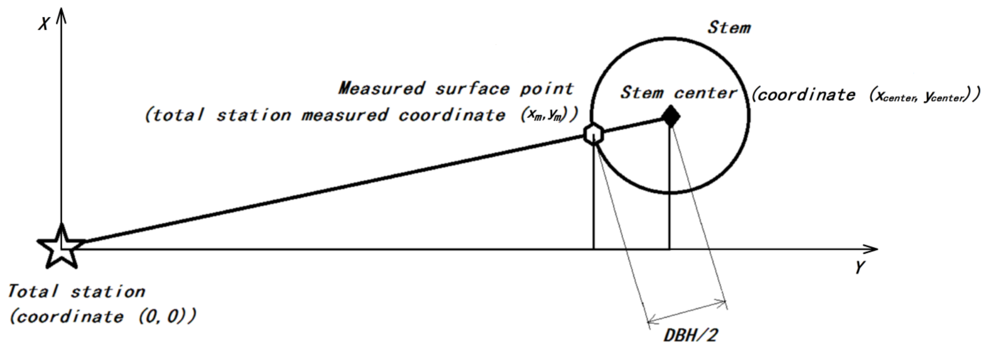
Figure 3.
Scan locations within the plots. (a) plot 1; (b) plot 2; (c) plot 3.

Figure 4.
The most closely grouped trees.

Figure 5.
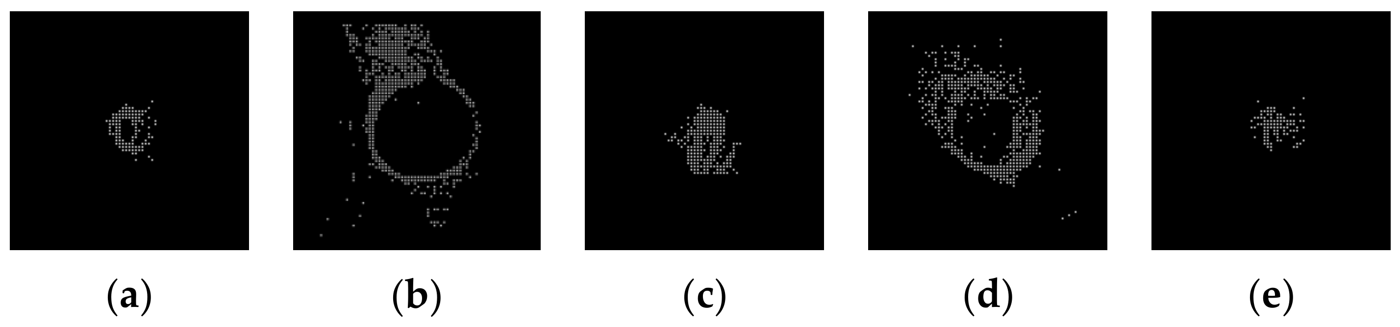
Binary images of five slices of plot 1 and 2 in multi-scan mode with height of 1.25–1.35 m, gray scale threshold of 1. (a) Tree 2; (b) Tree 3; (c) Tree 7; (d) Tree 11; (e) Tree 21.
Figure 5.
Binary images of five slices of plot 1 and 2 in multi-scan mode with height of 1.25–1.35 m, gray scale threshold of 1. (a) Tree 2; (b) Tree 3; (c) Tree 7; (d) Tree 11; (e) Tree 21.

Figure 6.
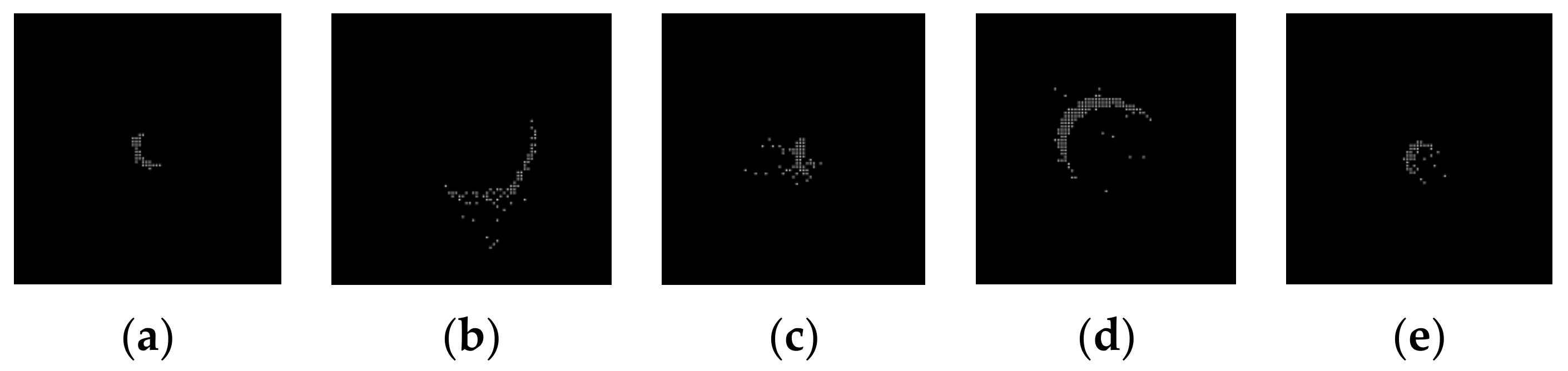
Binary images of five slices of plot 1 and 2 in single-scan mode with height of 1.2–1.35 m, gray scale threshold of 1. (a) Tree 2; (b) Tree 3; (c) Tree 7; (d) Tree 11; (e) Tree 21.
Figure 6.
Binary images of five slices of plot 1 and 2 in single-scan mode with height of 1.2–1.35 m, gray scale threshold of 1. (a) Tree 2; (b) Tree 3; (c) Tree 7; (d) Tree 11; (e) Tree 21.

Figure 7.
Binary images of five slices of plot 3 of single-scan mode with height of 1.25–1.35 m, gray scale threshold of 1. (a) Tree 2; (b) Tree 7; (c) Tree 21; (d) Tree 36; (e) Tree 47.
Figure 7.
Binary images of five slices of plot 3 of single-scan mode with height of 1.25–1.35 m, gray scale threshold of 1. (a) Tree 2; (b) Tree 7; (c) Tree 21; (d) Tree 36; (e) Tree 47.
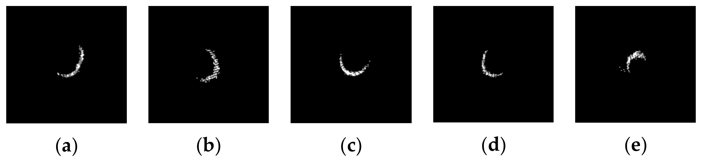
Figure 8.
The relative accuracy of Hough-Transform under different height bins and gray scale thresholds in multi-scan mode of the natural secondary forest.
Figure 8.
The relative accuracy of Hough-Transform under different height bins and gray scale thresholds in multi-scan mode of the natural secondary forest.
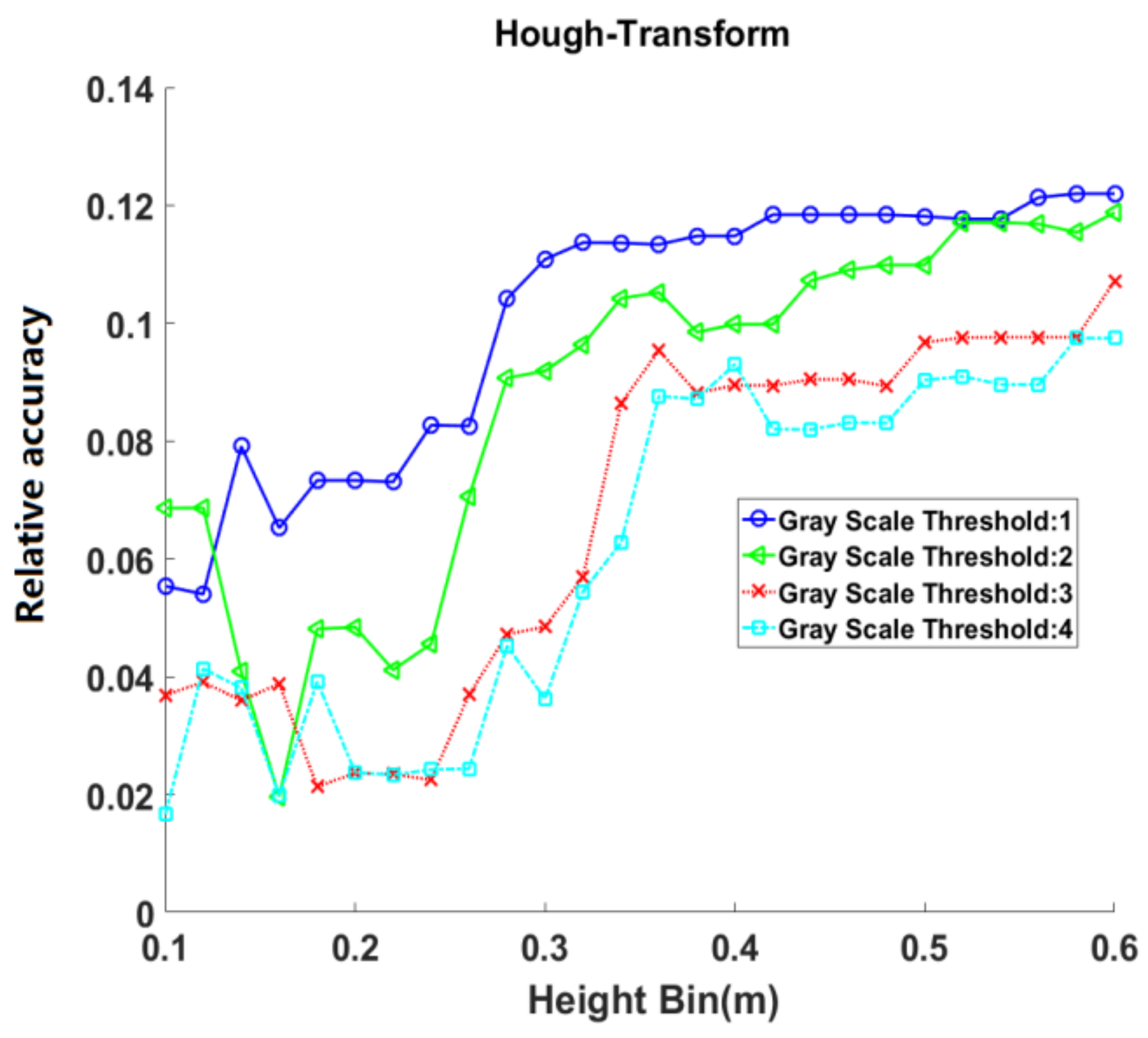
Figure 9.
The relative accuracy of Landau algorithm under different height bins and gray scale thresholds in multi-scan mode of the natural secondary forest.
Figure 9.
The relative accuracy of Landau algorithm under different height bins and gray scale thresholds in multi-scan mode of the natural secondary forest.
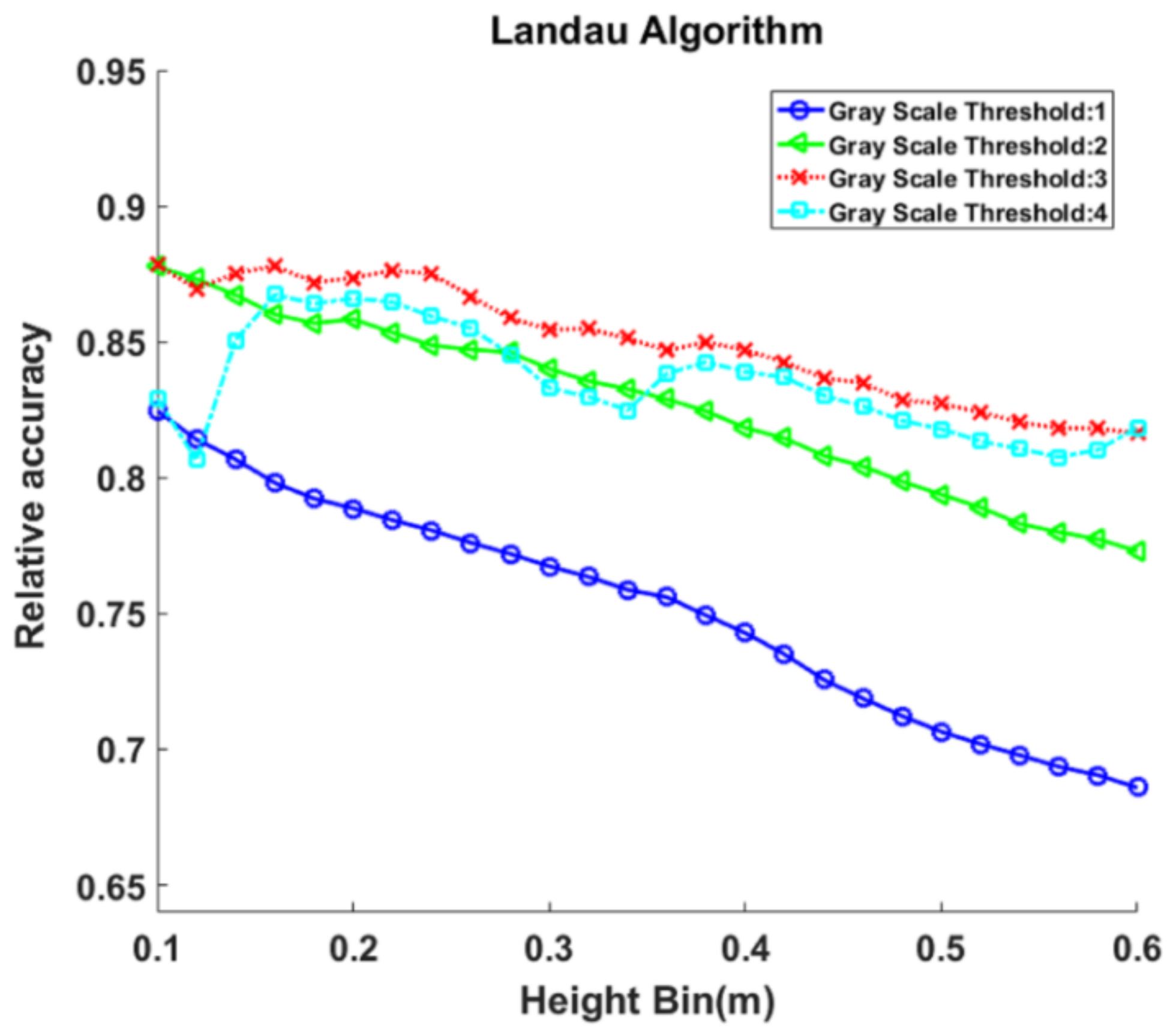
Figure 10.
The relative accuracy of the nonlinear least square circle fitting algorithm (Gauss-Newton) under different height bins and gray scale thresholds in multi-scan mode of the natural secondary forest.
Figure 10.
The relative accuracy of the nonlinear least square circle fitting algorithm (Gauss-Newton) under different height bins and gray scale thresholds in multi-scan mode of the natural secondary forest.
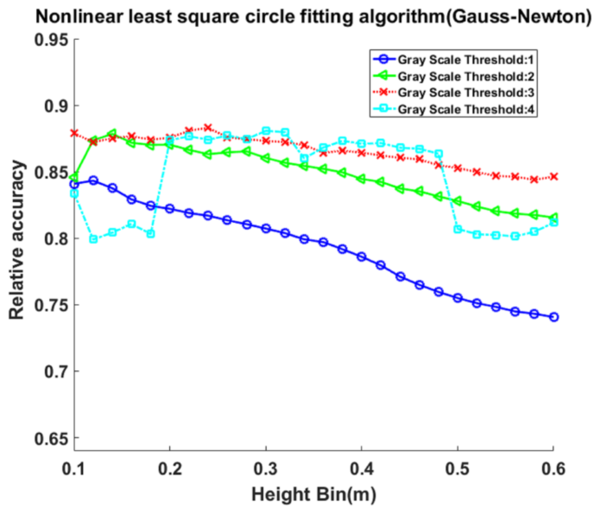
Figure 11.
Scatter plot for terrestrial laser scanning (TLS) estimated versus field measured DBH, in the best accuracy condition of multi-scan mode of the natural secondary forest (nonlinear least square algorithm, a height bin of 0.24 m, and a gray scale threshold of 3).
Figure 11.
Scatter plot for terrestrial laser scanning (TLS) estimated versus field measured DBH, in the best accuracy condition of multi-scan mode of the natural secondary forest (nonlinear least square algorithm, a height bin of 0.24 m, and a gray scale threshold of 3).

Figure 12.
The relative accuracy of Hough-Transform under different height bins and gray scale thresholds in single-scan mode of the natural secondary forest.
Figure 12.
The relative accuracy of Hough-Transform under different height bins and gray scale thresholds in single-scan mode of the natural secondary forest.
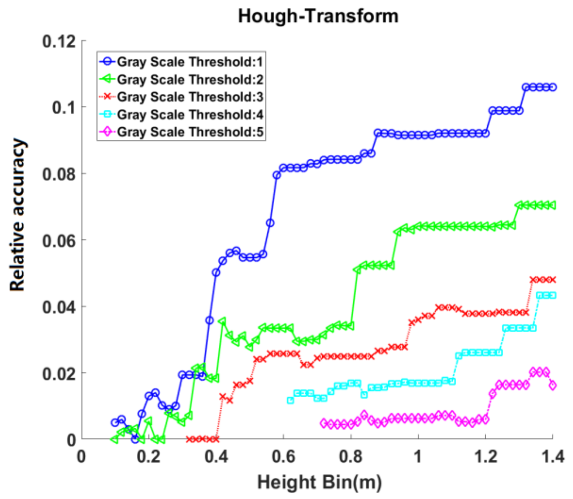
Figure 13.
The relative accuracy of Hough-Transform under different height bins and gray scale thresholds in single-scan mode of the plantation.
Figure 13.
The relative accuracy of Hough-Transform under different height bins and gray scale thresholds in single-scan mode of the plantation.
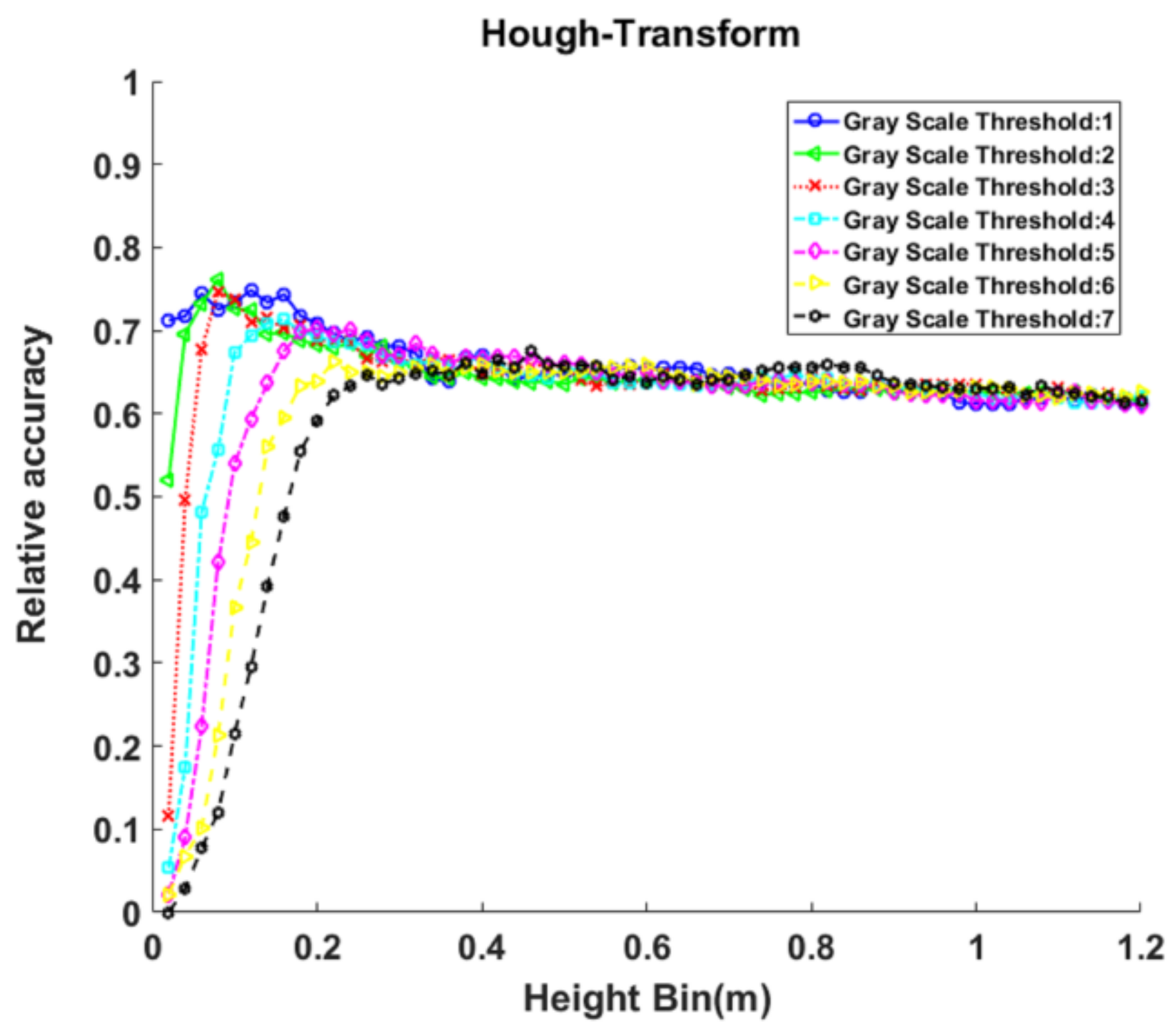
Figure 14.
The relative accuracy of nonlinear least square circle fitting algorithm (Gauss-Newton) under different height bins and gray scale thresholds in single-scan mode of the natural secondary forest.
Figure 14.
The relative accuracy of nonlinear least square circle fitting algorithm (Gauss-Newton) under different height bins and gray scale thresholds in single-scan mode of the natural secondary forest.
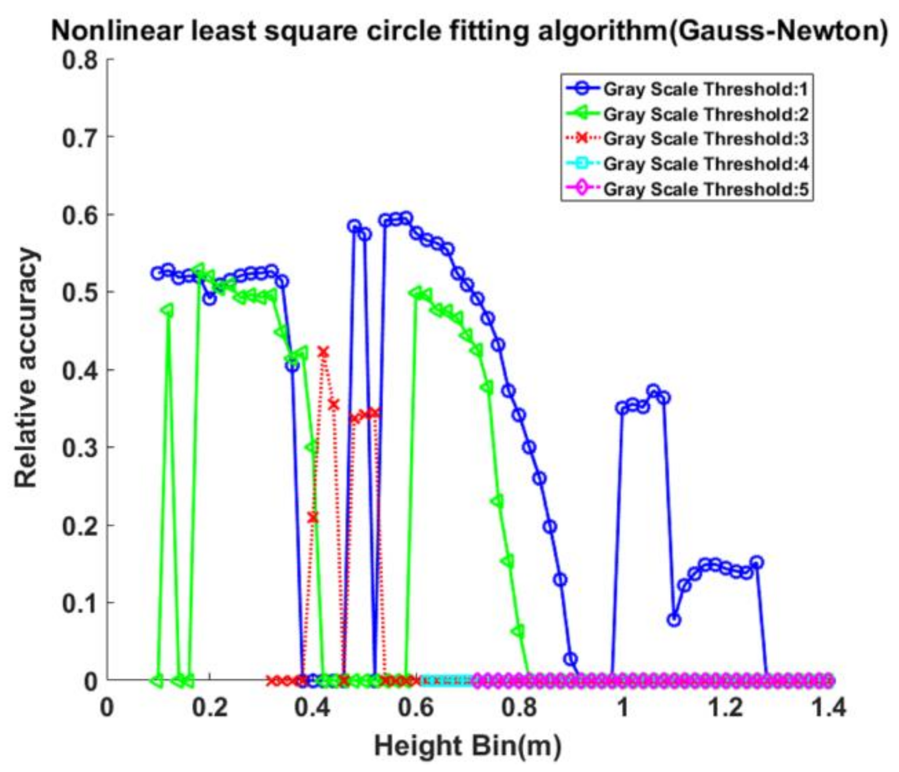
Figure 15.
The relative accuracy of nonlinear least square circle fitting algorithm (Gauss-Newton) under different height bins and gray scale thresholds in single-scan mode of the plantation.
Figure 15.
The relative accuracy of nonlinear least square circle fitting algorithm (Gauss-Newton) under different height bins and gray scale thresholds in single-scan mode of the plantation.

Figure 16.
The relative accuracy of Landau algorithm under different height bins and gray scale thresholds in single-scan mode of the natural secondary forest.
Figure 16.
The relative accuracy of Landau algorithm under different height bins and gray scale thresholds in single-scan mode of the natural secondary forest.

Figure 17.
The relative accuracy of Landau algorithm under different height bins and gray scale thresholds in single-scan mode of the plantation.
Figure 17.
The relative accuracy of Landau algorithm under different height bins and gray scale thresholds in single-scan mode of the plantation.
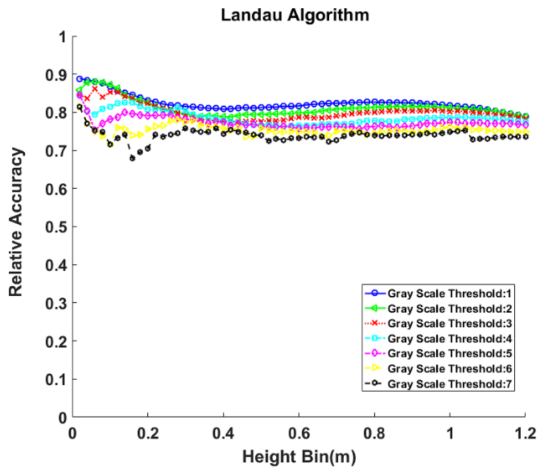
Figure 18.
Scatter plot for TLS estimated versus field measured DBH, in the best accuracy condition of single-scan mode of the natural secondary forest (Landau algorithm, a height bin of 1.34 m, and a gray scale threshold of 3).
Figure 18.
Scatter plot for TLS estimated versus field measured DBH, in the best accuracy condition of single-scan mode of the natural secondary forest (Landau algorithm, a height bin of 1.34 m, and a gray scale threshold of 3).

Figure 19.
Scatter plot for TLS estimated versus field measured DBH, in the best accuracy condition of single-scan mode of the plantation (nonlinear least square algorithm, a height bin of 0.1 m, and a gray scale threshold of 1).
Figure 19.
Scatter plot for TLS estimated versus field measured DBH, in the best accuracy condition of single-scan mode of the plantation (nonlinear least square algorithm, a height bin of 0.1 m, and a gray scale threshold of 1).


Table 1.
Descriptive statistics of the diameter at breast height (DBH) for the test plots by tree species and all together.
Table 1.
Descriptive statistics of the diameter at breast height (DBH) for the test plots by tree species and all together.
| Plot | Species | DBH (cm) | ||
|---|---|---|---|---|
| Min | Max | Mean | ||
| 1 | Larch | 5.1 | 17.7 | 7.8 |
| White birch | 6.4 | 33.3 | 22.2 | |
| Poplar | 10.5 | 23.8 | 18.7 | |
| All | 5.1 | 33.3 | 13.3 | |
| 2 | Larch | 6.6 | 57 | 16.1 |
| White birch | 5 | 27.7 | 14.4 | |
| Poplar | 32.5 | 32.5 | 32.5 | |
| All | 5 | 57 | 16.4 | |
| 3 | Mongolian oak | 9.5 | 20.5 | 13.8 |
Table 2.
Range of height bin and gray scale threshold in different plots and scan modes.
| Plot | Scan Mode | Range of Height Bin (m) 1 | Range of Gray Scale Threshold 2 |
|---|---|---|---|
| 1, 2 | Multi-scan | 0.1–0.6 | 1–4 |
| 1, 2 | Single-scan | 0.1–0.3 | 1–2 |
| 0.32–0.6 | 1–3 | ||
| 0.62–0.7 | 1–4 | ||
| 0.72–1.4 | 1–5 | ||
| 3 | Single-scan | 0.02–1.2 | 1–7 |
1 The step length was 0.02 m. 2 The step length was 1.
Table 3.
Root Mean Square Error (RMSE) of the most accurate result for each algorithm in different plots and scan modes.
Table 3.
Root Mean Square Error (RMSE) of the most accurate result for each algorithm in different plots and scan modes.
| Plot | Scan Mode | Algorithm | RMSE of the Most Accurate Result (cm) |
|---|---|---|---|
| 1, 2 | Multi-scan | Hough-Transform | 12.79 |
| Landau algorithm | 1.77 | ||
| Nonlinear least square algorithm | 1.69 | ||
| Single-scan | Hough-Transform | 13.35 | |
| Landau algorithm | 4.38 | ||
| Nonlinear least square algorithm | 6.06 | ||
| 3 | Single-scan | Hough-Transform | 3.30 |
| Landau algorithm | 1.55 | ||
| Nonlinear least square algorithm | 0.92 |
© 2018 by the authors. Licensee MDPI, Basel, Switzerland. This article is an open access article distributed under the terms and conditions of the Creative Commons Attribution (CC BY) license (http://creativecommons.org/licenses/by/4.0/).
Share and Cite
MDPI and ACS Style
Liu, C.; Xing, Y.; Duanmu, J.; Tian, X. Evaluating Different Methods for Estimating Diameter at Breast Height from Terrestrial Laser Scanning. Remote Sens. 2018, 10, 513. https://doi.org/10.3390/rs10040513
AMA Style
Liu C, Xing Y, Duanmu J, Tian X. Evaluating Different Methods for Estimating Diameter at Breast Height from Terrestrial Laser Scanning. Remote Sensing. 2018; 10(4):513. https://doi.org/10.3390/rs10040513
Chicago/Turabian StyleLiu, Chang, Yanqiu Xing, Jialong Duanmu, and Xin Tian. 2018. "Evaluating Different Methods for Estimating Diameter at Breast Height from Terrestrial Laser Scanning" Remote Sensing 10, no. 4: 513. https://doi.org/10.3390/rs10040513
Note that from the first issue of 2016, this journal uses article numbers instead of page numbers. See further details here.