The Consideration of Formal Errors in Spatiotemporal Filtering Using Principal Component Analysis for Regional GNSS Position Time Series


1
College of Geomatics, Shandong University of Science and Technology, Qingdao 266590, China
2
College of Surveying and Geo-Informatics, Tongji University, Shanghai 200092, China
*
Author to whom correspondence should be addressed.
Remote Sens. 2018, 10(4), 534; https://doi.org/10.3390/rs10040534
Submission received: 18 January 2018
/
Revised: 12 March 2018
/
Accepted: 29 March 2018
/
Published: 30 March 2018
(This article belongs to the Special Issue Multi-Constellation Global Navigation Satellite Systems: Methods and Applications)
Abstract
:In the daily operation of regional GNSS (Global Navigation Satellite System) networks, the formal errors of all stations’ coordinate components are calculated. However, spatiotemporal filtering based on traditional Principal Component Analysis (PCA) for regional GNSS position time series does not take these formal errors into account. This paper developed a PCA-based approach to extract Common Mode Error (CME) from the position time series of a regional GNSS station network, where formal errors were applied to construct a weight factor. Because coordinate components with larger errors have smaller weight factors in extracting CME, the performance of our proposed approach was anticipated to be better than the traditional PCA approach. The position time series of 25 stations in the Yunnan Province, China, were analyzed using our approach, as well as the traditional PCA approach. The average errors of the residual time series after removing the CMEs with our approach were 1.30 mm, 1.72 mm, and 4.62 mm for North, East and Up components, and the reductions with respect to those of the original time series were 18.23%, 15.42%, and 18.25%, respectively. If CMEs were removed from the traditional PCA approach, the corresponding average errors were 1.34 mm, 1.81 mm, and 4.84 mm, with reductions of 15.84%, 10.86%, and 14.32%, respectively. Compared to the traditional PCA approach, the average errors of our approach were reduced by about 2.39%, 4.56%, and 3.93% in the North, East and Up components, respectively. Analysis of CME indicated that it mainly contained white and flicker noise. In the synthetic position time series with 500 repeated simulations, the CME extracted by our approach was closer to the true simulated values than those extracted by the traditional PCA approach, regardless of whether local effects were considered or not. Specifically, the mean root mean square (RMS) reduction of our approach, relative to PCA, ranged from 1.35% to 3.93%. Our simulations illustrated that the RMS reductions depended not only on the magnitude, but also the variation of the formal error series, which further highlights the necessity of considering formal errors in spatiotemporal filtering.
1. Introduction
Spatial-correlated Common Mode Error (CME) is significantly present in regional GNSS networks [1,2,3]. Due to its existence, especially when the CME is larger than the transient signals, it obscures the detection of transient signals such as slow slip events and episodic tremors. Therefore, CME must be filtered out before the detection of transient signals [4,5,6]. In addition to spatial-correlated noise, temporal noise is also significant for each coordinate component, which is the combination of white and power law noise [7,8,9]. If pure white noise is assumed, the estimated accuracy of velocity will be too optimistic, with a factor of 5–11 [10]. Therefore, temporal noise should be estimated correctly. Generally, they are estimated with maximum likelihood estimation [11], least squares variance component estimation [7,12] and minimum norm quadratic unbiased estimation [13]. Temporal noise is reduced after the removal of CME [11,14], thus it directly affects velocity estimation, especially accuracy estimates. Our previous work has shown that the velocity accuracy increased by about 28% after CME was removed [15]. Gruszczynski et al. [16] also confirmed that velocity accuracy was improved after CME was removed in the analysis of GNSS time series in Central Europe; therefore, they highly recommended the CME be filtered out before velocity estimation. Removing CME from a regional GNSS network can enhance the signal to noise ratio and is helpful for the detection of weak transient signals. The process of removing CME is called spatiotemporal filtering [17].
For a small regional GNSS network, both Stacking [17] and weighted Stacking [18], which assumes that CME is spatially homogenous, are widely used to compute CME, of which the latter takes formal errors into account. However, the spatial limit of the homogenous response of GNSS networks is unclear [1]. Thankfully, a feature of Principal Component Analysis (PCA) is exactly right to extract spatially inhomogeneous CME and was initially employed by Dong et al. [1] in the spatiotemporal filtering of the Southern California Integrated GPS Network. For both Stacking and PCA, the maximum area for which CME could be acquired remained unspecified [19]. However, the correlation coefficients between the GNSS position time series showed that the stations were considered uncorrelated for a network larger than 6000 km [20]. They adopted a distance-dependent weighting factor that approached zero for sites further than 2000 km [20]. According to the correlation among stations and the environmental loadings, He et al. [21] divided the GNSS station network into blocks and performed regional filtering block by block, which enabled higher precision geodetic application. Still, PCA has its own limitations, namely that it requires GNSS time series with equivalent intervals. However, due to various reasons, such as equipment failure and replacement and physical disturbance, missing data occurs in almost all GNSS stations, but at different missing rates. Iterative filling with principal components [1], Regularized Expectation Maximization algorithm [3,22], and other interpolations such as Kriged Kalman Filter [23] can be adopted to fill the missing data beforehand. Since CME is generally dealt with in the residual time series [1,8], which has irregular high frequency variation, it is relatively more difficult to fill in. Considering that a time series can be reproduced with its principal components, Shen et al. [24] modified the PCA approach, with no need to fill or interpolate the missing data, and successfully applied this to analyze the 27 permanent stations of the Crustal Movement Observation Network of China (CMONOC).
In traditional PCA, the GNSS position time series data of each station at all epochs is the unit weight [25], which is not reasonable because the precision of each station at different epochs must be different. The KLE (Karhunen–Loeve expansion) approach, in which the position time series of each station is normalized by the station related variance [1], can be employed to suppress strong local effects. Márquez-Azúa and Demets [20] assigned the product of the length of the time series and the distance to the selected site as the weight to modify the traditional Stacking, which allowed for variations in the amplitude of CME. Motivated by the above two patterns of weighted Stacking, Tian and Shen [2] proposed Correlation Weighted Spatial Filtering (CWSF), which considers formal errors and fixes weight according to the correlation and distance between two sites. In our previous work, formal errors, which reveal unequal precision, were already considered and WSF (Weighted Spatiotemporal Filtering) was introduced [26]. Nevertheless, CME is also weighted according to formal errors. In fact, formal errors are related to observation errors but not necessarily related to CME [1]. Therefore, WSF is not comprehensive. Since formal errors are not related to CME [1], a new spatiotemporal filtering approach, which takes formal errors into account, was developed in this work, where only the error term of the GNSS time series was weighted based on formal errors. The new spatiotemporal filtering solution considering formal errors is presented in Section 2. The following Section 3 gives an analysis of the 25 stations in YunNan Province in China, of which the position time series spanned from 2011 to 2017. Three tests with eight stations, randomly selected from the 25 stations, and four simulated cases with 500 simulations were carried out in the synthetic time series analysis in Section 4. The conclusions are summarized in Section 5.
2. Spatiotemporal Filtering Considering Formal Errors
In a regional GNSS network of n stations, the residual position time series of the ith station at the kth epoch is expressed as:
where represents the CME and denotes the remaining error. In order to extract the CME from the time series, the covariance of the residual time series is first generated with [24]:
where is the number of epochs of the ith station; and denotes the number of epochs of the intersect set . From this covariance construction, we can see that unit weight is adopted for all epochs of the observations of each station. Due to different surroundings, the formal errors derived from daily GNSS solutions are different epoch by epoch and station by station. Therefore, it is not reasonable to regard all epochs of observations with unit weight in forming the covariance with Equation (2). Since formal errors are related to observation error, but not necessarily related to CME [1], in order to directly use Equation (2) to form covariance, the time series is generated as follows:
where and have the same meaning as Equation (1); represents the formal error of the ith station at the kth epoch; and is the standard deviation of unit weight of the ith station, which is determined based on the principal that the total power energy of is not changed. Thereby, the sum of the weight for the ith station must be equal to the number of epochs. For example:
where is the weight of the ith station at the kth epoch. From Equation (4), it is easy to derive the standard deviation of unit weight as follows:
Once is determined, the weight factor in Equation (3) is obtained. The initial values of and in Equation (3) are determined using a traditional PCA approach. Then replacing with , the covariance of the generated time series is formed with Equation (2). Through the eigen-decomposition of covariance, we obtain the eigenvectors and eigenvalues and rearrange them in descending order. With the sorted eigenvectors, the principal components (PCs) calculated in Equation (6) and the time series can be completely reconstructed from the PCs using Equation (7).
where, is the kth PC at the ith epoch; and denotes the kth element of the eigenvector of the jth station. However, Equation (6) is only appropriate for the non-missing data. When the missing data exists in the time series, according to Shen et al. [24], Equation (6) is written as:
where is the station set, which has observations at the ith epoch. For stations without observations at epoch ti, these observations can be expressed with PCs and eigenvectors as:
Incorporating Equation (9) into Equation (8) yields a linear system of n equations for solving PCs. If missing data exist, the equation is rank deficient. Therefore, the minimum norm criterion is introduced for solving PCs and details of the solution process can be found in Shen et al. [24]. With PCs calculated, we can reconstruct the CME with the common modes [1]. Here, the PCs with consistent spatial responses are regarded as the common modes. If the first q PCs are identified as the common mode, then CME is:
Thus, we can update by subtracting from Equation (1). Then, we update the generated time series in Equation (3) and iteratively extract the CME until the difference between the two adjacent iterations satisfies the following threshold:
The new spatiotemporal filtering considering formal errors is named Improved Principal Component Analysis (IPCA). For homogeneous time series, it has the same formal error for all stations and all epochs, thereby the weight factor is equal to 1 and Equation (3) and reduces to Equation (1).
3. Real GNSS Position Time Series Analysis
The 25 GNSS stations located in Yunnan Province were selected for our study and their location is shown in Figure 1. Since the observations of most stations started in 2011, the time span in this investigation was from 2011 to 2017. Together with the position time series, formal errors were also provided in the GNSS data products of the China earthquake administration, which can be downloaded from the website, ftp://ftp.cgps.ac.cn/products/position. Formal errors were different for the observations of each station at each epoch [26]. Weighted Least Squares was applied to model the linear term, annual signal, semi-annual signal [18] and correct the offsets in the time series. What remained was the residual time series to be analyzed. Position time series with formal errors larger than 10, 10 and 20 mm, respectively, for North, East and Up components were discarded. Outliers were eliminated by interquartile range (IQR) statistics [27] and once outliers were found in one component, the other two components were also removed.
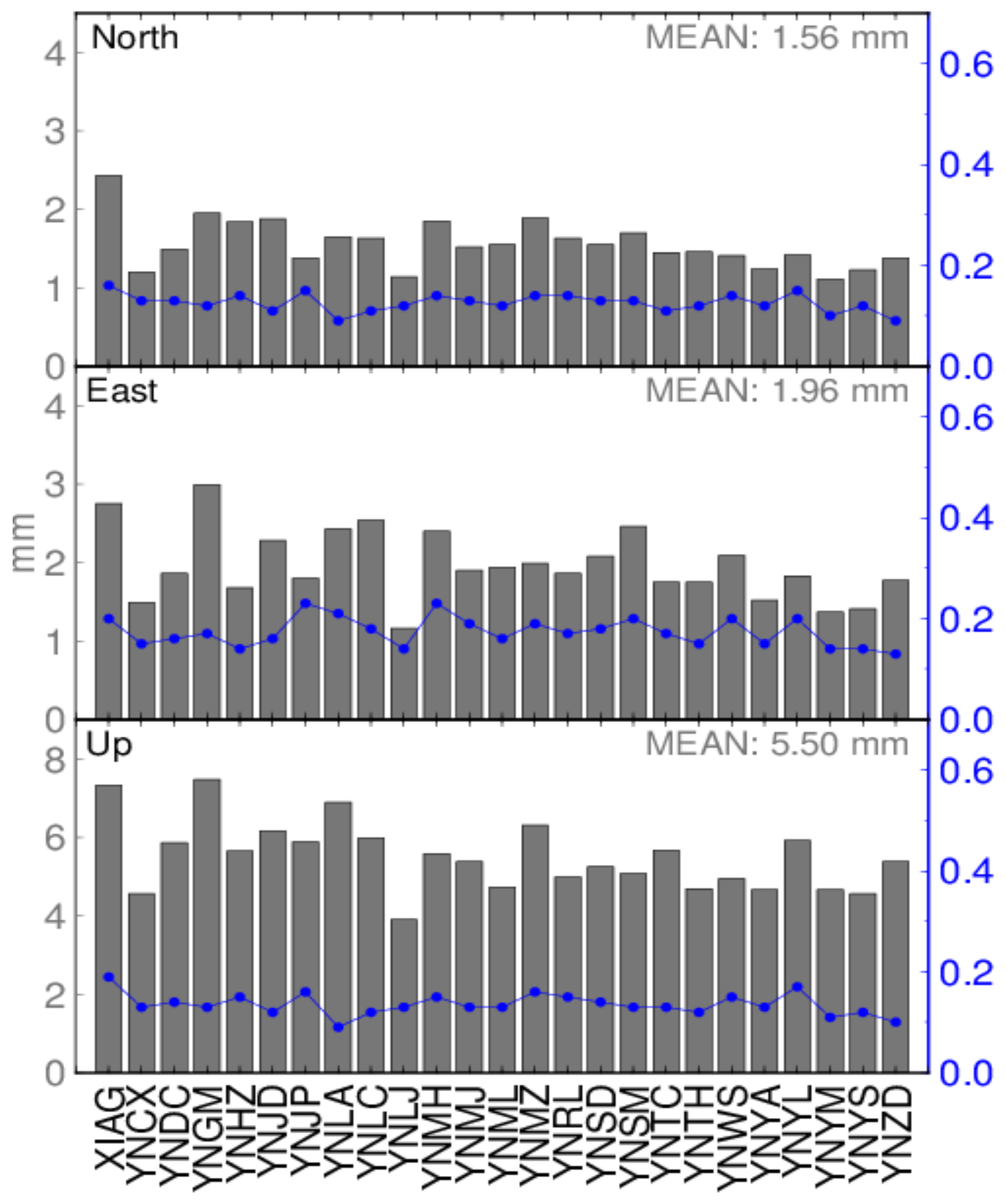
The standard deviations of unit weight derived from Equation (5) are shown in gray bars for all stations in Figure 2. We can see from Figure 2 that the standard deviations of Up components were significantly larger than the other two components. Moreover, for the same coordinate component, the standard deviations of unit weight were different for different stations and the mean values for North, East and Up components were 1.56 mm, 1.96 mm and 5.50 mm, respectively. This illustrates that it is unreasonable that unit weight adopted for each station at each epoch be used in forming covariance in PCA. Additionally, the standard deviation of weight factors is shown in blue in Figure 2. The mean standard deviation of the weight factor was 0.13, 0.17 and 0.14 for North, East and Up, respectively. We can see that the weight factor in East had the largest variation among the three components, while North ranked the least.
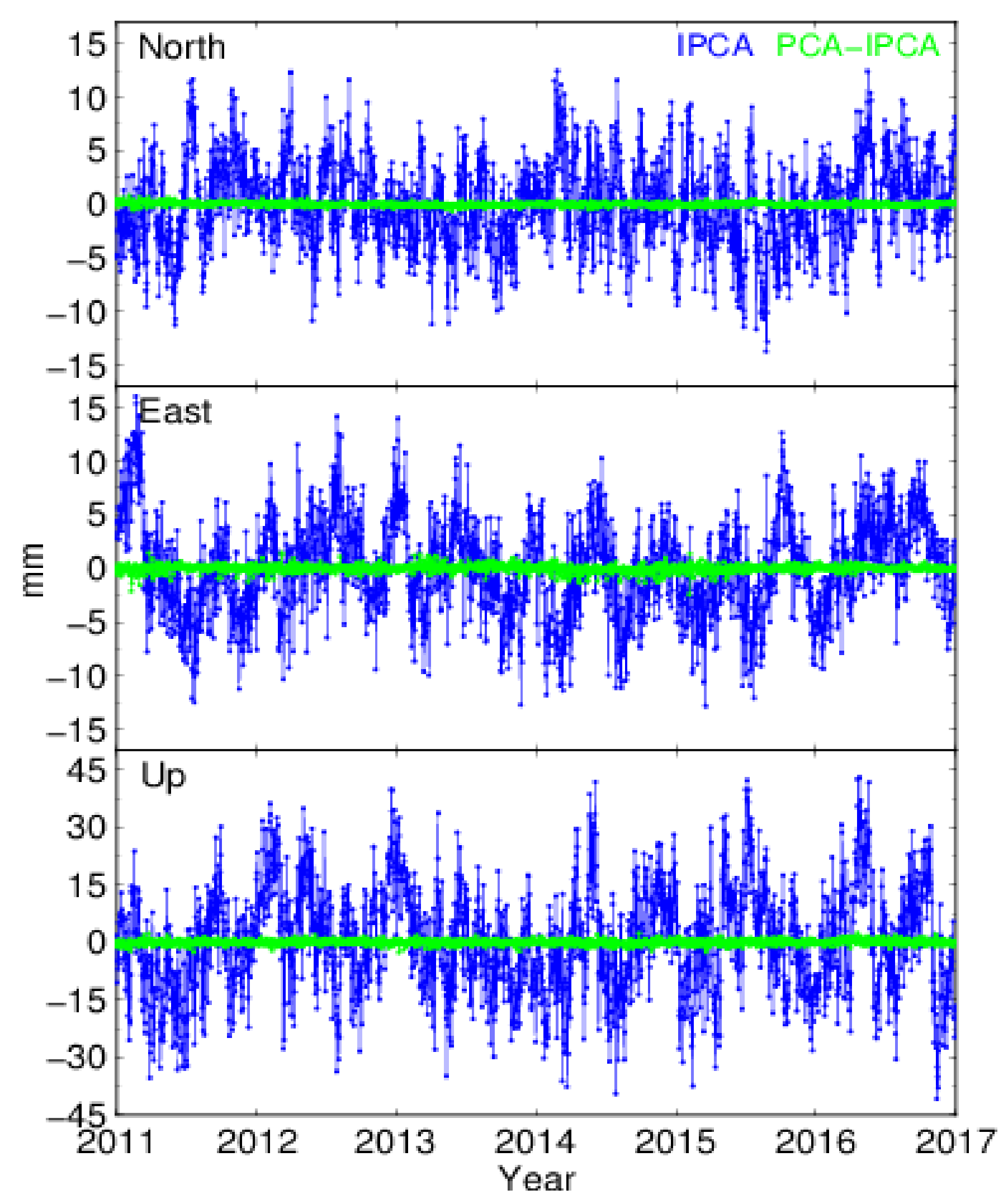
The eigenvectors showed that the spatial responses of only the first PC were consistent; therefore, the responses derived from PCA and IPCA are depicted in Figure 3. We can see that the spatial responses derived from IPCA were different to those from PCA, for the three components. The mean responses from PCA and IPCA were 73.69% and 74.63% for North, 55.17% and 54.28% for East, and 69.96% and 68.16% for Up. Their maximum relative differences were 4.30% (North) and 6.13% (Up) at XIAG station, and 6.25% (East) at YNLA station. The mean relative differences were 1.28%, 1.46% and 1.84% for North, East and Up, respectively. The first PC derived from IPCA and the difference between PCA and IPCA are shown in Figure 4, with blue and green colors, respectively. We can see that differences did exist and the mean absolute differences were 0.11 mm, 0.22 mm and 0.45 mm, respectively, for North, East and Up components.
Analysis of CME showed that it consisted of white and flicker noise and that the flicker noise was dominant, as shown in Table 1. Moreover, the proportion of flicker noise in CME derived from IPCA was slightly larger than that derived from PCA.
After CME was filtered out, the average errors of residual time series of each station were calculated with Equation (12) for PCA and Equation (13) for IPCA, as follows:
where is the CME extracted with PCA; is the CME extracted with IPCA; and is the weight for each epoch in each site in Equation (3). Since the weight is determined by Equations (4) and (5), average errors computed by Equations (12) and (13) are comparable. A smaller average error means that CME is better filtered out.
Figure 5 presents the average errors of all 25 stations before and after spatiotemporal filtering via PCA and IPCA, as well as the relative improvement of IPCA with respect to PCA. It revealed that after spatiotemporal filtering, average error was reduced for all stations and all coordinate components, and IPCA perform better than PCA for all coordinate components at all stations, especially for East component at YNJP station, which had an improvement of up to 13%. For PCA, the mean reductions of 25 stations were 15.84%, 10.86% and 14.32% for North, East and Up components, respectively. While for IPCA, the mean reductions were 18.23%, 15.42% and 18.25%. Thereby, the reductions of IPCA relative to PCA were about 2.39%, 4.56% and 3.93% for North, East and Up components, respectively. The correspondent relative improvements for North, East and Up components were 2.99%, 4.97% and 4.54%. In addition, the rank of the three components in relative improvements was consistent with that of the mean standard deviation of the weight factor in Figure 2. The correlations of improvement and standard deviation of the weight factor were 0.29, 0.76 and 0.47 in North, East and Up, respectively. The relative improvement was dependent on the standard deviation of the weight factor to some extent. In fact, it can verify the necessity of consideration of formal errors in spatiotemporal filtering, especially when formal errors are significantly inhomogeneous.
Since flicker noise was dominant in CME [28], flicker noise before and after spatiotemporal filtering is shown in Figure 6. We can see from Figure 6 that flicker noise reduced significantly after the removal of CME, regardless of whether PCA or IPCA employed. Average reductions were 34.93, 24.43, and 36.99% for PCA, and 34.96, 24.62 and 37.01% for IPCA. Hence, IPCA performed slightly better than PCA in removing common mode flicker noise.
4. Synthetic Time Series Analysis
To further test and verify the performance of the IPCA approach, simulations were carried out in this section. Firstly, eight stations were randomly selected from the above 25 stations. The CME of Up component extracted with PCA in Section 3 and the formal errors series of the selected eight stations were employed. In synthetic time series, the extracted CME of the selected stations is regarded as the true signal , and noise is generated according to formal errors , where i and k denote the ith station and the kth epoch. Therefore, the simulated time series can be expressed as:
Thus, in the simulated region with eight stations, the signals were spatial dependent, although noises were not. Since the true CME is known, we can compute the RMS of the extracted CME with:
where and denote the true CME and extracted CME of the ith station at the kth epoch; and is the number of epochs of the ith station. The smaller the RMS computed from Equation (15), the better the extracted CME. The RMS improvement of IPCA relative to PCA is thus:
where and denote the RMS derived by PCA and IPCA, respectively.
As follows, four cases were considered and compared. To avoid dependence on selected stations, eight stations were named as Group 1 and were randomly selected from 25 stations as follows:
- Group 1: YNDC, YNGM, YNJP, YNMZ, YNSD, YNYA, YNYM, YNYS
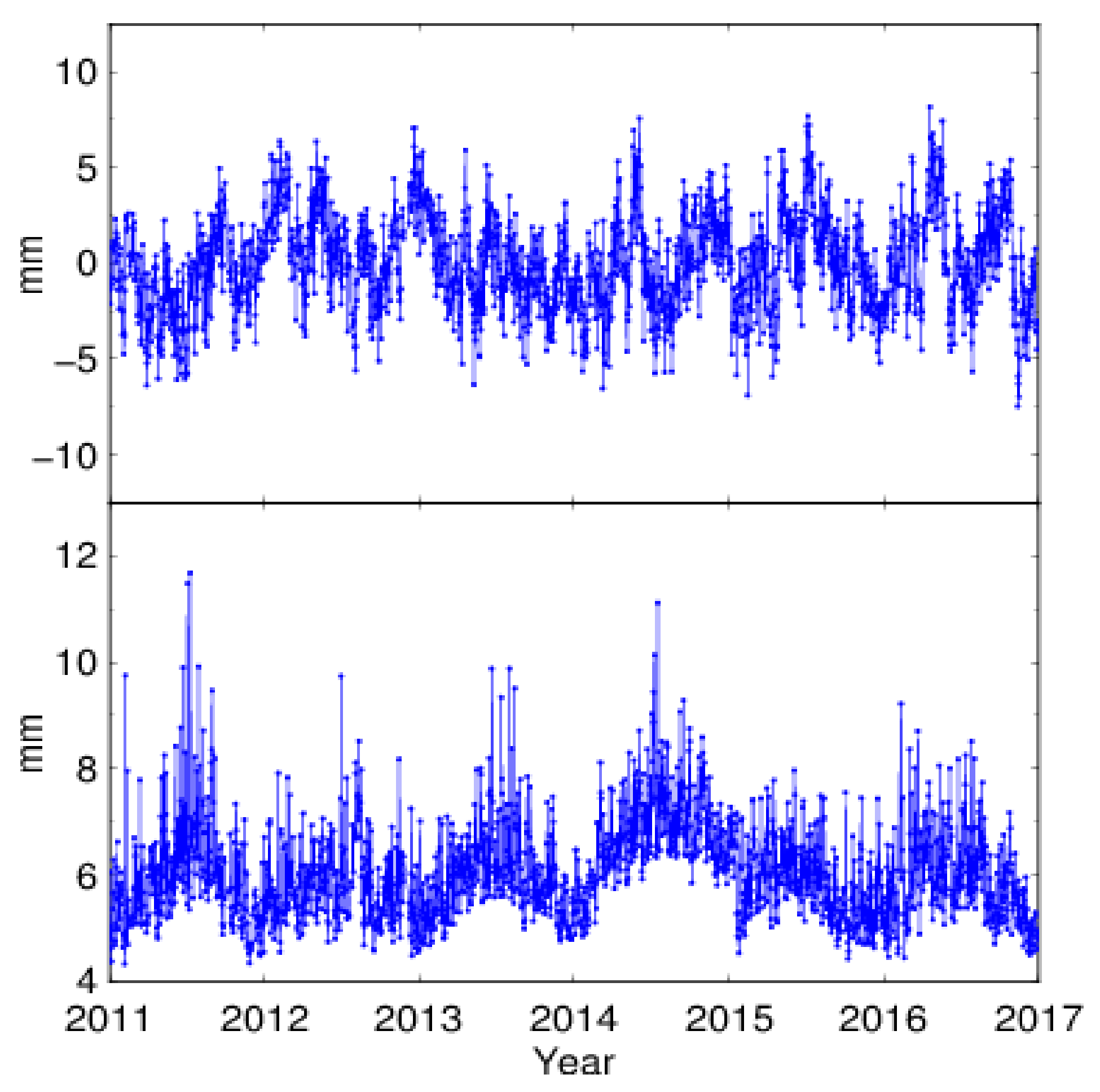
Taking the station YNDC for example, the CME and formal errors of the Up component are shown in Figure 7. We can see that the magnitude of formal errors was about 6 mm, which was even larger than that of CME. To avoid the signal being lost in the strong noise, a scale factor 0.3 was applied to the Up formal errors of all the selected stations.
Case 1: White noise and power law noise combination
Many studies indicate that not only white noise, but also colored noise exists in GNSS position time series [29,30] and that the combination of white noise and power law noise is quite common [7,8,9]. Therefore, the combination of white and power law noise was employed in noise simulation. Here, the fraction of white noise () and power spectral index () was chosen as 0.3 [9] and −0.4 [31], respectively. The amplitude of white noise () and power law noise () was determined with [32]:
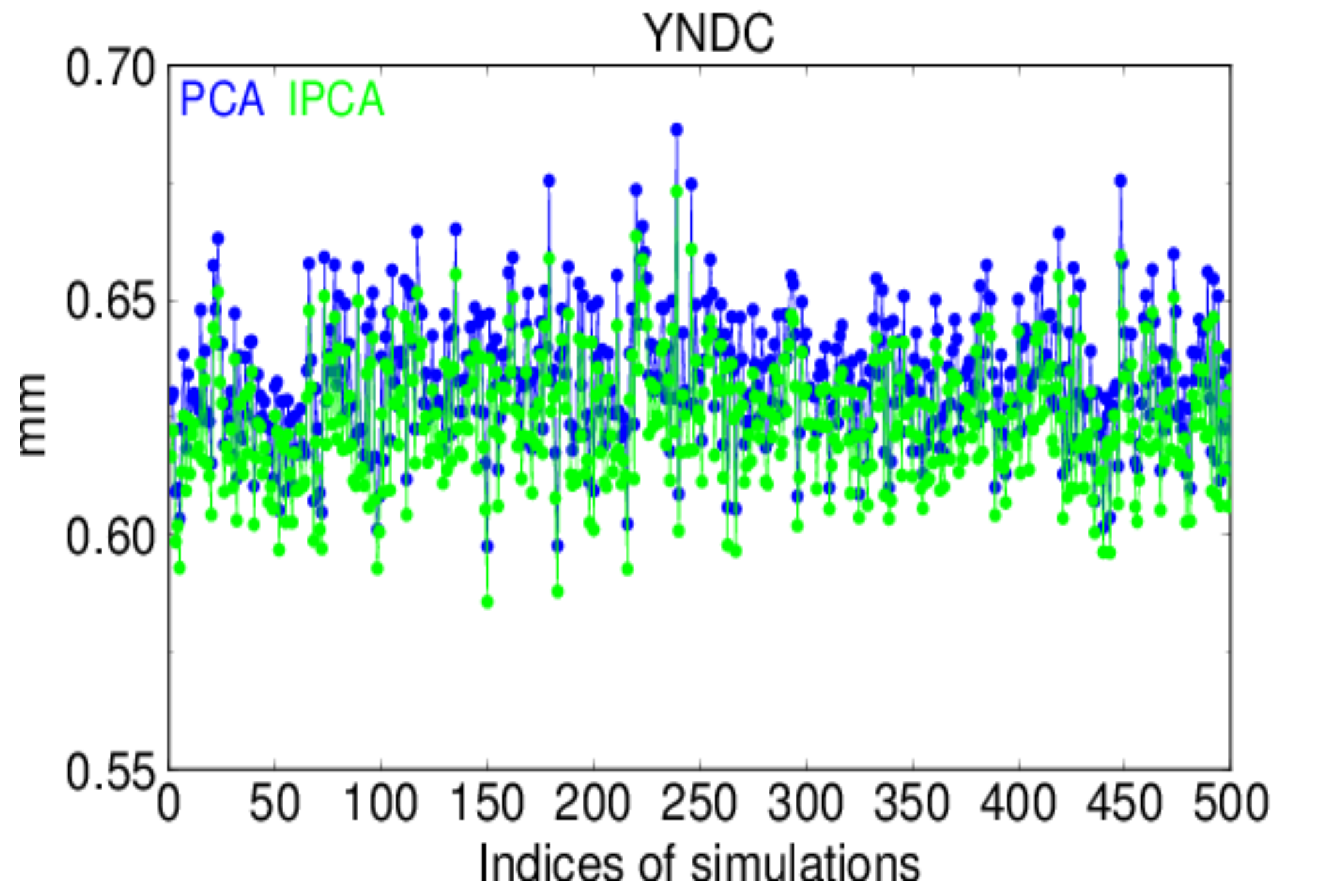
Since daily time series were investigated, dt was 1/365.25 in Equation (18). The program “simulatenoise” in Hector software [33] was used to generate the white and power law noise. Figure 8 shows the RMS values of the extracted CME signals of YNDC for each of the 500 simulations, where the RMS values for the CME derived by IPCA were smaller than those by PCA, meaning that CME by IPCA was closer to the true CME than that by PCA. The relative improvement of IPCA, with respect to PCA, was 1.41% for the mean RMS values of 500 simulations.
Case 2: Impact of different formal errors
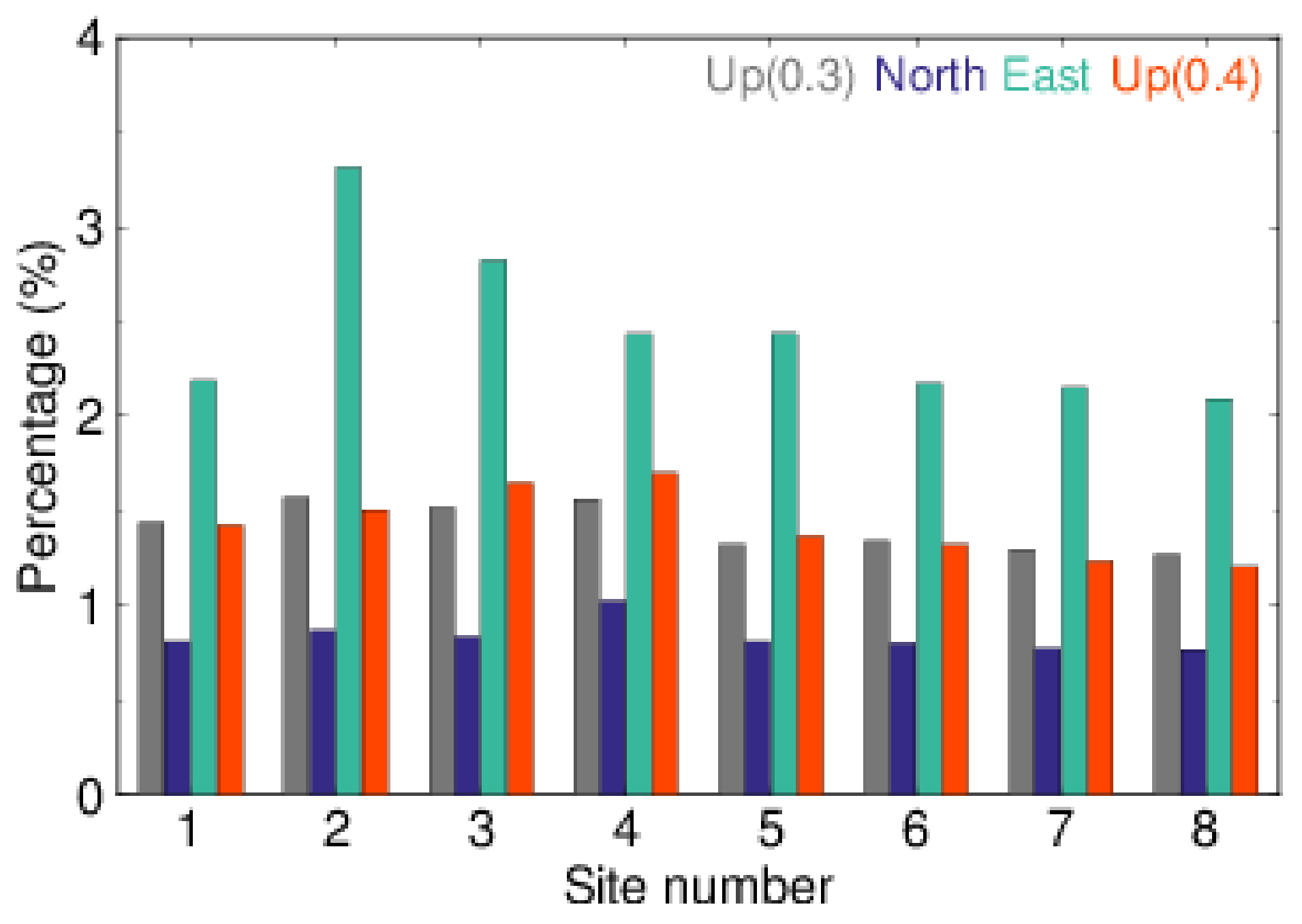
Since the CME of Up component was selected as true value, it is natural that formal errors were used to simulate noise in Case 1, although it was scaled with a factor 0.3. From Equation (4), it is apparent that formal errors, scaled or not, do not change the weight factor. In order to investigate the impacts of different formal errors, the formal errors of North and East components were also employed in the simulation of Case 2, while the same true CME was used. Figure 9 shows the formal errors of the three components of YNDC were of the same magnitude. The means of the formal errors in Figure 9 were 1.81 mm, 1.53 mm and 1.93 mm, respectively, for Up, North and East components, and the correspondent standard deviations were 0.28 mm, 0.21 mm and 0.35 mm. Similarly, the standard deviations of the three weight factors derived from the three formal errors were 0.14, 0.13 and 0.16. By using the three formal errors in Figure 9, the same 500 simulations as Case 1 were carried out and the RMS values of the derived CMEs by IPCA and PCA are shown in Figure 10, from which we can see that the RMS values derived by IPCA were all smaller than those by PCA for three formal errors. The relative improvements of IPCA relative to PCA were 1.41%, 0.83%, 2.45%, respectively, for formal errors of Up, North and East components. The relative improvements of IPCA, with respect to PCA, for all eight stations are illustrated in Figure 11, where the improvement of East formal error component ranked first among the three components for all of the eight stations. The improvements corresponding to the three formal errors were proportional to their standard deviations or the standard deviations of their weight factors. In other words, the larger the standard deviation of the weight factor, the better the IPCA performed. Since the magnitude of East formal errors was also the largest, we simulated the largest Up formal errors by scaling the original Up formal errors with a factor of 0.4 (See Table 2). The corresponding improvement is also demonstrated in Figure 11 in red. Although the Up formal errors scaled by 0.4 were larger than those of East, the improvement was still less than that of East. The reason for this was that the standard deviation of the weight factor kept unchanged, regardless of whether the Up formal errors were scaled by 0.3 or 0.4. Thus, it is reasonable to conclude that the improvement of IPCA relative to PCA was mainly related to the standard deviation of the weight factor. Moreover, the improvement for the Up formal errors scaled by 0.4 was slightly better than that scaled by 0.3; therefore, the magnitude of formal errors also impacted the performance of IPCA.
Case 3: Impact of different initial CME signal
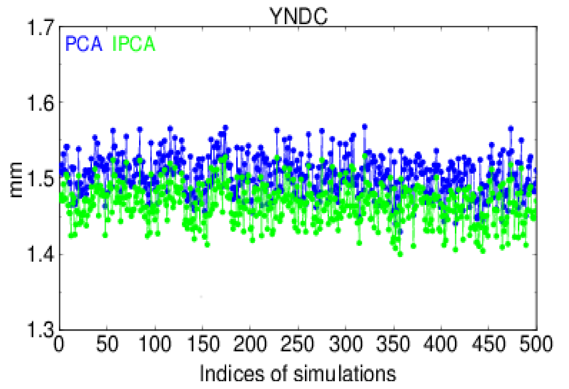
The initial CME was extracted by PCA in Cases 1–2. In order to check the impact of different initial signals on the performance of IPCA, we plotted the extracted CME signals of YNDC using the initial CME signals derived by PCA and weighted Stacking [18] in Figure 12, where the two CME signals were exactly the same. Nevertheless, as shown in Table 3, the number of iterations of PCA was less than that of weighted Stacking. It is reasonable to conclude that although the CME derived by IPCA was not related to the initial signal, the CME derived by PCA was preferred as the initial signal.
Case 4: Local effect and white, power law noise combination
Due to different environments for different stations, local effects certainly exist and may be strong in some stations or some epochs [1]. The reconstructed time series derived from the second PC to the ninth PC were, respectively, employed to simulate the local effects for the selected eight stations. Specifically, the second PC was the local effects for the first selected station, the third PC for the second station, and so on. In this case, the simulated time series is expressed with:
where represents the local effects, and the other symbols denote the same meaning as Equation (14). With the local effects considered, the RMS values of the extracted CME signals of 500 simulations are shown in Figure 13 for the station YNDC, in which the performance of IPCA was also superior to PCA. The mean RMS values of the extracted CMEs by PCA and IPCA were 1.50 mm and 1.47 mm, of which the improvement of IPCA was 2.00%.
Besides Group 1, two groups of eight stations named as Group 2 and 3 were also randomly selected from 25 stations, which are listed as follows:
- Group 2: YNMH, YNGM, YNJP, YNYL, YNSD, YNJD, YNTC, YNLC
- Group 3: YNSM, YNRL, YNYM, YNHZ, YNTC, YNWS, YNYS, YNGM
The eight stations of Group 2 and 3 were also employed for the simulation analysis of Case 1, Case 2 and Case 4. Table 4 presents the mean RMS values of the eight selected stations of extracted CME signals by PCA and IPCA, as well as the improvements of IPCA, with respect to PCA. In Case 2, the same true CME, but different formal errors were employed, where Up, North, East denoted the formal errors of Up (scaled by 0.3), North and East, respectively. The analysis of Up, in Case 2, was the same as with Case 1, which was anticipated given all the simulated parameters were the same. We can see that all the mean RMS values by IPCA were smaller than those by PCA. The relative reduction of mean RMS values ranged from 1.35% to 3.93%. It is reasonable to conclude that IPCA outperformed PCA in extracting CME, regardless of whether local effects were considered or not.
5. Discussion
Spatiotemporal filtering is a necessary step to improve the precision of position time series in processing regional GNSS time series data. In previous studies, different methods have been employed, such as Stacking [17], PCA [1,21] and ICA [3]. The observations in these studies were regarded as equally weighted, while in fact, the formal errors were different. The assumption of equal weight is not impractical. How to define the optimal weighting function in spatiotemporal filtering is an open question [1]. Distances, correlations and formal errors are the factors that are usually considered in generating weights [2,20,21]. In our previous work, we realized the importance of formal errors, but this research was not comprehensive [26]. The IPCA in the present research was proposed on the basis that formal errors are not related to CME.
With the removal of CME, RMS reduced by about 6.3% for the three components of the whole CMONOC network in China [3]. Relatively speaking, our study region was small, the CME was significant, and the RMS reductions were around 18% for North and Up components and 15% for the East component derived from IPCA. Meanwhile, from the noise analysis of CME we found that the temporal behavior of CME was not random, which coincides with Dong et al. [1,18]. The proportion of noise revealed that flicker noise was dominant in CME. Therefore, comparison of RMS before and after filtering was not enough [28]. Reductions in flicker noise were compared and we found that flicker noise reduced significantly, which aligns with the large proportion of flicker noise in CME. Further, local effects were common in GNSS stations, which may be due to unmodeled signals or the stations’ surroundings, such as multipath. Since stations with strong local effects may have significant spatial responses [1,3], the subsequent analysis may be biased. Therefore, the conventional approach would be to identify these stations through KLE and remove these stations first [1]. PCA is only appropriate for stations with weak local effects [1]. In the synthetic time series, weak local effects were included to test the performance of IPCA. The results confirmed its advantage over PCA in time series with local effects.
6. Conclusions
Considering the formal errors of position time series data available, IPCA was proposed in this paper for the spatiotemporal filtering of regional GNSS time series, in which formal errors were employed to construct weight factors. When formal errors were homogeneous, IPCA was reduced to PCA. The proposed IPCA was applied to process the position time series of 25 GNSS stations in the Yunnan Province. After spatiotemporal filtering, the average error of the position time series was reduced. For PCA, the average reductions were 15.84%, 10.86%, and 14.32% for the North, East and Up coordinate components, respectively. For IPCA, the correspondent average reductions were 18.23%, 15.42%, and 18.25%. The improvements of IPCA relative to PCA were 2.39%, 4.56% and 3.93%, respectively, for the three components. Moreover, this improvement was proportional to the standard deviation of the weight factor. Meanwhile, regardless of whether PCA or IPCA was employed, flicker noise was dominant in the extracted CME. To further demonstrate the advantages of IPCA relative to PCA, 500 simulations with four cases were performed and the results showed that regardless of whether local effects existed or not, IPCA outperformed PCA in terms of RMS of extracted CME signals. The mean RMS reduction of the extracted CME ranged from 1.35% to 3.93%. Additionally, analysis of the synthetic time series showed that IPCA was not dependent on the initial signal. Meanwhile, the improvement of IPCA relative to PCA was mainly related to the standard deviation of the weight factor, and somewhat related to the magnitude of formal errors. Overall, the findings from both the real and synthetic time series analysis highlight the necessity of considering formal errors and the effectiveness of the IPCA approach in spatiotemporal filtering.
Acknowledgments
This work was predominantly sponsored by the Natural Science Foundation of China (41731069 and 41474017). It was also supported by the Scientific Research Foundation of Shandong University of Science and Technology for Recruited Talents (No.2017RCJJ074) and the Shandong Provincial Natural Science Foundation, China (ZR201702210134). We acknowledge the CMONOC for providing raw position time series calculated with GAMIT (ftp://ftp.cgps.ac.cn/products/position). All figures were generated using GMT software [34].
Author Contributions
Yunzhong Shen provided the initial idea and concept; and Weiwei Li carried out the data analysis and wrote the main manuscript text.
Conflicts of Interest
The authors declare no conflict of interest.
References
- Dong, D.; Fang, P.; Bock, Y.; Webb, F.; Prawirodirdjo, L.; Kedar, S.; Jamason, P. Spatiotemporal filtering using principal component analysis and Karhunen-Loeve expansion approaches for regional GPS network analysis. J. Geophys. Res. 2006, 111. [Google Scholar] [CrossRef]
- Tian, Y.; Shen, Z. Extracting the regional common-mode component of GPS station position time series from dense continuous network. J. Geophys. Res. 2016, 121, 1080–1096. [Google Scholar] [CrossRef]
- Ming, F.; Yang, Y.; Zeng, A.; Zhao, B. Spatiotemporal filtering for regional GPS network in China using independent component analysis. J. Geod. 2017, 91, 419–422. [Google Scholar] [CrossRef]
- Ji, K.H. Transient Signal Detection Using GPS Position Time Series. Ph.D. Thesis, Massachusetts Institute of Technology, Cambridge, MA, USA, 2011. [Google Scholar]
- Schurr, B.; Asch, G.; Hainzl, S.; Hoech, A.; Palo, M.; Wang, R.; Moreno, M.; Bartsch, M.; Zhang, Y.; Oncken, O.; et al. Gradual unlocking of plate boundary controlled initiation of the 2014 Iquisque earthquake. Nature 2014, 512, 299–302. [Google Scholar] [CrossRef] [PubMed]
- Feng, L.; Hill, E.M.; Elosegui, P.; Qiu, Q.; Hermawan, L.; Banerjee, P.; Sieh, K. Hunt for slow slip along the Sumatran subduction zone in a decade of continuous GPS data. J. Geophys. Res. 2015, 120, 8623–8632. [Google Scholar] [CrossRef]
- Amiri-Simkooei, A.R. Non-negative least-squares variance component estimation with application to GPS time series. J. Geod. 2016, 90, 451–466. [Google Scholar] [CrossRef]
- Hao, M.; Freymueller, J.T.; Wang, Q.; Cui, D.; Qin, S. Vertical crustal movement around southeastern Tibetan Plateau constrained by GPS and GRACE data. Earth Planet. Sci. Lett. 2016, 437, 1–8. [Google Scholar] [CrossRef]
- He, X.; Montillet, J.P.; Fernandes, R.; Bos, M.; Yu, K.; Hua, X.; Jiang, W. Review of current GPS methodologies for producing accurate time series and their error sources. J. Geodyn. 2017, 106, 12–29. [Google Scholar] [CrossRef]
- Mao, A.; Harrision, C.G.A.; Dixon, T.H. Noise in GPS coordinate time series. J. Geophys. Res. 1999, 104, 2797–2816. [Google Scholar] [CrossRef]
- Williams, S. Error analysis of continuous GPS position time series. J. Geophys. Res. 2004, 109. [Google Scholar] [CrossRef]
- Amiri-Simkooei, A.R.; Tiberius, C.C.J.M.; Teunissen, P.J.G. Assessment of noise in GPS coordinate time series: Methodology and results. J. Geophys. Res. 2007, 112. [Google Scholar] [CrossRef]
- Shen, Y.; Li, W. Spatiotemporal signal and noise analysis of GPS position time series of the permanent stations in China. In Earth on the Edge: Science for a Sustainable Planet; International Association of Geodesy Symposia Springer: Berlin, Germany, 2014. [Google Scholar]
- Serpelloni, E.; Faccenna, C.; Spada, G.; Dong, D.; Williams, S.D.P. Vertical GPS ground motion rates in the Euro-Mediterranean region: New evidence of velocity gradients at different spatial scales along the Nubia-Eurasia plate. J. Geophys. Res. 2013, 118, 6003–6024. [Google Scholar] [CrossRef]
- Li, W.; Shen, Y. Velocity estimation of GPS base stations considering the coloured noises. J. Appl. Geod. 2012, 6, 149–157. [Google Scholar] [CrossRef]
- Gruszczynski, M.; Klos, A.; Bogusz, J. Orthogonal transformation in extracting of common mode error from continuous GPS network. Acta Geodyn. Geomater. 2016, 13, 291–298. [Google Scholar] [CrossRef]
- Wdowinski, S.; Bock, Y.; Zhang, J.; Fang, P.; Genrich, J. Southern California permanent GPS geodetic array: Spatial filtering of daily positions for estimating coseismic and postseismic displacements induced by the 1992 Landers earthquake. J. Geophys. Res. 1997, 102, 18057–18070. [Google Scholar] [CrossRef]
- Nikolaidis, R. Observation of Geodetic and Seismic Deformation with the Global Positioning System. Ph.D. Thesis, University of California, San Diego, CA, USA, 2002. [Google Scholar]
- Bogusz, J.; Gruszczynski, M.; Figurski, M.; Klos, A. Spatio-temporal filtering for determination of common mode error in regional GNSS networks. Open Geosci. 2015, 7, 140–148. [Google Scholar] [CrossRef]
- Márquez-Azúa, B.; DeMets, C. Crustal velocity field of Mexico from continuous GPS measurements, 1993 to June 2001: Implications for the neotectonics of Mexico. J. Geophys. Res. 2003, 108. [Google Scholar] [CrossRef]
- He, X.; Hua, X.; Yu, K.; Xuan, W.; Lu, T.; Zhang, W.; Chen, X. Accuracy enhancement of GPS time series using principal component analysis and block spatial filtering. Adv. Space Res. 2015, 55, 1316–1327. [Google Scholar] [CrossRef]
- Schneider, T. Analysis of incomplete climate: Estimation of mean values and covariance matrices and imputation of missing values. J. Clim. 2001, 14, 853–871. [Google Scholar] [CrossRef]
- Liu, N.; Dai, W.; Santerre, R.; Kuang, C. A MATLAB-based Kriged Kalman filter software for interpolating missing data in GNSS coordinate time series. GPS Solut. 2018, 22. [Google Scholar] [CrossRef]
- Shen, Y.; Li, W.; Xu, G.; Li, B. Spatiotemporal filtering of regional GNSS network’s position time series with missing data using principal component analysis. J. Geod. 2014, 88, 1–12. [Google Scholar] [CrossRef]
- Jolliffe, I.T. Principal Component Analysis, 2nd ed.; Springer: Berlin/Heidelberg, Germany, 2002. [Google Scholar]
- Li, W.; Shen, Y.; Li, B. Weighted spatiotemporal filtering using principal component analysis for analyzing regional GNSS position time series. Acta Geod. Geophys. 2015, 50, 419–436. [Google Scholar] [CrossRef]
- Langbein, J.; Bock, Y. High-rate real-time GPS network at Parkfield: Utility for detecting fault slip and seismic displacements. Geophys. Res. Lett. 2004, 31. [Google Scholar] [CrossRef]
- Santamaría-Gómez, A.; Mémin, A. Geodetic secular velocity errors due to interannual surface loading deformation. Geophys. J. Int. 2015, 202, 763–767. [Google Scholar] [CrossRef]
- Bogusz, J.; Klos, A. On the significance of periodic signal in noise analysis of GPS station coordinate time series. GPS Solut. 2016, 20, 655–664. [Google Scholar] [CrossRef]
- Deng, L.; Jiang, W.; Chen, H.; Zhu, Z.; Zhao, W. Study of the effects on GPS coordinate time series caused by higher-order ionospheric corrections calculated using the DIPOLE model. Geod. Geodyn. 2017, 8, 111–119. [Google Scholar] [CrossRef]
- Klos, A.; Bogusz, J.; Figurski, M.; Gruszczynski, M. Error analysis for European IGS stations. Stud. Geophys. Geod. 2015, 60. [Google Scholar] [CrossRef]
- Bos, M.S.; Fernandes, R.M.S. Hector User Manual 1.6; University of Beira Interior: Covilhã, Portugal, 2016. [Google Scholar]
- Bos, M.S.; Fernandes, R.M.S.; Williams, S.D.P.; Bastos, L. Fast error analysis of continuous GNSS observations with missing data. J. Geod. 2013, 87, 351–360. [Google Scholar] [CrossRef]
- Wessel, P.; Smith, W.H.F.; Scharroo, R.; Luis, J.; Wobbe, F. Generic mapping tools: Improved version released. EOS Trans. AGU 2013, 94, 409–410. [Google Scholar] [CrossRef]
Figure 1.
Location of the selected 25 GNSS stations in YunNan Province.
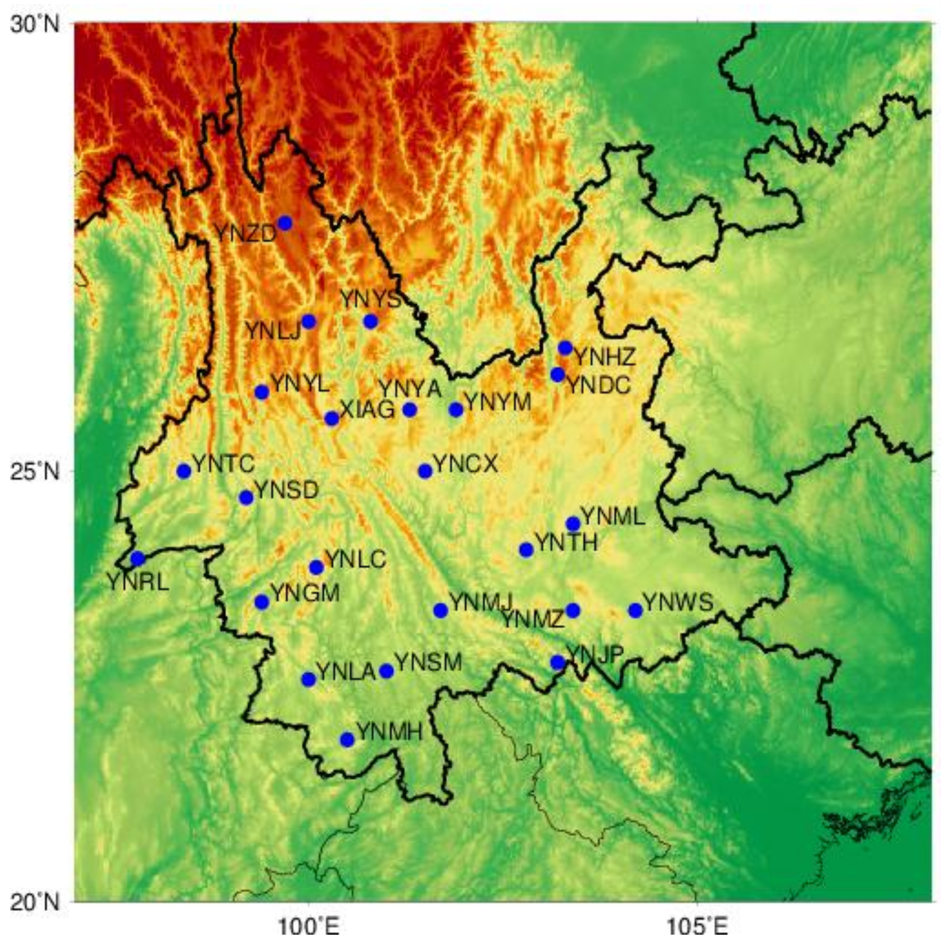
Figure 2.
Standard deviation of unit weight (gray bar) and weight factor (blue line) for each station.
Figure 2.
Standard deviation of unit weight (gray bar) and weight factor (blue line) for each station.

Figure 3.
Spatial response of Principal Component Analysis (PCA) and Improved Principal Component Analysis (IPCA) for three components.
Figure 3.
Spatial response of Principal Component Analysis (PCA) and Improved Principal Component Analysis (IPCA) for three components.
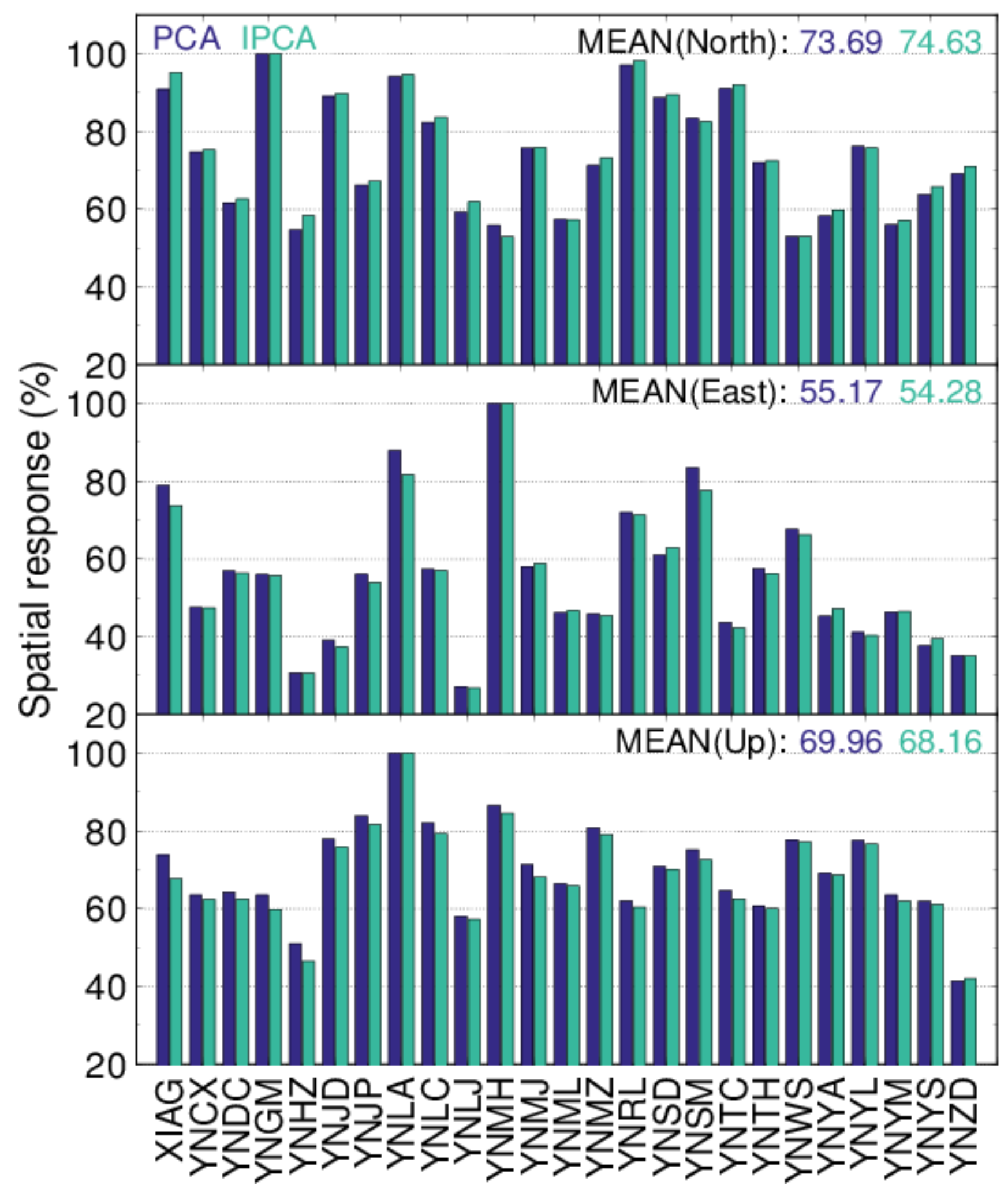
Figure 4.
First PC from IPCA and the difference between PCA and IPCA for three components.

Figure 5.
Average error and relative improvement for three components.
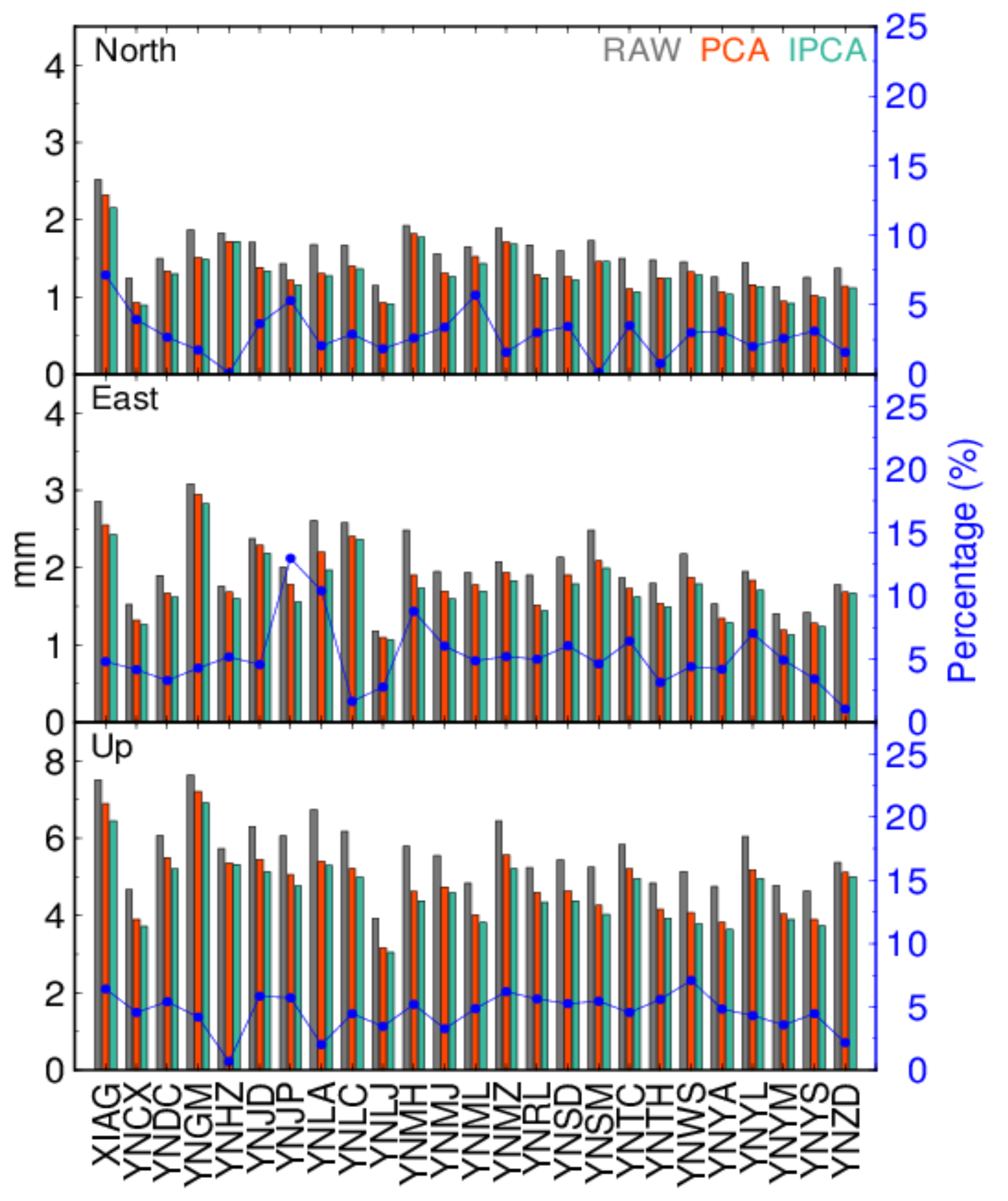
Figure 6.
Flicker noise magnitude for three components.
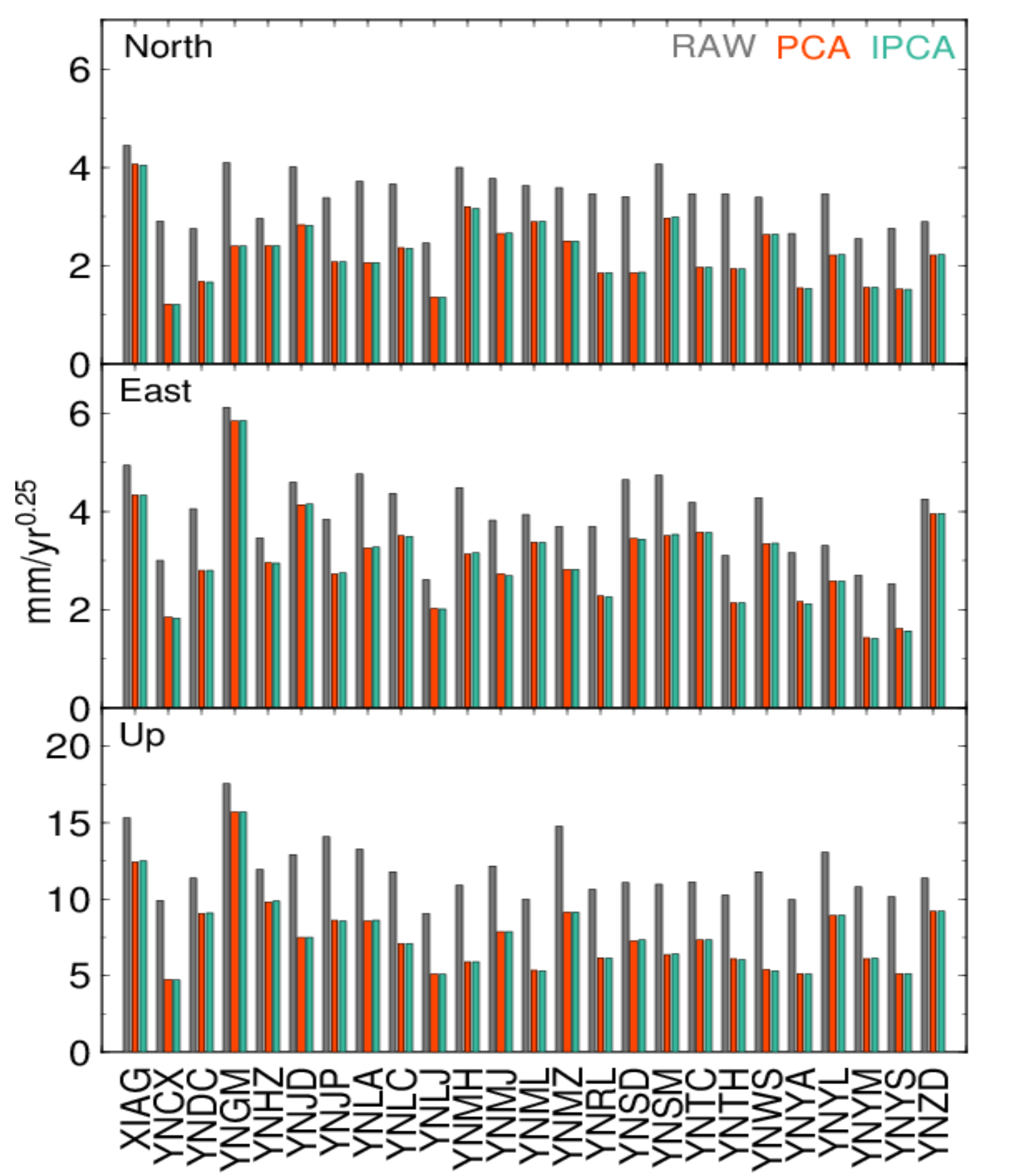
Figure 7.
CME (top panel) and formal errors (bottom panel) of YNDC site in Up.

Figure 8.
Root mean square (RMS) with white and power law noise combination considered.

Figure 9.
Formal errors of three components (Up scaled by 0.3).
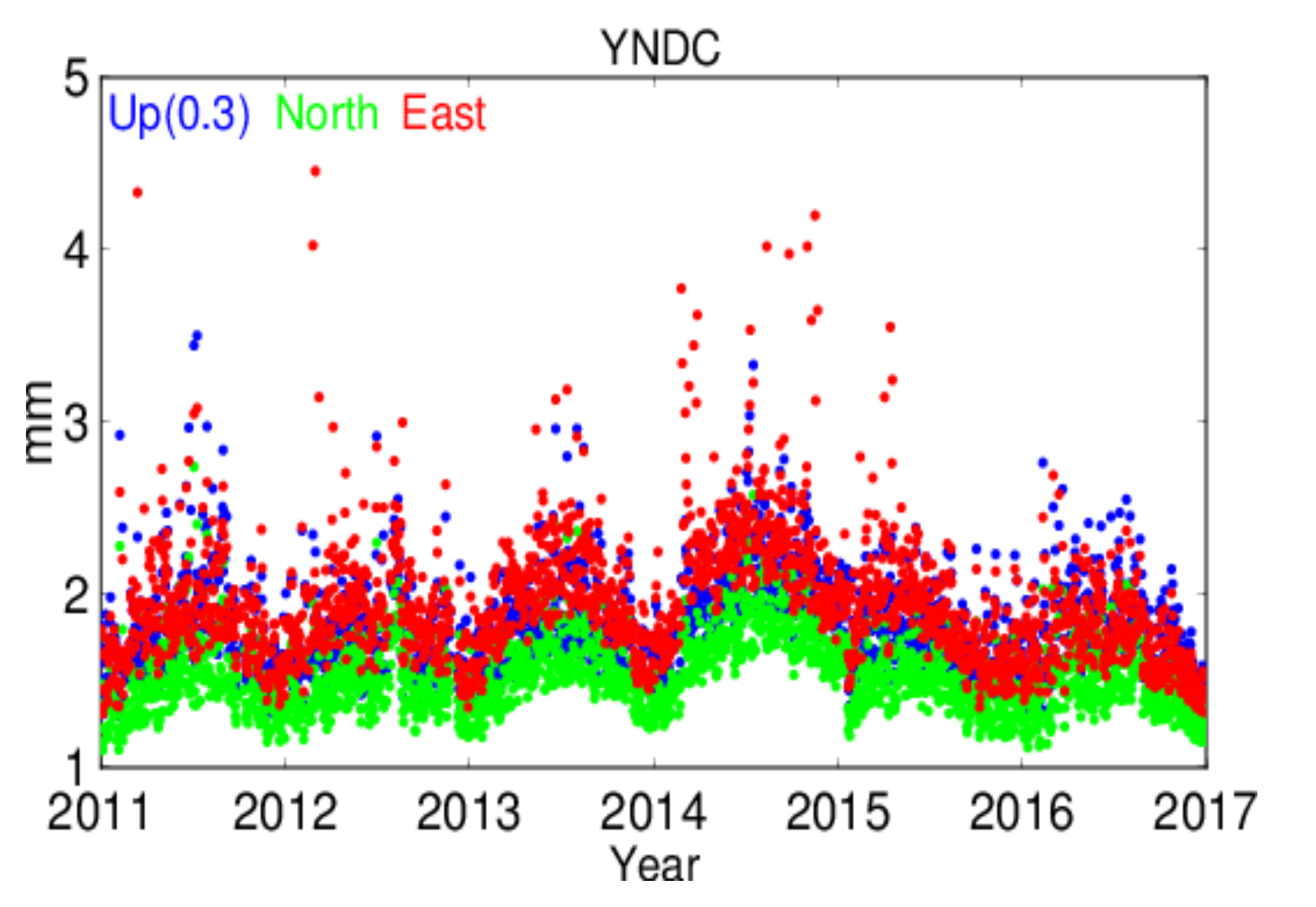
Figure 10.
RMS values of extracted CME with different formal errors.
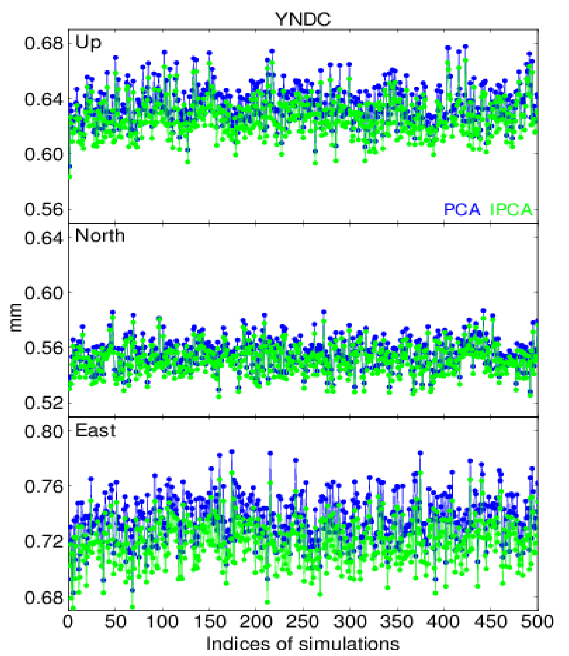
Figure 11.
Relative improvement of IPCA relative PCA in eight stations.

Figure 12.
Extracted CME of YNDC with different initial signals.
Figure 13.
RMS with local effects considered of YNDC.

Table 1.
The proportion of white and flicker noise in Common Mode Error (CME).
| White Noise | Flicker Noise | |||
|---|---|---|---|---|
| PCA | IPCA | PCA | IPCA | |
| North | 0.212 | 0.211 | 0.788 | 0.789 |
| East | 0.329 | 0.315 | 0.671 | 0.685 |
| Up | 0.100 | 0.094 | 0.900 | 0.906 |
Table 2.
Mean formal errors (mm) of three components (Up scaled).
| Station | 1 | 2 | 3 | 4 | 5 | 6 | 7 | 8 |
|---|---|---|---|---|---|---|---|---|
| Up(0.3) | 1.81 | 2.30 | 1.84 | 1.97 | 1.63 | 1.44 | 1.42 | 1.40 |
| Up(0.4) | 2.42 | 3.07 | 2.45 | 2.63 | 2.17 | 1.92 | 1.90 | 1.87 |
| North | 1.53 | 1.99 | 1.43 | 1.95 | 1.60 | 1.27 | 1.13 | 1.26 |
| East | 1.93 | 3.14 | 1.98 | 2.11 | 2.20 | 1.58 | 1.42 | 1.46 |
Table 3.
Iteration statistics of using different initial CME signals in 500 simulations.
| Number of Iterations | 4 | 5 | 6 | 7 | 8 | 9 | 10 | 11 | |
|---|---|---|---|---|---|---|---|---|---|
| Number of simulations | PCA | 3 | 241 | 198 | 58 | 0 | 0 | 0 | 0 |
| weighted Stacking | 0 | 0 | 0 | 0 | 42 | 118 | 237 | 103 | |
Table 4.
Mean RMS (mm) and relative improvement (%) in each test.
| Case 1 | Case 2 | Case 4 | |||||||||
|---|---|---|---|---|---|---|---|---|---|---|---|
| PCA | IPCA | Up | North | East | PCA | IPCA | |||||
| PCA | IPCA | PCA | IPCA | PCA | IPCA | ||||||
| Group 1 | RMS | 0.69 | 0.68 | 0.69 | 0.68 | 0.61 | 0.60 | 0.82 | 0.80 | 1.99 | 1.93 |
| Imp | 1.45 | 1.75 | 1.64 | 2.50 | 3.00 | ||||||
| Group 2 | RMS | 0.74 | 0.73 | 0.74 | 0.73 | 0.67 | 0.66 | 0.96 | 0.93 | 1.78 | 1.71 |
| Imp | 1.35 | 1.35 | 1.49 | 3.13 | 3.93 | ||||||
| Group 3 | RMS | 0.65 | 0.64 | 0.65 | 0.64 | 0.62 | 0.61 | 0.86 | 0.84 | 0.72 | 0.71 |
| Imp | 1.54 | 1.54 | 1.61 | 2.32 | 1.39 | ||||||
© 2018 by the authors. Licensee MDPI, Basel, Switzerland. This article is an open access article distributed under the terms and conditions of the Creative Commons Attribution (CC BY) license (http://creativecommons.org/licenses/by/4.0/).
Share and Cite
MDPI and ACS Style
Li, W.; Shen, Y. The Consideration of Formal Errors in Spatiotemporal Filtering Using Principal Component Analysis for Regional GNSS Position Time Series. Remote Sens. 2018, 10, 534. https://doi.org/10.3390/rs10040534
AMA Style
Li W, Shen Y. The Consideration of Formal Errors in Spatiotemporal Filtering Using Principal Component Analysis for Regional GNSS Position Time Series. Remote Sensing. 2018; 10(4):534. https://doi.org/10.3390/rs10040534
Chicago/Turabian StyleLi, Weiwei, and YunZhong Shen. 2018. "The Consideration of Formal Errors in Spatiotemporal Filtering Using Principal Component Analysis for Regional GNSS Position Time Series" Remote Sensing 10, no. 4: 534. https://doi.org/10.3390/rs10040534
Note that from the first issue of 2016, this journal uses article numbers instead of page numbers. See further details here.