Inferring Water Table Depth Dynamics from ENVISAT-ASAR C-Band Backscatter over a Range of Peatlands from Deeply-Drained to Natural Conditions

Abstract

Water table depth (WTD) is one of the key variables controlling many processes in peatlands. Reliable WTD estimates based on remote sensing data would advance peatland research from global-scale climate monitoring to field-scale ecosystem management. Here, we evaluate the relationship between ENVISAT Advanced Synthetic Aperture Radar (ASAR) C-band backscatter (σ°) and in situ observed WTD dynamics over 17 peatlands in Germany covering deeply-drained to natural conditions, excluding peatlands dominated by forest or inundation periods. The results show increasing σ° with shallower WTD (=wetter conditions), with average temporal Pearson correlation coefficients of 0.38 and 0.54 (-) for natural (also including disturbed and rewetted/restored states) and agriculturally-used drained peatlands, respectively. The anomaly correlation further highlights the potential of ASAR backscatter to capture interannual variations with values of 0.33 and 0.43 (-), for natural and drained peatlands. The skill metrics, which are similar to those for evaluations of top soil moisture from C-band over mineral soils, indicate a strong capillary connection between WTD and the ‘C-band-sensitive’ top 1–2 cm of peat soils, even during dry periods with WTD at around −1 m. Various backscatter processing algorithms were tested without significant differences. The cross-over angle concept for correcting dynamical vegetation effects was tested, but not superior, to constant incidence angle correction.

1. Introduction

Many functions of peatlands strongly depend on the thickness of the aerated peat layer and its soil water content. Peatlands, defined in this context as lands with peat soil, act as source or sink for greenhouse gases [1] and nutrients [2], moderate flood events [3], and are important for the conservation of biodiversity [4] and the agricultural productivity for which they have been drained in many areas of the world [5].

Neglecting the saturated part of the capillary fringe, which is typically only a few centimeters thick, the thickness of the aerated zone corresponds to the water table depth (WTD). Since the WTD can be measured at low costs with pipes, it is the most frequently available hydrological variable for characterizing peatlands from drained to naturally-wet conditions. However, although WTD measurements appear to be simple, they also have a lot of potential shortcomings which need to be taken into consideration (see, e.g., Section 4.5.2 of the practical guide of [6]). Pipes installed in thin peat layers often cut through potentially confining soil layers into the underlying aquifer, consequently measuring the water pressure in the aquifer rather than the one in the peat layer. Pipes installed in natural peatlands with an oscillating soil surface either measure the absolute water level (deeply-anchored pipes), or the water level relative to the peat surface (anchored in the upper part of the peat), or some undefined value in between (not anchored). Another difficulty is the spatial representativeness of the measured WTD, because natural peatlands, in particular, typically have a considerable microrelief, i.e., the distance from the ground surface to the water table varies in space. The alternative of measuring soil moisture rather than WTD is even more problematic in peatlands. The loose organic ‘soil’ material complicates ground sampling, anchoring of sensors, and the calibration of typical sensors [7].

The difficulties associated with ground measurements along with the need for a global monitoring of peatlands to better estimate their impact on climate change [8] are a strong motivation to develop remote sensing methods that allow reliable and representative estimates of soil moisture and WTD dynamics over peatlands. In natural peatlands, several studies have taken advantage of the possible capillary dependence of near-surface-soil or vegetation moisture on water table depth to indirectly infer information about water table depth from multi-spectral reflectance [9,10], and passive [11] and active [8] microwave measurements (Figure 1). To our knowledge, there are no studies about the potential of microwave remote sensing to monitor WTD over peatlands drained for agricultural use. Nevertheless, drained peatlands are important as hot spots of greenhouse gas emissions in several countries [12], and will be included in our study.

For natural peatlands, spectral reflectance of typical peatland vegetation has been shown to be very sensitive to WTD changes. The characteristics of spectral changes, however, vary strongly with detailed vegetation composition [10], limiting the applicability of the optical approach for lack of information on detailed vegetation composition at larger scales. Unlike optical data, microwave observations have the advantage that they can penetrate the vegetation, and are available without sun illumination, which is a constraint in higher latitudes. Kim et al. [11] reported high correlation coefficients (R = 0.8) between WTD observations and soil moisture retrievals from passive L-band microwave remote sensing (SMAP) for the Great Dismal Swamp. Although the study included only a single water level monitoring site, and even if the retrieval algorithm was not optimal for peat soils, the high correlation indicates a high potential for measuring hydrological changes over extensive peatland areas with coarse resolution observations from passive microwave remote sensing. Active microwave data is available at finer spatial resolution. However, the interpretation of backscatter over peatlands, or wetlands in general, is difficult due to specular reflection and/or double-bounce backscattering on vegetation structures when part of the area is inundated [13,14,15,16]. Kasischke et al. [8] reported for sites with a sparse tree cover in an Alaskan peatland that ERS SAR C-band backscatter (VV-polarized) decreased with higher water levels during inundation periods due to specular reflection, while there was no correlation for the drier water level range. In contrast, Kim et al. [11] presented in their study over the Great Dismal Swamp a high positive correlation between backscatter (HH-polarized, C-band Radarsat-1, and L-band ALOS PALSAR) and WTD for non-inundation periods, but the comparison was based on only one water level station within the peatland. Kim et al. [11] additionally used InSAR coherence to delineate flooded areas and temporal InSAR analysis to estimate surface water level changes, improving the interpretation of radar data during periods with inundation.

In the aforementioned studies, backscatter coefficients σ° have not been corrected for the influence of seasonally-changing vegetation. In our study, we will evaluate the effect of vegetation corrections to C-band backscatter values to study whether such corrections could improve the link between backscatter values and WTD. Backscatter over vegetated surfaces is strongly influenced by volume scattering in the vegetation layer, which can completely attenuate the sensitivity of the radar signal to soil moisture depending on wavelength, polarization, viewing geometry, and aboveground biomass [17]. In general, bare soil backscatter contributions decrease with increasing incidence angle (θ). In contrast, the contribution from the vegetation canopy itself is assumed to be fairly uniform over a large range of incidence angles [18]. Based on the different incidence angle dependencies of soil and vegetation, Wagner et al. [18] proposed that depending on the relative contributions of soil and vegetation at different incidence angles, vegetation growth can either increase or decrease the overall backscatter. As a consequence, the authors assumed that there exist soil moisture-dependent cross-over points for which the influence of a changing vegetation biomass is minimal (Figure 2).

Based on this theoretical consideration, they established a semi-empirical concept to account for the dynamical vegetation effect on backscatter intensity to improve soil moisture estimates. The concept uses the cross-over angles at dry and wet reference states (θ_d and θ_w, with θ_d < θ_w due to decreasing sensitivity with increasing aboveground biomass) in a normalization approach (with the equations given in Section 3.1.3) that is based on the assumptions that (i) for a certain vegetation state, σ° linearly depends on soil moisture; and that (ii) the incidence angle dependency changes over the year only due to changes of aboveground biomass and not due to soil moisture. Incidence angle dependency is parameterized directly from backscatter observations at multiple incidence angles (e.g., ERS scatterometers or Advanced Scatterometer (ASCAT)) typically by a second order Taylor series. The slope and curvature parameterize the vegetation dynamics for every day of the year and for every grid point.

For mineral soils of the Iberian Peninsula, Wagner et al. [18] established the two cross-over angles θ_d = 25° and θ_w = 40°, which have not been modified in subsequent applications since then. Since its introduction, the concept is routinely applied to generate soil moisture estimates from radar data [19]. Since soil moisture products have only been validated for mineral soils [20] due to the lack of easily accessible and good quality data from peat soils, it is unclear whether the concept can also improve the correlation between backscatter and soil moisture and/or water level over peatlands.

In this study, we evaluate, for the first time, the potential of the European Space Agency’s ENVISAT Advanced Synthetic Aperture Radar (ASAR) C-band backscatter time series to estimate WTD dynamics over the whole range from drained and agriculturally-used to near-natural and unused peatlands. To this end, we take advantage of a recently-compiled, quality-checked comprehensive dataset of peatland water levels in Germany [21]. The ENVISAT ASAR backscatter data are selected because scatterometer backscatter observations (as e.g., available from ASCAT) have a too coarse a spatial resolution to be analyzed over smaller peatlands for which the water table depth monitoring information is typically available. The ENVISAT ASAR data have a finer spatial resolution, as data are collected at a sub-antenna footprint resolution by means of range and Doppler discrimination [22]. Furthermore, we will test whether different ENVISAT backscatter processing algorithms can improve the interpretation of the data. These processing options include incidence angle normalization and vegetation correction using the cross-over angle concept, with a possible optimization of cross-over angles over peatlands.

2. Data

2.1. ENVISAT-ASAR Backscatter Intensity

For our study area of peatlands across Germany, we used a dataset acquired by ENVISAT ASAR (C-band, 5.3 GHz) in Wide Swath (WS) and VV polarization mode between July 2005 and April 2012. All imagery used in this study is in vertical transmit-vertical receive (VV) polarization. Although horizontal transmit–horizontal receive (HH) polarization penetrates more through vertical components of the vegetation layer and, thus, is expected to contain more information about soil moisture and water table depth [11], we decided to evaluate VV images as HH coverage was insufficient over our German dataset of peatland water table depths (see Figure 6-4 and 6-5 in [23]). A total number of 2100 WS Level 1B files was downloaded for the study area. At every point in space, time series were composed of backscatter values acquired at various incidence angles ranging from 15° to 44° and in descending (~8:00 am local time) and ascending (~8:00 pm local time) orbital nodes. Acquisition was heterogeneous in time and space leading to varying data frequency over our study sites. On average, one backscatter value was available every six to seven days.

In order to improve the information on position and velocity of the observation platform, precise “Doppler Orbitography and Radiopositioning Integrated by Satellite” (DORIS) orbits [24] were used. The downloaded ASAR scenes were multilooked with seven looks in both azimuth and range directions in order to decrease the influence of speckle. At the resulting pixel spacing of 525 m, ASAR WS data has a radiometric resolution of ca. 0.2 dB [25] in comparison to >1 dB at the original spatial resolution of 150 m [26]. A finer resolution would have better captured the small-scale variability from field to field that is often present in German peatlands, e.g., due to differences in land-use and land management, as well as spatially-variable water-management, often small scale restoration measures or different levels of disturbance in natural peatlands. Speckle noise was, however, still too high at finer resolutions. The scenes were then geocoded using the Range-Doppler approach [27] and a digital elevation model (DEM) from the Shuttle Radar Topography Mission [28]. Backscatter coefficients σ° were obtained by radiometric normalization against projected local incidence angles, θ, derived from the DEM. The geocoded scenes were then resampled using bilinear interpolation to a common grid with a pixel spacing of 30”, which corresponds to ca. 500 m at the equator. All σ° values were log-transformed and expressed in units of dB. Likewise, projected local incidence angles were retained in the same database for the subsequent analysis of θ–σ° relationships.

2.1.1. Environmental Scene Filter

Scenes that were obviously unsuitable for the comparison with water level time series were excluded. Weather station data from the German Weather Service were used to filter data for snow or frozen conditions. A soil temperature (5 cm depth) threshold of 2.0 °C was applied to filter frozen conditions using data from a weather station closest to each water level validation data point. Further, all scenes with precipitation >20 mm at the day of the acquisition were excluded. Precipitation events can cause disturbances in microwave observations [29] and, in our study, would additionally cause temporary disequilibrium between top soil moisture and water table depth. In total, 25% of the scenes were filtered by the environmental scene filter.

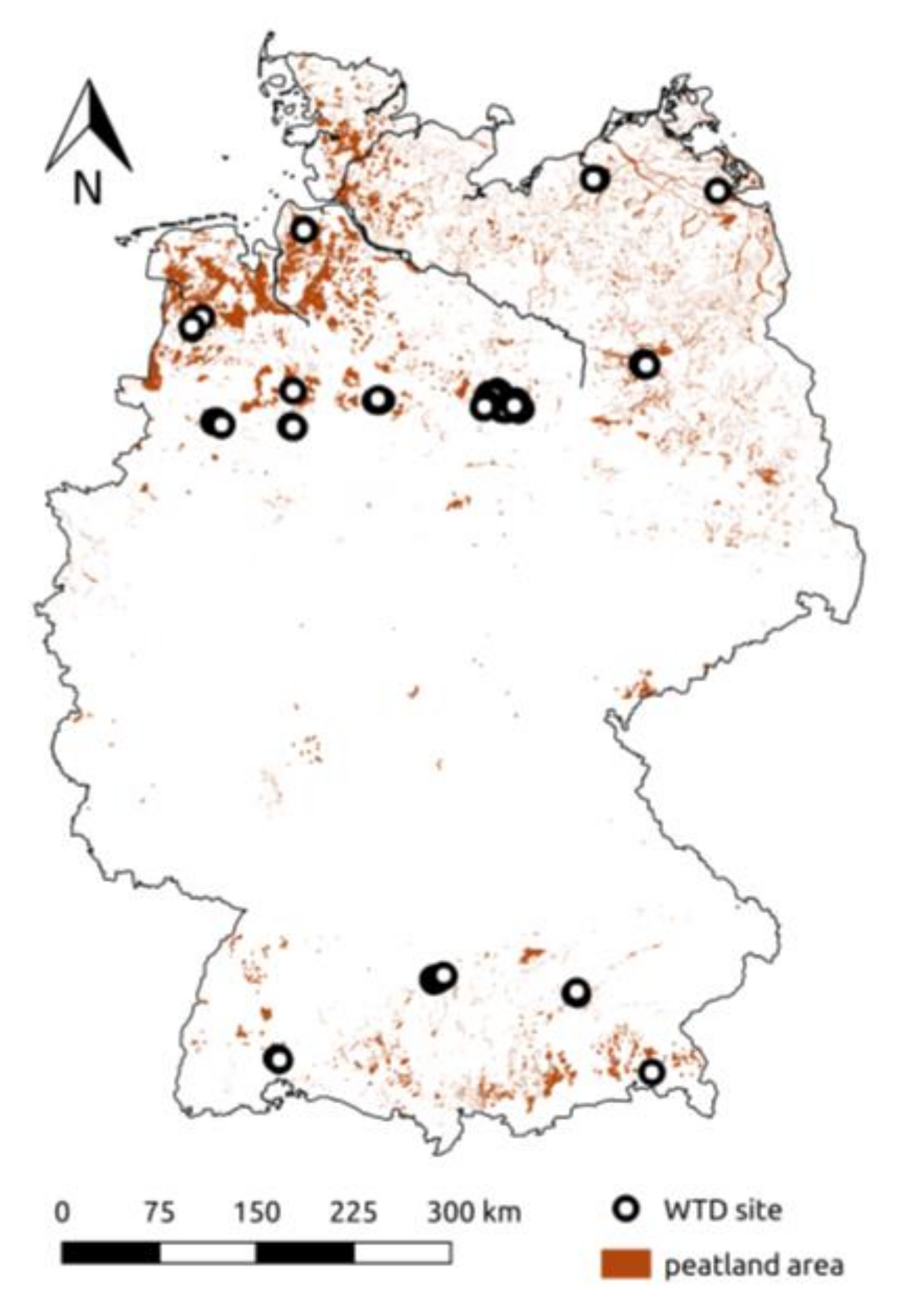
2.2. Ground-Based WTD Data in Peatlands

Ground-based WTD data was taken from the national dataset for Germany presented and used in Bechtold et al. [21]. This dataset was compiled from multiple sources including local agencies, non-governmental organizations, universities, and consultants for a nation-wide statistical upscaling of the annual mean WTD and greenhouse gas emissions over German peatlands including other organic soils with lower soil organic carbon content (SOC), but still meeting the definition of organic soils according to IPCC [30]. Quality assessment of the dataset, in particular included checks assuring that phreatic water levels, and not piezometric pressure heads, of underlying aquifers were measured. Originally, the dataset included 1094 dip wells from 53 peatlands and covered data between 1988 and 2012, good for a total of 7000 years of data. The time series include continuous logger time series, as well as discontinuous (weekly to monthly or even bi-monthly) manual time series. Part of the discontinuous manual time series could be interpolated to continuous daily time series using the process-based statistical time series model Menyanthes of von Asmuth et al. [31] using precipitation and evapotranspiration data from the German Weather Service. We used the interpolated data when the time series model explained more than 70% of the observed variance. For time series that could not be satisfactorily interpolated with the time series model, we assumed the same water table depth three days before and after the manual reading when there was less than 10 mm cumulative precipitation and evapotranspiration before and after the reading.

Only part of the processed time series was suited for the comparison with the backscatter data. Most WTD time series were excluded due to a limited overlap (<3 years) with the ENVISAT ASAR period and a temporal resolution of less than biweekly measurements after the above-mentioned possible interpolation. Furthermore, monitoring wells located in ASAR pixels that included >30% forest cover, >30% mineral soils, or >30% open water (use of processed land cover data from [21]) were also excluded from the dataset due to the strong influence of these land cover types that would disturb our analysis. Furthermore, a few sites that were dominated by inundation periods were excluded. The in situ locations were divided into two major peatland classes for further analysis: drained and natural peatlands. Sites were classified based on the dominant class within a 500 m buffer around the in situ sites, again using the land cover classes from Bechtold et al. [21] based on the German Digital Landscape Model (ATKIS Basis DLM). The land cover classes that contributed to the drained (agriculturally-used) class were “Grassland” (59%), “Wet grassland (1%)”, and “Arable land (8%)”, and to the natural (not agriculturally-used) class were “Wet unused peatland” (25%), “Unused peatland” (1%), and “Reed” (1%). The natural class included well-preserved peatlands, more disturbed peatlands, and peatlands that have been restored to some degree starting from variably-disturbed states (e.g., due to peat-mining) by rewetting measures that took place before the study period. In general, the class name ‘natural’ does not imply that in all cases peat-forming peatland species dominated the footprint (quantitative information not available). ‘Natural’ indicates that, compared to the agriculturally-used drained peatlands, there was a rather natural development of vegetation on the peat soil in the footprint depending on the site-specific conditions (e.g., moisture) that resulted from some peatland ecosystem management. The final WTD dataset used in our study comprised data from 179 monitoring wells (drained: 126, natural: 53) from 17 different peatland complexes (drained: 11, natural: 9; i.e., some peatlands contained both classes) in Germany (Figure 3).

3. Methodology

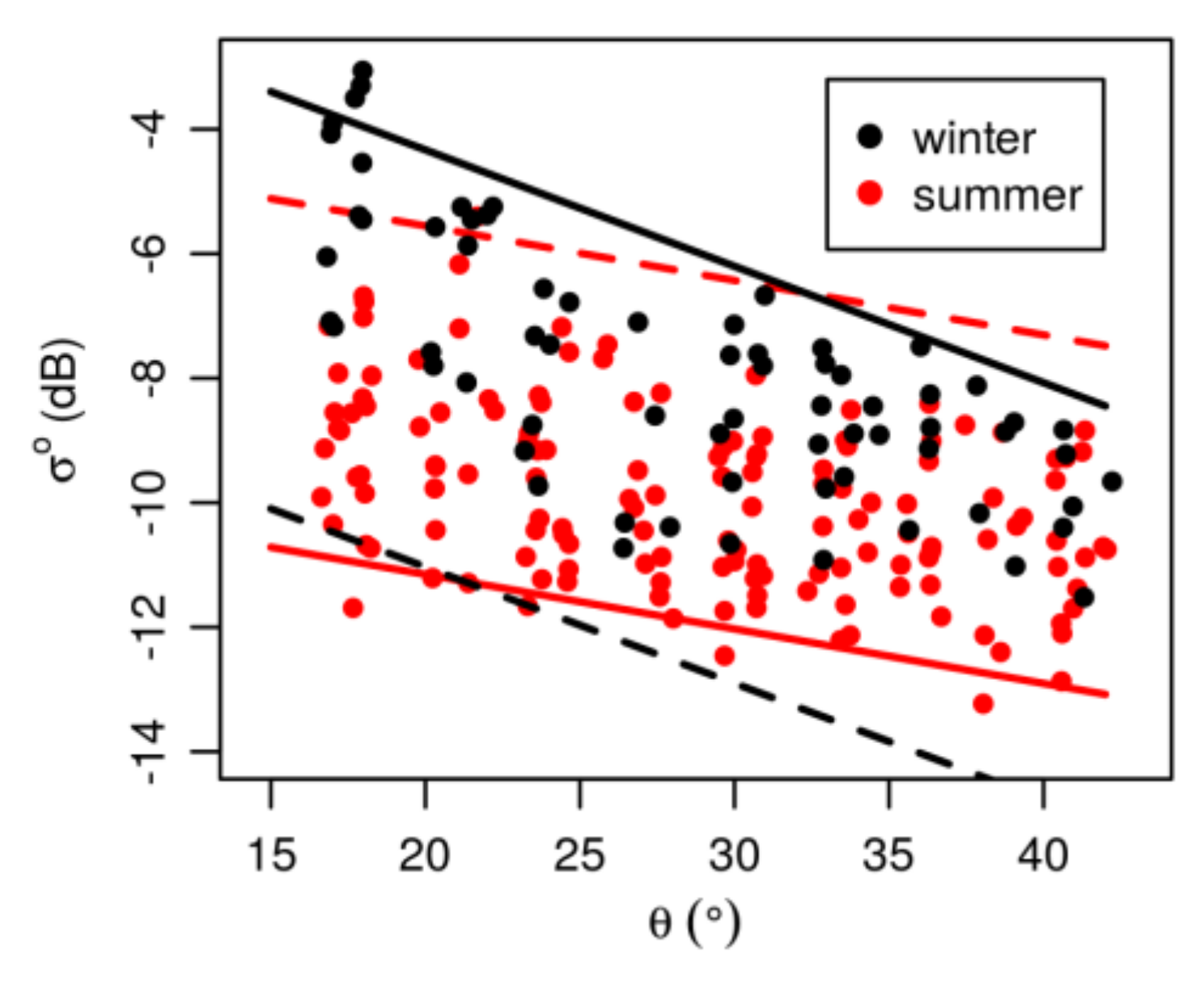
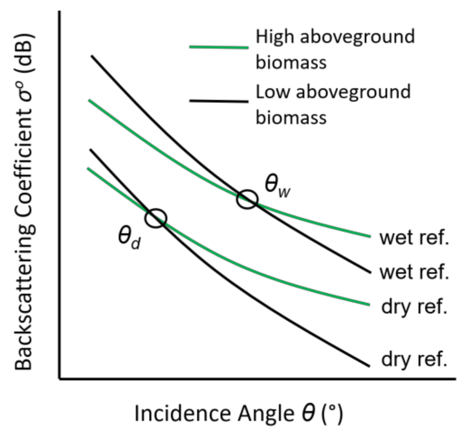
3.1. Incidence Angle Normalization and Cross-Over Angle Concept

In the following sections (Section 3.1.1 through Section 3.1.3), the methods that were used to account for incidence angle and dynamical vegetation effects on backscatter are presented. The configurations that were finally tested are sometimes a combination of these methods and will be listed in Section 3.2.

3.1.1. Linear Normalization with Constant Site-Specific Slope Parameter (β_const)

The simplest form to account for incidence angle dependency of backscatter is the linear normalization [32]. The curvature of the dependency is typically neglected for the moderate incidence angle range of ASAR data [22]. Accordingly, in this scheme, all ASAR backscatter values are normalized to a common incidence angle of θ_r = 40°:

$${\sigma }_{{\theta }_r}^{\circ }={\sigma }_{\theta }^{\circ }+{\beta }_{const}\cdot \left({\theta }_r-\theta \right)$$

(1)

where β_const (dB/degree) is the site-specific constant slope parameter of the linear regression between ASAR σ° (dB) and θ (degree) across all times, i.e., independent of water table, soil moisture, or vegetation conditions.

3.1.2. Dynamical Site-Specific Slope (β_doy)

In order to take advantage of the cross-over angle concept, there must be knowledge about how β changes over time. The ERS-1 and ERS-2 Scatterometer and the Metop ASCAT measure σ° simultaneously at multiple angles and allow derivation of slope values at a specific time step, which are commonly called the local slopes [33]. Local slopes of a moving window are then used to derive the slope and curvature of a second-order Taylor time series for each day of the year as climatology or, more recently, also as continuous multi-annual time series [33]. Local slopes cannot be derived from ENVISAT ASAR, as σ° of only one incidence angle is available at a time.

In order to obtain a temporally-variable incidence angle dependency for each pixel of the processed ASAR data, we conducted a linear regression between multi-year σ° and $\theta$ for the data within windows around a “day of year” (doy), yielding a climatology of a linear incidence angle dependency. Our windows used the data from all years to average out the intra- and interannual wetness differences, while ensuring sufficient angular coverage (see ‘Weighing’ below). As in Loew et al. [32], the curvature was neglected. The window size was variable over time due to the varying data frequency. Based on manual inspection of the obtained climatology time series, we decided on a window size that included at least 30 data points covering both the low and high incidence angles. The window size is typically a trade-off between obvious noise and information about the temporal variability of the variable of interest (here the “day of year–specific” slope parameter, i.e., β_doy). At the coarse scale (ASCAT: 12.5 km), incidence angle dependency typically shows a clear seasonal pattern with shallow slopes (small negative β) in summer with denser vegetation and steep slopes (larger negative β) in winter with less biomass [34]. At the fine scale, which is, in our case, dominated by a mixture of grasslands and natural peatland vegetation, this might be often less systematic. Grasslands are typically cut once or several times per year leading to temporally low vegetation biomass in summer periods. As cut dates may vary considerably from year to year, it was not our goal to capture cut dynamics with our climatology time series.

Weighing

Due to the irregular temporal coverage of acquisitions with low and high incidence angles, artefacts would have occurred when one edge of the averaging window covered a period with typically deeper or shallower water table depths with either only low or high incidence angles. For example, if the early summer period of an averaging window that began in the late winter was only covered by acquisitions made at high incidence angles, the high incidence angle backscatter was biased towards lower values (due to deeper water tables in the early summer) which leads to an overestimation of the slope. This effect was reduced by a weighing scheme. We fitted a data density function (Epanechnikov kernel with ‘SJ’ automatic smoothing bandwidth, R package stats v3.4.3, [35]) for each window around a specific doy to both the low and the high incidence angle range and used the density functions to weigh the data of the other incidence angle range.

Ascending/Descending Incidence Angle Dependency

For several sites, we observed considerable differences between σ° from ascending and descending node. Nevertheless, due to relatively limited data for our window average approach, we decided to fit a single incidence angle dependency describing both ascending and descending data simultaneously. Here, again, irregular temporal coverage of incidence angles and different coverage for ascending and descending led to artefacts, e.g., when there was systematic difference between the orbital nodes and one of the nodes only covered either the low or the high incidence angle range. These artefacts were reduced by fitting a linear mixed effects model (R package lme4 v1.1-15 [36]) with a random intercept to the data in each window with the ascending/descending node as a random effect.

3.1.3. Cross-Over Angle Concept

The cross-over angle concept was implemented according to Wagner et al. [18]. In the following, it is presented for the simplified linear case, i.e., without curvature correction. In a first step, the temporally-variable slope parameter, β_doy, is used to normalize all ${\sigma }_{{\theta }_{\mathrm{i}}}^{\circ }(i)$ observed at time step i and arbitrary θ_i to the cross-over angles θ_d and θ_w:

$${\sigma }_{{\theta }_d}^{\circ }\left(i\right)={\sigma }_{{\theta }_i}^{\circ }\left(i\right)+{\beta }_{doy}\cdot \left({\theta }_d-{\theta }_i\right)$$

(2)

$${\sigma }_{{\theta }_w}^{\circ }\left(i\right)={\sigma }_{{\theta }_i}^{\circ }\left(i\right)+{\beta }_{doy}\cdot \left({\theta }_w-{\theta }_i\right)$$

(3)

Normalized ${\sigma }_{{\theta }_d}^{\circ }\left(i\right)$ and ${\sigma }_{{\theta }_w}^{\circ }\left(i\right)$ were then used to calculate the dry and wet reference backscatter (${\sigma }_{{\theta }_d}^d$ and ${\sigma }_{{\theta }_w}^w$) at the corresponding cross-over angles by averaging the 10% lowest and highest backscatter values, respectively. Note that the dry and wet reference backscatter values are constant over time at the cross-over angles, whereas for other incidence angles they are vegetation-dependent and, thus, change with time. The time-dependent dry and wet reference backscatters are calculated for an arbitrarily-defined final reference angle (θ_r = 40°) at which all backscatter data will be compared:

$${\sigma }_{{\theta }_r}^d\left(doy\right)={\sigma }_{{\theta }_d}^d+{\beta }_{doy}\cdot \left({\theta }_r-{\theta }_d\right)$$

(4)

$${\sigma }_{{\theta }_r}^w\left(doy\right)={\sigma }_{{\theta }_w}^w+{\beta }_{doy}\cdot \left({\theta }_r-{\theta }_w\right)$$

(5)

Finally, ${\sigma }_{{\theta }_r}^d\left(doy\right)$ and ${\sigma }_{{\theta }_r}^w\left(doy\right)$ are used to scale all θ_r-normalized backscatter values ${\sigma }_{{\theta }_r}^{\circ }\left(i\right)$ using:

$${\sigma }_{{\theta }_r,c}^{\circ }(i)=\frac{{\sigma }_{{\theta }_r}^{\circ }(i)-{\sigma }_{{\theta }_r}^d\left(doy\right)}{{\sigma }_{{\theta }_r}^w\left(doy\right)-{\sigma }_{{\theta }_r}^d\left(doy\right)}\times \left(\overline{{\sigma }_{{\theta }_r}^w}-\overline{{\sigma }_{{\theta }_r}^d}\right)+\overline{{\sigma }_{{\theta }_r}^d}$$

(6)

where ${\sigma }_{{\theta }_r,c}^{\circ }(i)$ is the backscatter at θ_r and corrected for vegetation dynamics, and $\overline{{\sigma }_{{\theta }_r}^d}$ and $\overline{{\sigma }_{{\theta }_r}^w}$ are the temporally-averaged dry and wet reference backscatter coefficients at θ_r. The quotient in Equation (6) corresponds to the scaling between 0 and 1 of Wagner et al. [18]. The second part of Equation (6) scales values to the average σ° range at θ_r = 40° to make the magnitude of ${\sigma }_{{\theta }_r,c}^{\circ }$ comparable across sites. Note that the effect of vegetation on the absolute level of ${\sigma }_{{\theta }_r,c}^{\circ }$ is not corrected by the cross-over angle concept.

3.2. Comparison of Backscatter with WTD Observations

3.2.1. Application of Different Processing Configurations

We processed the ASAR backscatter time series in four different ways, and compared them against the ground-based WTD time series to evaluate the temporal agreement. The four different processing configurations were:

• UNCOR: Uncorrected backscatter time series neglecting the incidence angle dependency
• CONST: Constant slope normalization (Section 3.1.1) [32]
• COASCAT: Application of the cross-over concept using site-specific β_doy and curvature climatology from the corresponding ASCAT pixels at 12.5 km grid spacing (provided by TU Vienna). Approach as presented in Section 3.1.3, but additionally including curvature values for normalization (see Wagner et al. [18]).
• COASAR: Application of the cross-over concept using site-specific slope climatology β_doy derived from ASAR data (Section 3.1.2).

We compared the four different processing configurations for both the ascending and descending node. The slopes were determined using both ascending and descending simultaneously, but we evaluate skill metrics separately for both orbital nodes due to observed systematic differences between the two nodes.

3.2.2. Skill Metrics

The different processing configurations were compared using temporal correlation statistics, i.e., time series correlation coefficient between σ° and WTD. Pearson correlation coefficients (R) were determined for the original time series. Anomaly Pearson correlation coefficients (anomR) were determined for time series from which the site-specific multiyear, two-months-smoothed average was removed. Thus, the anomR skill level reflects the capability of the C-band to monitor water levels that are higher or smaller than usual for that period. Confidence intervals (CI) were calculated for a 95% confidence level, taking into account the temporal autocorrelation (as in [37]). CIs were derived for each WTD monitoring location, and then first averaged for each peatland complex, as done for the values of R and anomR as well. Finally, overall R, anomR, and CIs were computed by averaging across peatland complexes. For CI, the average value was further divided by the square root of the number of peatland complexes, under the assumption that each peatland complex adds independent information [37].

4. Results

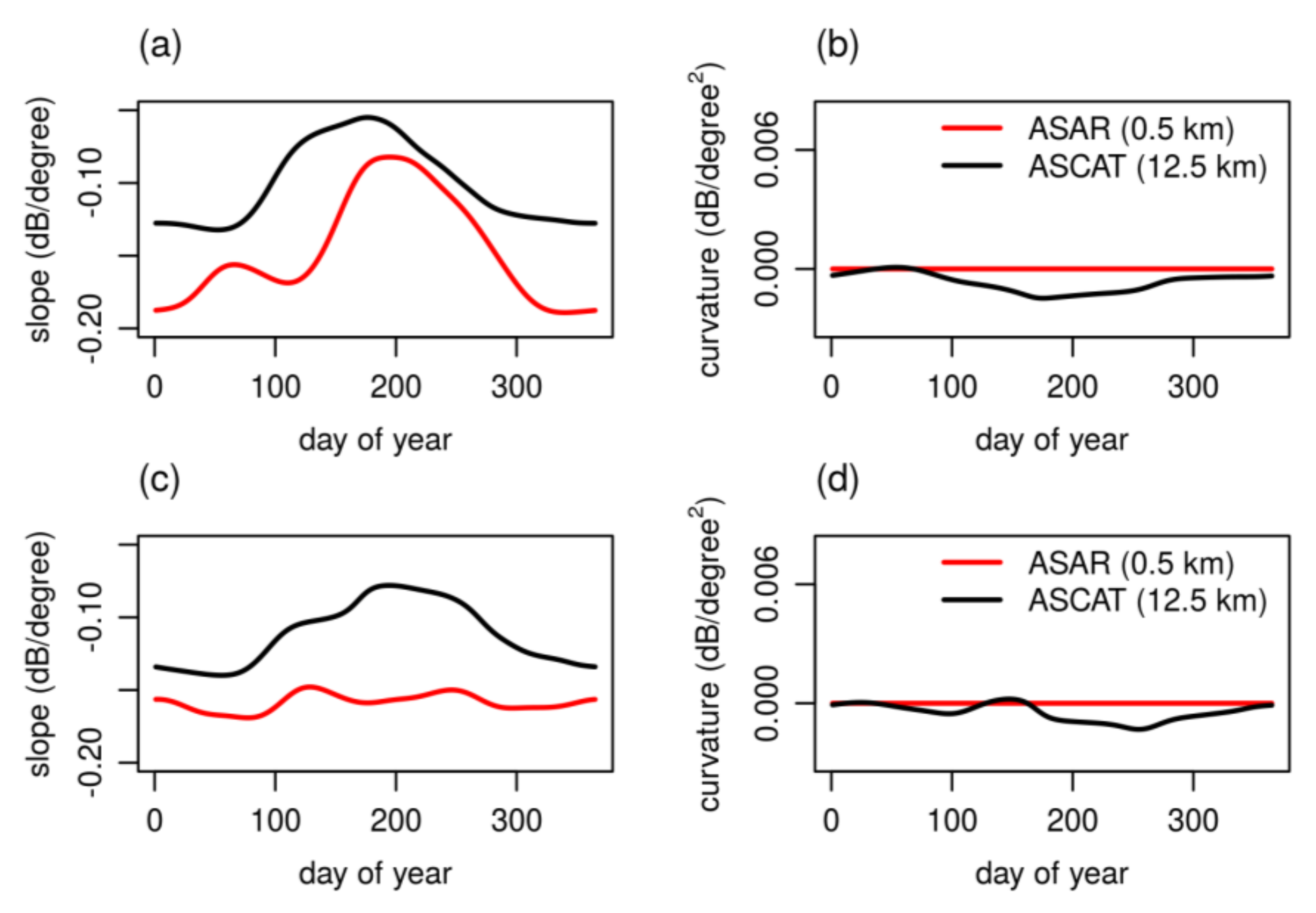
4.1. Climatology of Site-Specific Slope Parameter Based on ASAR Data

The site-specific slope time series derived from the 0.5 km ASAR data differed considerably from the 12.5 km resolution ASCAT slope climatology time series. The yearly average of the climatological ASAR slopes were steeper (−0.153 dB/degree) than ASCAT slopes (−0.098 dB/degree) across all our peatland locations. The value is consistent with the average of the site-specific constant slopes (Section 3.1.1) which was −0.155 dB/degree. Figure 4 shows examples of times series from two locations. On the one hand, there were sites (Figure 4a,b) for which the evolution in β_doy was similar for ASCAT and ASAR, with an offset towards lower (steeper) slope values for ASAR and a temporal shift of the peak value (here towards later times of the year for ASAR). On the other hand, there were also sites where the β_doy for ASCAT and ASAR showed very different dynamics. For our peatland sites, the ASCAT slopes always showed a typical seasonal vegetation climatology, whereas for the ASAR data we also derived nearly constant incidence angle dependency over the year (Figure 4c).

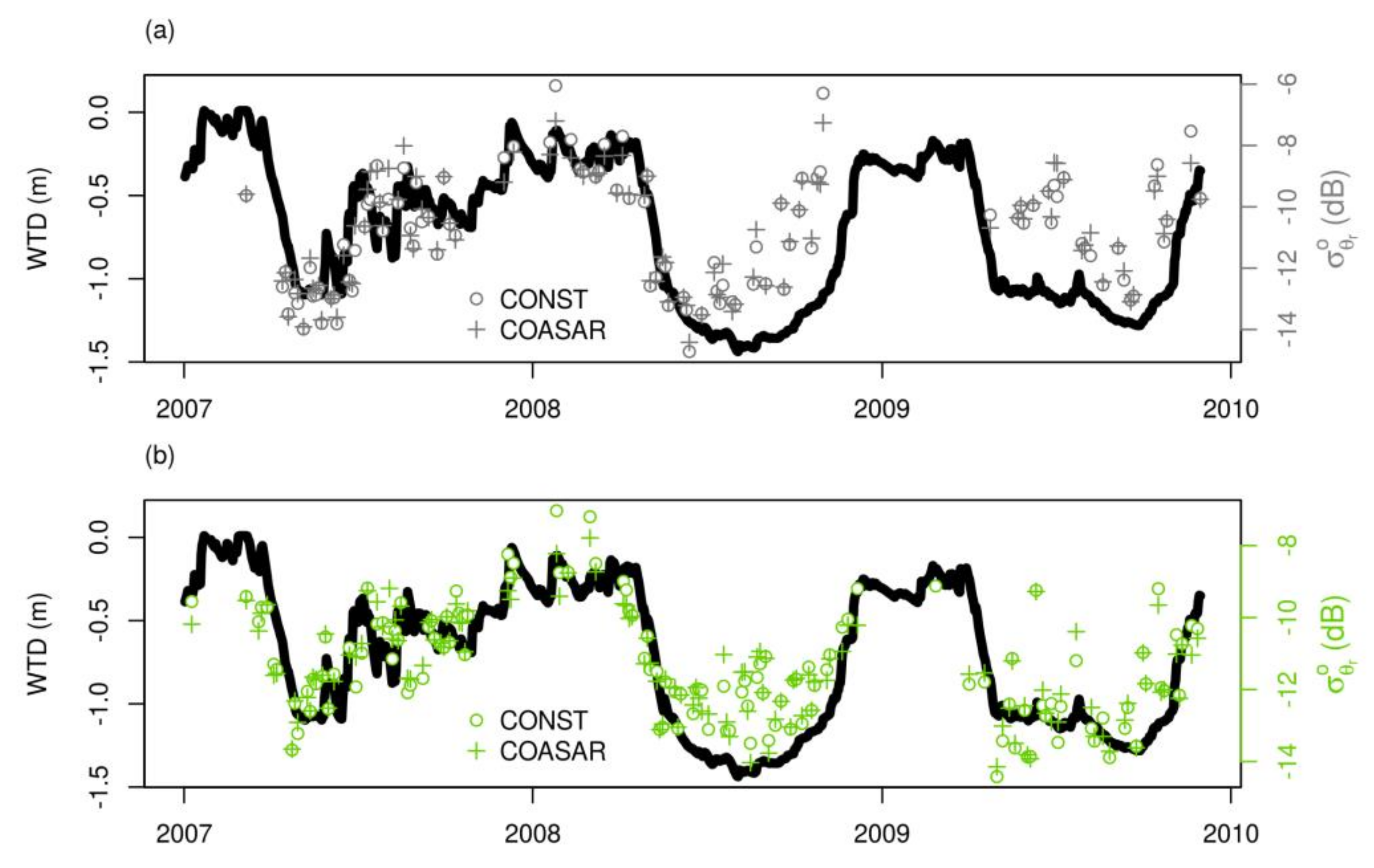
4.2. Comparison of Backscatter and Water Table Depth Time Series

For a first visual impression of the relation between backscatter and WTD, an example time series of a site (lat: 53.995°N, lon: 12.233°E, corresponding to site of Figure 4a) with an intermediate R value (des.: R = 0.5, asc.: R = 0.6) is given in Figure 5. The shown backscatter values were normalized to θ_r = 40° using site-specific constant slope correction (CONST) and cross-over angle concept normalization based on slope climatologies derived from ASAR data (COASAR). Time series of descending and ascending data are shown separately in Figure 5a,b, respectively, and the corresponding scatterplot for both nodes is given in Figure 6 for the CONST method. The two figures show a number of typical features that we observed for many sites:

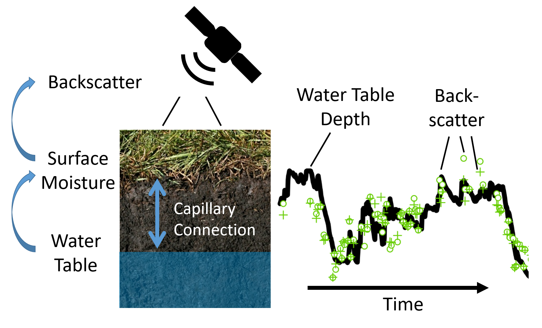
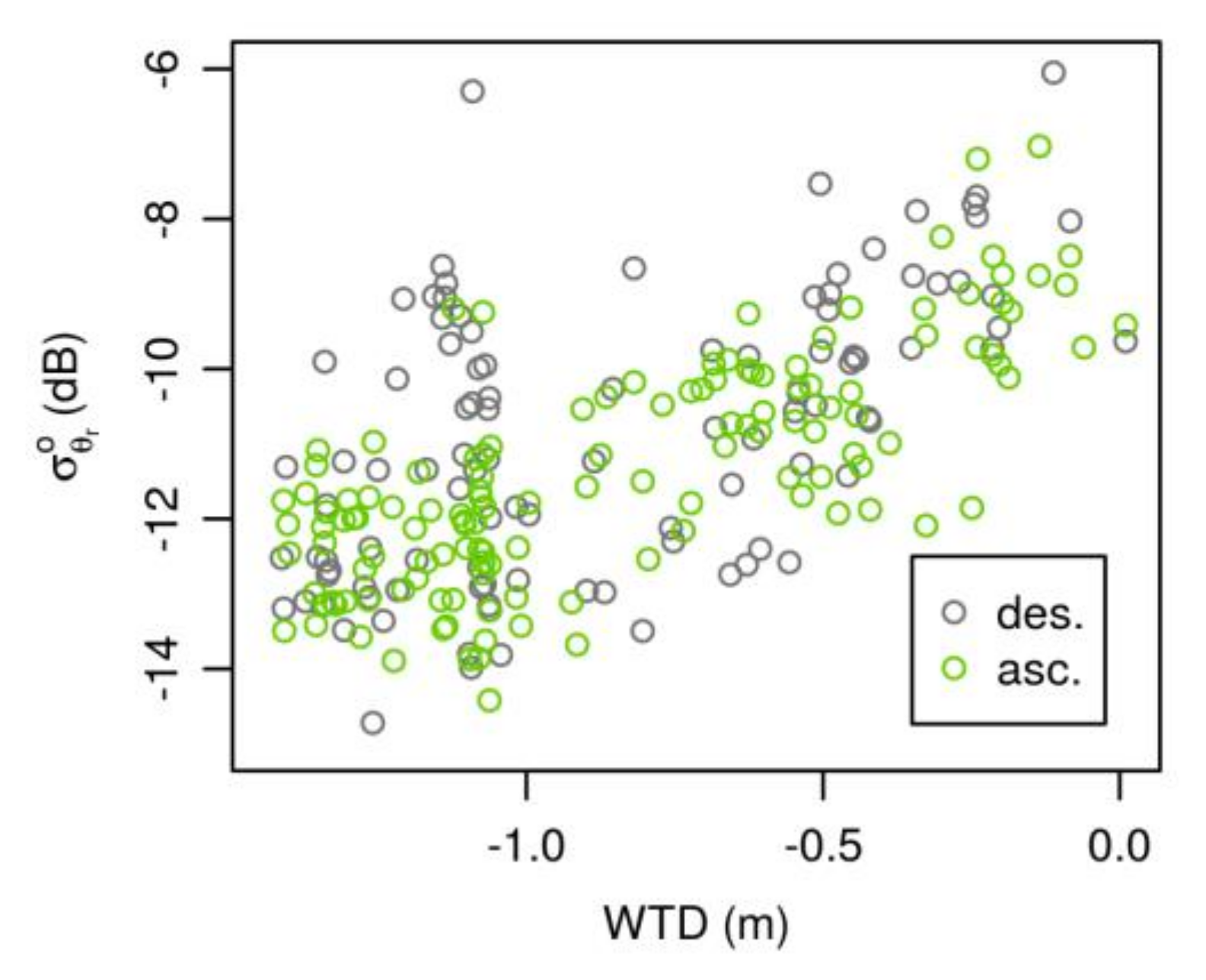
• There is a nearly linear increase of σ° with shallower water tables over most of the observed range of WTD, irrespective of the processing configuration (CONST, COASAR).
• The link between σ° and WTD becomes weaker towards the dry end of WTD. In Figure 6, the dependency seems to vanish at a WTD of approximately −1 m. We could not identify a systematic threshold WTD for all of our sites and, where present, it varied from about −0.5 to 1.5 m.
• The σ° time series enabled to monitor to some degree the interannual variability of WTD dynamics, i.e., anomalous dry or wet periods.
• The differences between descending and ascending σ° time series are remarkable during parts of the year, although not systematic over different sites.

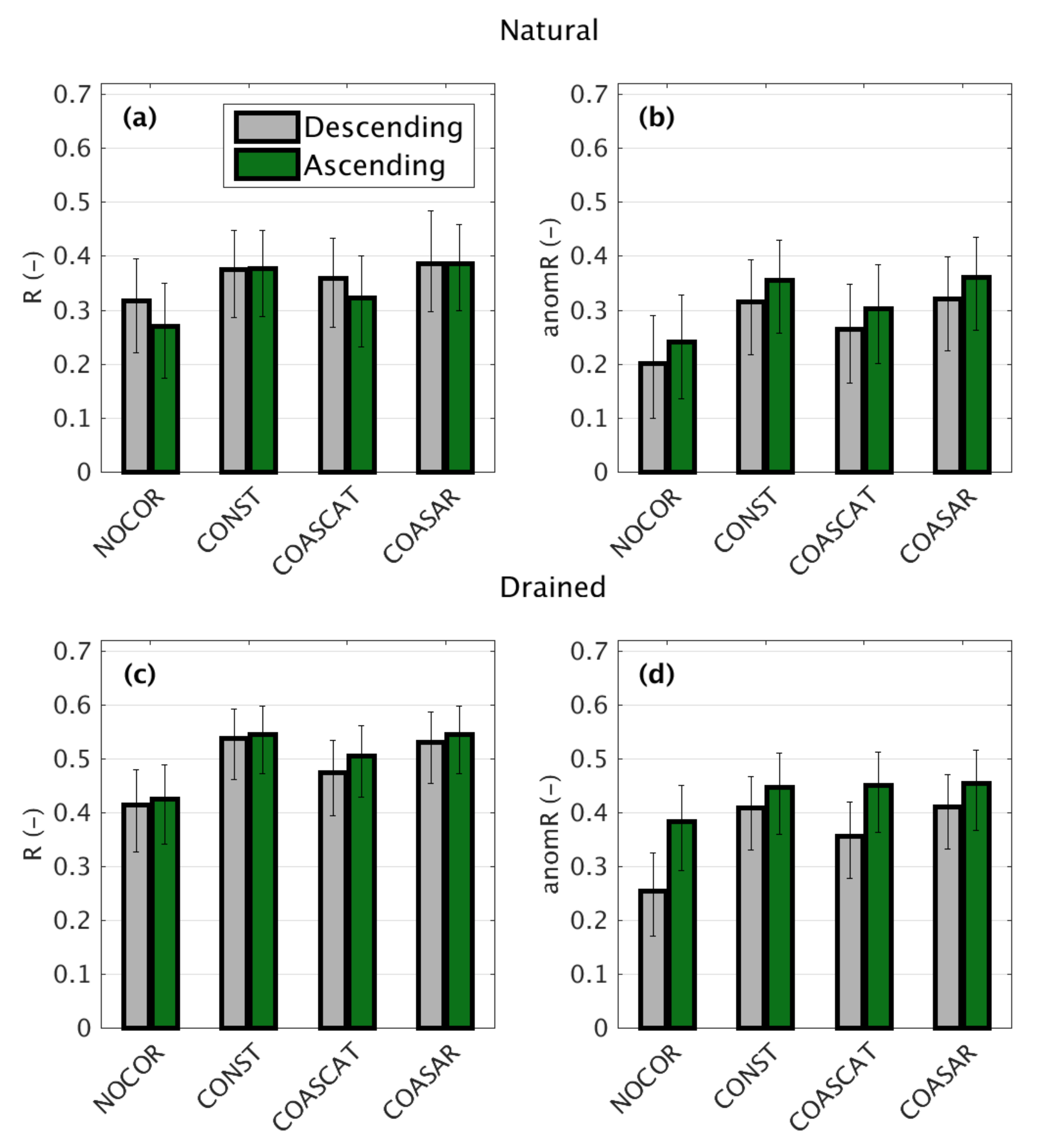
4.3. Skill Metrics for Different Backscatter Time Series

An overview of the skill metrics of the four different backscatter time series at all sites is shown in Figure 7 and

Table 1. Summary of skill metrics averaged across all sites and both orbital nodes.

Method	R ± ½ CI 1	anomR ± ½ CI
NOCOR	0.37 ± 0.04	0.27 ± 0.05
CONST	0.46 ± 0.04	0.38 ± 0.04
COASCAT	0.42 ± 0.04	0.34 ± 0.04
COASAR	0.47 ± 0.04	0.39 ± 0.04

¹ The 95% confidence interval (CI) is narrower than shown in Figure 7 due to further aggregation over natural and drained sites, and descending and ascending nodes.

. It can be observed that R and anomR are, regardless of the kind of incidence angle correction, considerably lower for natural (R = 0.38, anomR = 0.33) than for drained (R = 0.54, anomR = 0.43) peatland sites, with small differences for ascending and descending data. It is further shown that any incidence angle correction (significantly) improves correlation coefficients for both the original time series and anomaly time series with respect to using σ° without correction for the influence of local incidence angle. Small, but insignificant, differences can be observed among the different incidence angle corrections. CONST and COASAR appear to perform slightly better than COASCAT. CONST and COASAR show very similar skill metrics.

Figure 8 summarizes backscatter intensity (CONST) and correlation coefficient over all sites relative to the water table depth. The figure illustrates two major observations that we made:

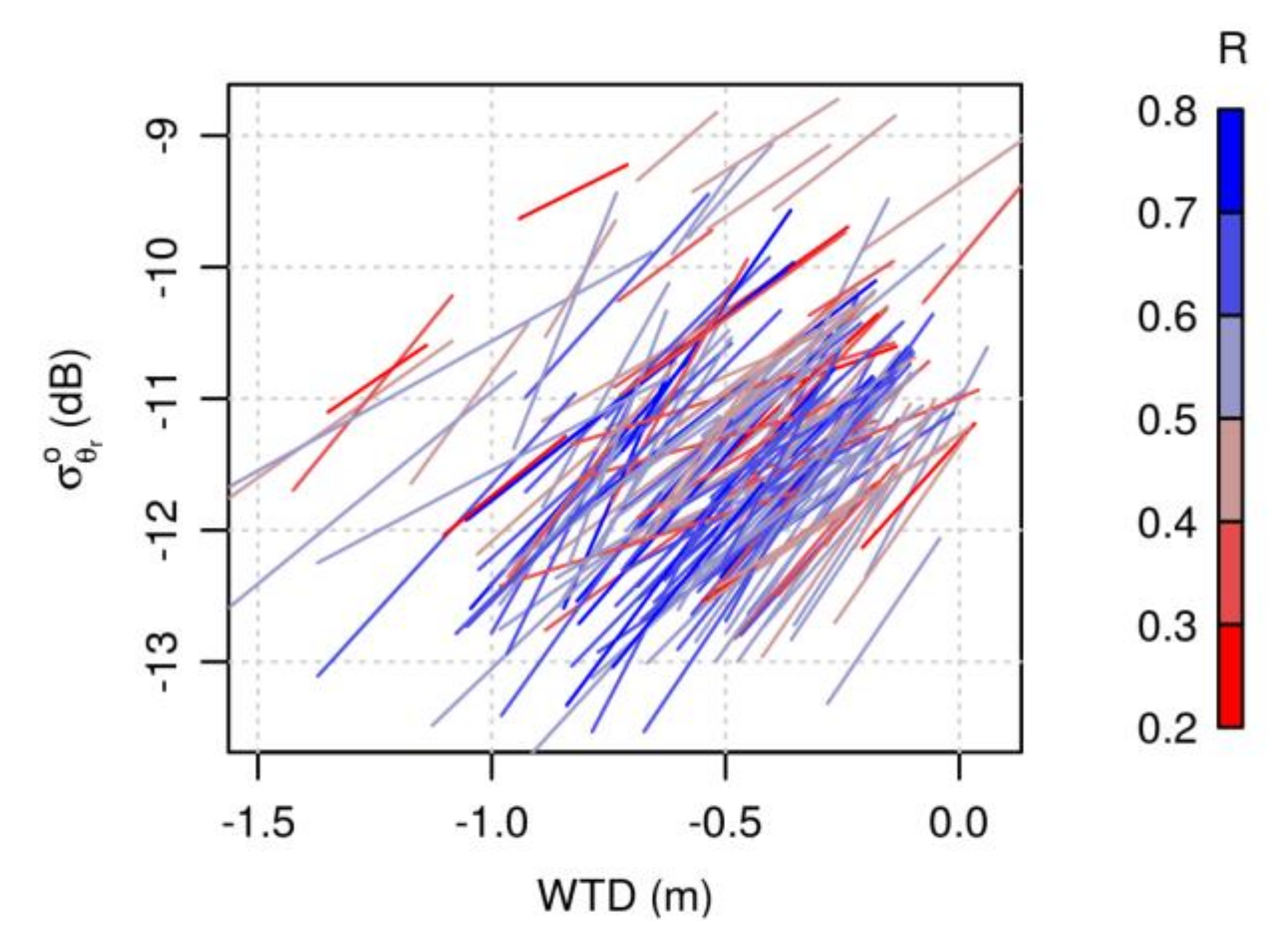
• The temporal correlation coefficient between σ° and WTD is rather independent of the mean WTD of a site. High R values of up to 0.8 can be observed for deeply-drained sites as well as for sites with shallow WTD (which comprise shallowly-drained, as well as natural sites).
• While at all sites a positive correlation can be observed, there is a strong variability of the absolute level of σ° across sites.

5. Discussion

5.1. Differences between Descending and Ascending Data

The correlation metrics quantifying the relationship between σ° and WTD differ for ascending and descending data subsets (Figure 7). Differences between σ° observations from different orbital nodes can be caused by, e.g., diurnal differences in the actual geophysical parameters, as well as anisotropic behavior of the land surface under different viewing geometries. The example time series of Figure 5 showed slightly higher σ° for descending (9 am local time) pass, which could be explained by shallower water tables in the morning in case of significant diurnal water table fluctuations [38], capillary equilibration of top soil moisture during night time or dew effects in morning hours. However, we could not observe that this is systematically the case for all of our sites. Azimuthal anisotropy, on the other hand, can be caused by corner reflectors, such as buildings, within the pixel, as well as the predominant orientation of rows of crops, such as maize or wheat [39]. Over a large number of different sites, this anisotropy typically disappears due to different orientations of corner reflectors and crop rows. On average, descending and ascending σ° values were not significantly different. However, the ascending node showed on average a higher anomaly correlation coefficient for both natural and drained peatlands (Figure 7b,d), for which we could not find a clear explanation.

5.2. Impact of Different Processing Configurations

CONST and COASAR resulted in better skill metrics than COASCAT (e.g., Table 1), which was not surprising, as we noticed considerable differences between ASCAT and ASAR seasonal slopes (Figure 4). ASCAT slopes were determined for a much coarser resolution and are apparently not representative for the peatland sites that are typically much smaller than the ASCAT grid spacing (here 12.5 km).

However, COASAR was not superior to CONST. Apparently, the concept of the cross-over angle vegetation correction could not show its strength on the basis of the ASAR derived site-specific slope time series. Frequent biomass drops due to grassland and cropland management are probably one important factor which cannot be reproduced with a climatology time series due to cut dates that differ from year to year. Figure 4c shows an example for which we know that it is a grassland area that is subject to frequent cuts (about four times per year). The regular reduction of biomass occurring at dates that vary from year to year probably contributes to the fact that the slope parameter is rather constant when pooling data from multiple years. Grassland cut dynamics could not be captured due to the limited amount of available data and the consequent need for large window sizes (on average 90 days).

Overall, the temporal standard deviation of the ASAR slopes was lower than the temporal standard deviation of the ASCAT slopes for 75% of the sites, and nearly constant (standard deviation <0.01 dB/degree) for 35% of the sites. The lower intra-annual slope variability reduced potential positive impacts of the cross-over angle concept.

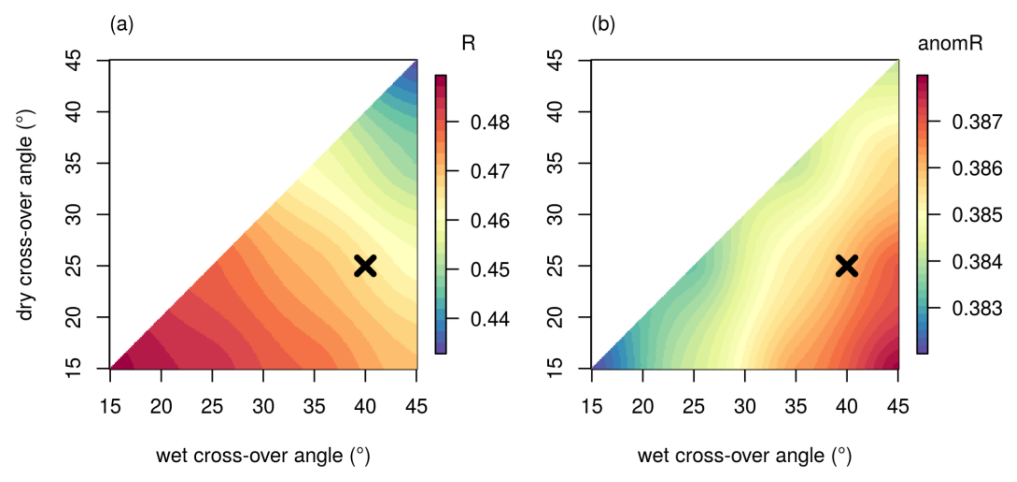
5.2.1. Possible Optimization of Cross-Over Angles over Peatlands

Applications of the cross-over angle concept typically use the dry and wet cross-over angles originally determined over the Iberian Peninsula by Wagner et al. [18] like we did here for COASCAT and COASAR. These angles might be suboptimal for an application over peatlands. Moisture contents are much higher in peat than in mineral soils and reach up to about 70–80 vol % in degraded and up to about 80–90 vol % in natural peatlands. Furthermore, the dry and wet reference states over peatlands are not comparable with dry and wet references in mineral soils. Moisture content at the wilting point, which is typically referred to as ‘dry reference’ in mineral soils [40], might often not be reached in the top few centimeters of peat soils when a capillary connection to the groundwater reservoir is present over the whole year. Moisture content at field capacity, which is typically referred to as the ‘wet reference’ in mineral soils, is lower than complete saturation occurring in peatlands when the WTD reaches the soil surface.

Furthermore, WTD time series have a strong seasonal pattern. Figure 9 shows the backscatter values from two 90 day windows covering the low and high slope periods of the example slope climatology from Figure 4a. The fitted slopes were steeper for winter than for summer. The strong seasonality of backscatter and water table depth may often be the cause that the dry reference is only reached in summer and the wet reference only reached in winter. These two references are indicated as solid lines. In contrast, the dry reference is basically never observed in winter and the wet reference never in summer. To demonstrate the issue, we indicate the hypothetical dry and wet references, in winter and summer, respectively, as dashed lines. They are drawn with an offset below and above each of the corresponding point clouds indicating that they are not reached. Figure 9 illustrates that it would not be possible to derive the θ_d and θ_w directly from data analysis.

To evaluate whether typical peatland cross-over angles could be determined by parameter optimization, we created COASAR backscatter datasets using the dynamic ASAR-based β_doy together with a range of cross-angle combinations. For each pair of cross-angles, we evaluated the temporal skill metrics averaged across all drained and natural sites, and across both ascending and descending node. The pairs of cross-angles compose a grid of dry and wet cross-over angles from 15° to 45°, covering the range for which we determined the slope and assumed linearity. Under the assumption that the total backscatter amplitude due to changing moisture is smaller for states with high aboveground biomass than for states with low aboveground biomass [18], θ_d must be smaller than θ_w and the grid of cross-angle pairs is limited accordingly.

Figure 10 shows the resulting skill metrics R and anomR. The two figures indicate optimal cross-over angles for different combinations of θ_d and θ_w. Whereas R improves with decreasing θ_d and θ_w, anomR shows higher values with increasing θ_w, but the anomR values are far less dependent on the cross-over angles than R. It is not possible to find a well-defined optimum for both metrics. A trade-off between optima of both metrics indicates optimal cross-over angles somewhere at θ_d = 15° and θ_w = 30°. It is however very questionable to suggest these angles as being more appropriate than the default angles. The fact that optimal angles for R would be in the range of negative angles (tested, not shown) indicates a general difficulty of the optimization of cross-over angles based on skill metrics. 66% of our slope climatologies showed a seasonal pattern that is negatively correlated with the seasonal pattern of the water table depth dynamics. We noticed, especially for sites with low R values, that R can be considerably improved by very low cross-over angles when the slope climatology showed this seasonal pattern. Low cross-over angles increase the influence of the vegetation dynamics on backscatter (see Figure 2). When the backscatter values themselves showed little correlation with WTD, the seasonal pattern of the slope climatology itself becomes a major predictor for WTD for low cross-over angles, which obviously results in spurious correlation. Backscatter time series from cross-over angles that were much smaller than 15° (not shown) were strongly smoothed with little remaining interannual variability due to the high impact of the invariant slope climatology. As a consequence, anomaly information gets lost which is, by its trend and averaged over all sites, seen in the pattern of anomR (Figure 10b).

5.3. Potential and Limitations of C-Band Backscatter for Water Table Depth Monitoring

Our results indicate that C-band backscatter data contains information that is useful for the monitoring of below-ground water level fluctuations in peatlands. In the example shown in Figure 6, the dependency between σ° and WTD seems to vanish at a WTD of approximately −1 m. We could not identify similar thresholds for which the dependency gets weaker for all of our sites, and where present, the value varied from about −0.5 to −1.5 m. The value can be interpreted as the threshold at which a strong capillary connection between WTD and topsoil moisture gets lost. Another possible explanation is offered by the fact that deep water tables predominantly occur during the summer months (Figure 5) when the vegetation canopy is typically well developed and considerable volume scattering and/or attenuation may take place. As a result, the backscatter signal may become decoupled from soil water dynamics.

Our evaluation is limited to the local temporal dynamics (i.e., excluding spatial patterns) and relying on the change detection approach, like common soil moisture products from C-band backscatter [20]. Soil moisture time series from C-band backscatter are typically location-specific ‘wetness’ time series scaled to the range between field capacity and wilting point moisture estimates from soil texture maps and pedotransfer functions. Figure 8 indicates that without knowledge about additional factors that influence backscatter intensity (e.g., surface roughness, vegetation, static open water bodies) C-band backscatter cannot be used to map the absolute WTD in space.

Across all peatlands, correlation coefficients between σ° and WTD were on average 0.46 and 0.38 (CONST correction) for original and anomaly time series, respectively (Table 1), and as high as typical values reported for the correlation between ASCAT SM retrievals and in situ observed top soil moisture over mineral soils [20]. Like soil moisture data, ground-based WTD data represent point measurements. However, water levels are changing more synchronously in space than top soil moisture dynamics in mineral soils, which may increase representativeness of WTD measurements for homogeneous footprints. However, in managed peatlands, WTD and its dynamics can change abruptly from field to field due to different land use and water management [21] and σ° might capture some adjacent mineral soils as well (up to 30%, see Section 2.2), i.e., footprint-scale correlations between σ° and WTD are probably higher than indicated in our study here which included heterogeneous local effects. Finer resolution data and an improved radiometric accuracy of Sentinel-1 will probably reduce this effect and improve the skill metrics. At 25% of all sites R and anomR of >0.6 and >0.5, respectively, could be achieved, indicating that the potential of C-band backscatter may increase with finer resolution in future. Furthermore, the use of VV polarization was unfavorable compared to the non-available HH polarization [11]. Potential future missions that include HH data might further reduce the uncorrected part of the confounding effects of the vegetation layer.

As mentioned earlier, it was observed that R and anomR are, regardless of the kind of incidence angle correction, considerably lower for the natural than for drained peatland sites. Specular reflection due to significant amounts of free water surfaces during high water levels has been mentioned above as a reason for lowering σ° during very wet periods. However, in the site-specific scatterplots that underlie Figure 8, we could observe lower σ° values for shallower WTD for only a few sites and a very limited amount of data points, i.e., amounts of inundated areas were probably relatively small and of short duration for our peatlands sites. The test-wise manual elimination of these data points did show only very little improvement for R and anomR over the natural peatlands. Additionally, the use of Spearman instead of Pearson correlation to possibly account for a decreasing linear dependency for high water levels did not show any improvement.

In addition to inundation, other differences between natural and drained peatlands may additionally cause the difference in skill metrics. Drained peatlands are used for agriculture, have more compact soils, which causes them to behave somewhat more like mineral soils. In contrast, natural peatlands are often characterized by a considerable microrelief commonly referred to as ‘hummock and hollow’ microrelief which can include soil elevation changes of approximately 20 to 40 cm over one or two meter [41]. Additionally, a ground surface is poorly defined for natural peatlands with weakly decomposed, ‘fluffy’ peat soils and the ‘interface’ between vegetation and peat is transitional over several centimeters. Regarding the low penetration depth of C-band backscatter of only one or two centimeters, both characteristics of natural peatlands may cause scattering mechanisms and incidence angle dependencies to be more complex, e.g., moisture-dependent, which may weaken the correlation between backscatter and water table depth.

It is promising that our data set showed high correlation coefficients for the anomaly time series. In order to mitigate greenhouse gas emissions and subsidence, measures are undertaken to both restore the natural hydrological dynamics and avoid anomalously strong drops of water table depth during drier summers, e.g., by re-wetting or, more recently, also by means of subsurface irrigation of agricultural sites [42]. Such anomalous WTD drops could be effectively evaluated over large areas with σ° anomaly time series. Furthermore, the anomalies could help to distinguish between climate effects and insufficient water management of restored sites. Peat oxidation mainly occurs during summer when temperatures are high and water tables are deep. For mitigation measures, it is thus crucial to keep the water table depth as close as possible to the shallow target level of the water management plan during the summer period.

6. Conclusions

In this study, we evaluated the relationship between ENVISAT Advanced Synthetic Aperture Radar (ASAR) C-band backscatter (σ°) time series and in situ observed WTD dynamics over 17 peatlands in Germany covering deeply-drained to natural conditions, excluding peatlands dominated by forest or inundation periods. The results showed increasing σ° with shallower WTD (=wetter conditions), with average temporal Pearson correlation coefficients of 0.38 and 0.54 (-) for natural (also including disturbed and rewetted/restored states) and agriculturally-used drained peatlands, respectively. The anomaly correlation further highlighted the potential of ASAR backscatter to capture interannual variations with values of 0.33 and 0.43 (-), for natural and drained peatlands.

Based on our evaluation using extensive data from both natural and drained dominated footprints peatlands we conclude that:

• backscatter is a good indicator for water table depth dynamics, but the interpretation seems to be more difficult for natural than for drained peatlands;
• the use of ENVISAT-ASAR (fine resolution) as opposed to ASCAT (coarse) has a high potential for future analysis over peatlands; and
• the use of various incidence angle correction techniques improved the correlation between backscatter and water table depth but differences between the various methods were small.

We believe that the strong capillary link between water table depth and topsoil moisture in peatlands is the main explanation for the good correlation between the C-band satellite signal, which is sensitive to soil moisture variation in the top one or two centimeters, and WTD observations, which are several centimeters to more than one meter below ground.

The increasing availability of Sentinel-1 C-band data may enhance the applicability for WTD monitoring over peatlands for several reasons. The new generation of SAR technology provides data with higher radiometric accuracy, and finer spatial and temporal resolution. The additional availability of VH polarization images at the same time as VV polarization images and their different sensitivity to vegetation changes might allow identification of grassland cut events [43]. This will allow new opportunities to correct for vegetation dynamics with the cross-over angle concept which was not possible in our study with ENVISAT-ASAR data.

Our study took advantage of a recently compiled dataset for a range of German peatlands. Yet, these peatlands are not necessarily representative of all peatlands across the globe. The extensive natural peatlands over Siberia and Canada are not comparable with the natural peatlands in our dataset as they often include much more open water surfaces, not only static but also dynamic [15]. Already for our dataset, lower correlations were observed for natural peatlands; for peatlands with more open water (both as larger ponds and partial inundation the in meter-scale microtopography) a simple correlation between σ° and WTD will probably perform worse and specific methods need to be further developed that deal with partial inundation [11].

References

1. Tubiello, F.N.; Biancalani, R.; Salvatore, M.; Rossi, S.; Conchedda, G. A worldwide assessment of greenhouse gas emissions from drained organic soils. Sustainability 2016, 8. [Google Scholar] [CrossRef]
2. Kieckbusch, J.J.; Schrautzer, J. Nitrogen and phosphorus dynamics of a re-wetted shallow-flooded peatland. Sci. Total Environ. 2007, 380, 3–12. [Google Scholar] [CrossRef] [PubMed]
3. Grayson, R.; Holden, J.; Rose, R. Long-term change in storm hydrographs in response to peatland vegetation change. J. Hydrol. 2010, 389, 336–343. [Google Scholar] [CrossRef]
4. Chapman, S.; Buttler, A.; Francez, A.J.; Laggoun-Défarge, F.; Vasander, H.; Schloter, M.; Combe, J.; Grosvernier, P.; Harms, H.; Epron, D.; et al. Exploitation of northern peatlands and biodiversity maintenance: A conflict between economy and ecology. Front. Ecol. Environ. 2003, 1, 525–532. [Google Scholar] [CrossRef]
5. Joosten, H. The Global Peatland CO2 Picture. Peatland Status and Drainage Related Emissions in All Countries of The World; Wetlands International: Wageningen, The Netherlands, 2010; p. 36. [Google Scholar]
6. Tiemeyer, B.; Bechtold, M.; Belting, S.; Freibauer, A.; Förster, C.; Schubert, E.; Dettmann, U.; Frank, S.; Fuchs, D.; Gelbrecht, J.; et al. Moorschutz in Deutschland—Optimierung des Moormanagements in Hinblick auf den Schutz der Biodiversität und der Ökosystemleistungen. BfN Skripten 2017, 462, 320. [Google Scholar]
7. Bircher, S.; Andreasen, M.; Vuollet, J.; Vehviläinen, J.; Rautiainen, K.; Jonard, F.; Weihermüller, L.; Zakharova, E.; Wigneron, J.P.; Kerr, H.Y. Soil moisture sensor calibration for organic soil surface layers. Geosci. Instrum. Methods Data Syst. 2016, 5, 109–125. [Google Scholar] [CrossRef]
8. Kasischke, E.S.; Bourgeau-Chavez, L.L.; Rober, A.R.; Wyatt, K.H.; Waddington, J.M.; Turetsky, M.R. Effects of soil moisture and water depth on ERS SAR backscatter measurements from an Alaskan wetland complex. Remote Sens. Environ. 2009, 113, 1868–1873. [Google Scholar] [CrossRef]
9. Harris, A.; Bryant, R.G. A multi-scale remote sensing approach for monitoring northern peatland hydrology: Present possibilities and future challenges. J. Environ. Manag. 2009, 90, 2178–2188. [Google Scholar] [CrossRef] [PubMed]
10. Meingast, K.M.; Falkowski, M.J.; Kane, E.S.; Potvin, L.R.; Benscoter, B.W.; Smith, A.M.S.; Bourgeau-Chavez, L.L.; Miller, M.E. Spectral detection of near-surface moisture content and water-table position in northern peatland ecosystems. Remote Sens. Environ. 2014, 152, 536–546. [Google Scholar] [CrossRef]
11. Kim, J.W.; Lu, Z.; Gutenberg, L.; Zhu, Z. Characterizing hydrologic changes of the Great Dismal Swamp using SAR/InSAR. Remote Sens. Environ. 2017, 198, 187–202. [Google Scholar] [CrossRef]
12. Tiemeyer, B.; Albiac Borraz, E.; Augustin, J.; Bechtold, M.; Beetz, S.; Beyer, C.; Drösler, M.; Ebli, M.; Eickenscheidt, T.; Fiedler, S.; Förster, C.; Freibauer, A.; et al. High emissions of greenhouse gases from grasslands on peat and other organic soils. Glob. Chang. Biol. 2016, 22, 4134–4149. [Google Scholar] [CrossRef] [PubMed]
13. Kasischke, E.S.; Smith, K.B.; Bourgeau-Chavez, L.L.; Romanowicz, E.A.; Brunzell, S.; Richardson, C.J. Effects of seasonal hydrologic patterns in south Florida wetlands on radar backscatter measured from ERS-2 SAR imagery. Remote Sens. Environ. 2003, 88, 423–441. [Google Scholar] [CrossRef]
14. Kim, J.W.; Lu, Z.; Lee, H.; Shum, C.K.; Swarzenski, C.M.; Doyle, T.W.; Baek, S.H. Integrated analysis of PALSAR/Radarsat-1 InSAR and ENVISAT altimeter data for mapping of absolute water level changes in Louisiana wetlands. Remote Sens. Environ. 2009, 113, 2356–2365. [Google Scholar] [CrossRef]
15. Bartsch, A.; Trofaier, A.M.; Hayman, G.; Sabel, D.; Schlaffer, S.; Clark, D.B.; Blyth, E. Detection of open water dynamics with ENVISAT ASAR in support of land surface modelling at high latitudes. Biogeosciences 2012, 9, 703–714. [Google Scholar] [CrossRef] [Green Version]
16. Schlaffer, S.; Chini, M.; Dettmering, D.; Wagner, W. Mapping wetlands in Zambia using seasonal backscatter signatures derived from ENVISAT ASAR time series. Remote Sens. 2016, 8. [Google Scholar] [CrossRef]
17. Ulaby, F.T.; Moore, R.K.; Fung, A.K. Microwave Remote Sensing: Active and Passive. Volume 3—From Theory to Applications; Artech House, Inc.: Norwood, MA, USA, 1986; Volume 3, ISBN 0890061920. [Google Scholar]
18. Wagner, W.; Lemoine, G.; Borgeaud, M.; Rott, H. A study of vegetation cover effects on ers scatterometer data. IEEE Trans. Geosci. Remote Sens. 1999, 37, 938–948. [Google Scholar] [CrossRef]
19. Dorigo, W.; Wagner, W.; Albergel, C.; Albrecht, F.; Balsamo, G.; Brocca, L.; Chung, D.; Ertl, M.; Forkel, M.; Gruber, A.; et al. ESA CCI Soil Moisture for improved Earth system understanding: State-of-the art and future directions. Remote Sens. Environ. 2017, 203, 185–215. [Google Scholar] [CrossRef]
20. Dorigo, W.A.; Gruber, A.; De Jeu, R.A.M.; Wagner, W.; Stacke, T.; Loew, A.; Albergel, C.; Brocca, L.; Chung, D.; Parinussa, R.M.; et al. Evaluation of the ESA CCI soil moisture product using ground-based observations. Remote Sens. Environ. 2015, 162, 380–395. [Google Scholar] [CrossRef]
21. Bechtold, M.; Tiemeyer, B.; Laggner, A.; Leppelt, T.; Frahm, E.; Belting, S. Large-scale regionalization of water table depth in peatlands optimized for greenhouse gas emission upscaling. Hydrol. Earth Syst. Sci. 2014, 18, 3319–3339. [Google Scholar] [CrossRef]
22. Pathe, C.; Wagner, W.; Sabel, D.; Doubkova, M.; Basara, J.B. Using ENVISAT ASAR global mode data for surface soil moisture retrieval over Oklahoma, USA. IEEE Trans. Geosci. Remote Sens. 2009, 47, 468–480. [Google Scholar] [CrossRef]
23. Ikonen, J.; Smolander, T.; Pratola, C. ESA Climate Change Initiative Phase II Soil Moisture. Comprehensive Error Characterisation Report Revision 1 (CECR) D2.2.1. Verion 1.0.; ESA: Paris, France, 2016. [Google Scholar]
24. European Space Agency (ESA). ENVISAT-1 Products Specifications Volume 9: DORIS Product Specifications; Document reference: PO-RS-MDA-GS-2009; ESA: Paris, France, 2008. [Google Scholar]
25. Gruber, A.; Wagner, W.; Hegyiova, A.; Greifeneder, F.; Schlaffer, S. Potential of Sentinel-1 for high-resolution soil moisture monitoring. In International Geoscience and Remote Sensing Symposium (IGARSS); ESA: Paris, France, 2013; pp. 4030–4033. [Google Scholar]
26. Torres, R.; Snoeij, P.; Geudtner, D.; Bibby, D.; Davidson, M.; Attema, E.; Potin, P.; Rommen, B.Ö.; Floury, N.; Brown, M.; et al. GMES Sentinel-1 mission. Remote Sens. Environ. 2012, 120, 9–24. [Google Scholar] [CrossRef]
27. Small, D.; Schubert, A. Guide to ASAR Geocoding; ESA-ESRIN Technical Note RSL-ASAR-GC-AD, Iss. 1.01; University of Zurich: Zurich, Switzerland, 2008; p. 36. [Google Scholar]
28. Jarvis, A.; Reuter, H.; Nelson, A.; Guevara, E. Hole-filled Seamless SRTM Data V4. International Centre for Tropical Agriculture (CIAT), 2008.
29. Gevaert, A.I.; Parinussa, R.M.; Renzullo, L.J.; van Dijk, A.I.J.M.; de Jeu, R.A.M. Spatio-temporal evaluation of resolution enhancement for passive microwave soil moisture and vegetation optical depth. Int. J. Appl. Earth Obs. Geoinfom. 2015, 45, 235–244. [Google Scholar] [CrossRef]
30. IPCC. IPCC Guidelines For National Greenhouse Gas Inventories; Eggleston, H.S., Buendia, L., Miwa, K., Ngara, T.K.T., Eds.; IGES: Yokohama, Japan, 2006. [Google Scholar]
31. Von Asmuth, J.R.; Maas, K.; Bakker, M.; Petersen, J. Modeling time series of ground water head fluctuations subjected to multiple stresses. Ground Water 2008, 46, 30–40. [Google Scholar] [CrossRef] [PubMed]
32. Loew, A.; Ludwig, R.; Mauser, W. Derivation of surface soil moisture from ENVISAT ASAR wide swath and image mode data in agricultural areas. IEEE Trans. Geosci. Remote Sens. 2006, 44, 889–898. [Google Scholar] [CrossRef]
33. Hahn, S.; Reimer, C.; Vreugdenhil, M.; Melzer, T.; Wagner, W. Dynamic Characterization of the Incidence Angle Dependence of Backscatter Using Metop ASCAT. IEEE J. Sel. Top. Appl. Earth Obs. Remote Sens. 2017, 10, 2348–2359. [Google Scholar] [CrossRef]
34. Van Doninck, J.; Wagner, W.; Melzer, T.; De Baets, B.; Verhoest, N.E.C. Seasonality in the angular dependence of ASAR wide swath backscatter. IEEE Geosci. Remote Sens. Lett. 2014, 11, 1423–1427. [Google Scholar] [CrossRef]
35. R Core Team. R Development Core Team. Available online: http://www.r-project.org/ (accessed on 11 November 2018).
36. Bates, D.; Maechler, M.; Bolker, B.; Walker, S. Fitting Linear Mixed-Effects Models using lme4. J. Stat. Softw. 2015, 67, 1–48. [Google Scholar] [CrossRef]
37. De Lannoy, G.J.M.; Reichle, R.H. Global Assimilation of Multiangle and Multipolarization SMOS Brightness Temperature Observations into the GEOS-5 Catchment Land Surface Model for Soil Moisture Estimation. J. Hydrometeorol. 2016, 17, 669–691. [Google Scholar] [CrossRef]
38. Wang, P.; Pozdniakov, S.P. A statistical approach to estimating evapotranspiration from diurnal groundwater level fluctuations. Water Resour. Res. 2014, 50, 2276–2292. [Google Scholar] [CrossRef]
39. Bartalis, Z.; Scipal, K.; Wagner, W. Azimuthal anisotropy of scatterometer measurements over land. IEEE Trans. Geosci. Remote Sens. 2006, 44, 2083–2092. [Google Scholar] [CrossRef]
40. Wagner, W. Evaluation of the agreement between the first global remotely sensed soil moisture data with model and precipitation data. J. Geophys. Res. 2003, 108, 4611. [Google Scholar] [CrossRef]
41. Dettmann, U.; Bechtold, M. Deriving Effective Soil Water Retention Characteristics from Shallow Water Table Fluctuations in Peatlands. Vadose Zone J. 2016, 15. [Google Scholar] [CrossRef]
42. Querner, E.P.; Jansen, P.C.; van den Akker, J.J.H.; Kwakernaak, C. Analysing water level strategies to reduce soil subsidence in Dutch peat meadows. J. Hydrol. 2012, 446–447, 59–69. [Google Scholar] [CrossRef]
43. Ali, I.; Schuster, C.; Zebisch, M.; Förster, M.; Kleinschmit, B.; Notarnicola, C. First results of monitoring nature conservation sites in alpine region by using very high resolution (VHR) X-band SAR data. IEEE J. Sel. Top. Appl. Earth Obs. Remote Sens. 2013, 6, 2265–2274. [Google Scholar] [CrossRef]
Figure 1. Illustration of the potential link between the remote sensing signal, here backscatter coefficient (σ°), and below-ground water table depth (WTD) via a ‘capillary bridge’, i.e., the capillary-connected top soil and vegetation moisture in shallow water table depth environments.
Remotesensing 10 00536 g001
Figure 2. Illustration of the dependency of backscatter coefficients (σ°) to incidence angles (θ) with changing aboveground biomass. The slope and curvature are insensitive to soil moisture changes. At the cross-over angles (here indicated for a dry and a wet reference state, θd and θw, respectively), σ° is proposed to be rather independent of vegetation changes [18].
Remotesensing 10 00536 g002
Figure 3. Locations of 179 peatland WTD reference sites across Germany, representing a subset of Bechtold et al. [21]. The base map (geological map 1:200,000, BGR) shows the distribution of peatlands.
Remotesensing 10 00536 g003
Figure 4. Climatology time series examples of (a,c) slope and (b,d) curvature for two locations (a,b, lat: 53.995°N, lon: 12.233°E; c and d, lat: 53.694°N, lon: 8.822°E). Both footprints were dominated by grassland, but also included contributions from various other land covers. Curvature was not estimated for ASAR and set to 0.
Remotesensing 10 00536 g004
Figure 5. Example time series (lat: 53.995°N, lon: 12.233°E) of a drained peatland location with intermediate temporal correlation statistics showing monitored water table depth (WTD) and backscatter σ θ r dynamics for (a) descending, and (b) ascending, pass after constant slope incidence angle normalization (CONST) and cross-over angle concept normalization based on slope climatologies derived from ASAR data (COASAR).
Remotesensing 10 00536 g005
Figure 6. Corresponding scatterplot of data shown in Figure 5, indicating the observed correlation between water table depth (WTD) and backscatter σ θ r after constant slope incidence angle normalization (CONST) for descending and ascending nodes.
Remotesensing 10 00536 g006
Figure 7. Temporal Pearson correlation coefficient and 95% confidence intervals for original (R) and anomaly time series (anomR) for the differently processed backscatter time series (NOCOR: no incidence angle correction, CONST: constant slope normalization, COASCAT: cross-over angle concept using ASCAT slope and curvature climatology, COASAR: cross-over angle concept using slope climatology derived from ASAR data). Skills are shown for (a,b) natural, and (c,d) drained sites, both for descending and ascending nodes.
Remotesensing 10 00536 g007
Figure 8. Lines show the site-specific linear fits to backscatter (ascending data corrected using CONST method) and water table depth data for all peatland sites. Lines are colored by the temporal correlation coefficient (R) and drawn only for the inner 50% of the site-specific observed water table range for better readability.
Remotesensing 10 00536 g008
Figure 9. Backscatter σ° from two 90-day windows covering the low and high slope periods of the example site and slope climatology from Figure 4a. Black solid line: wet reference; red solid line: dry reference; black dashed line: hypothetical (not-observed) dry reference in winter; red dashed line: hypothetical (not-observed) wet reference in summer.
Remotesensing 10 00536 g009
Figure 10. Average time series (a) R and (b) anomR between observed WTD and backscatter estimates using various combinations of dry and wet cross-over angles. The metrics are averaged across all sites, ascending and descending node. The cross symbol indicates the commonly applied cross-over angles θd = 25° and θw = 40° at which R = 0.47 and anomR = 0.39 (see Table 1).
Remotesensing 10 00536 g010