Airborne Hyperspectral Evaluation of Maximum Gross Photosynthesis, Gravimetric Water Content, and CO2 Uptake Efficiency of the Mer Bleue Ombrotrophic Peatland

 , ,
, , 
Abstract
:
1. Introduction
2. Materials and Methods
2.1. Study Area
2.2. Airborne Hyperspectral Imagery (HSI)
2.3. Hyperspectral Imagery Pre-Processing
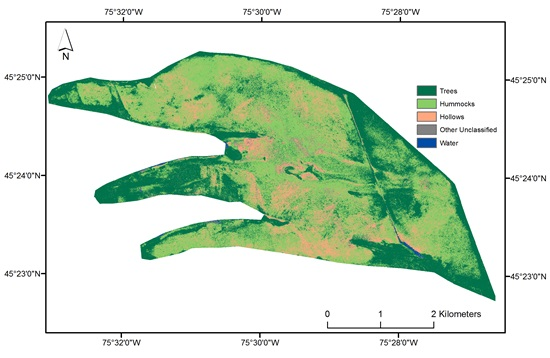
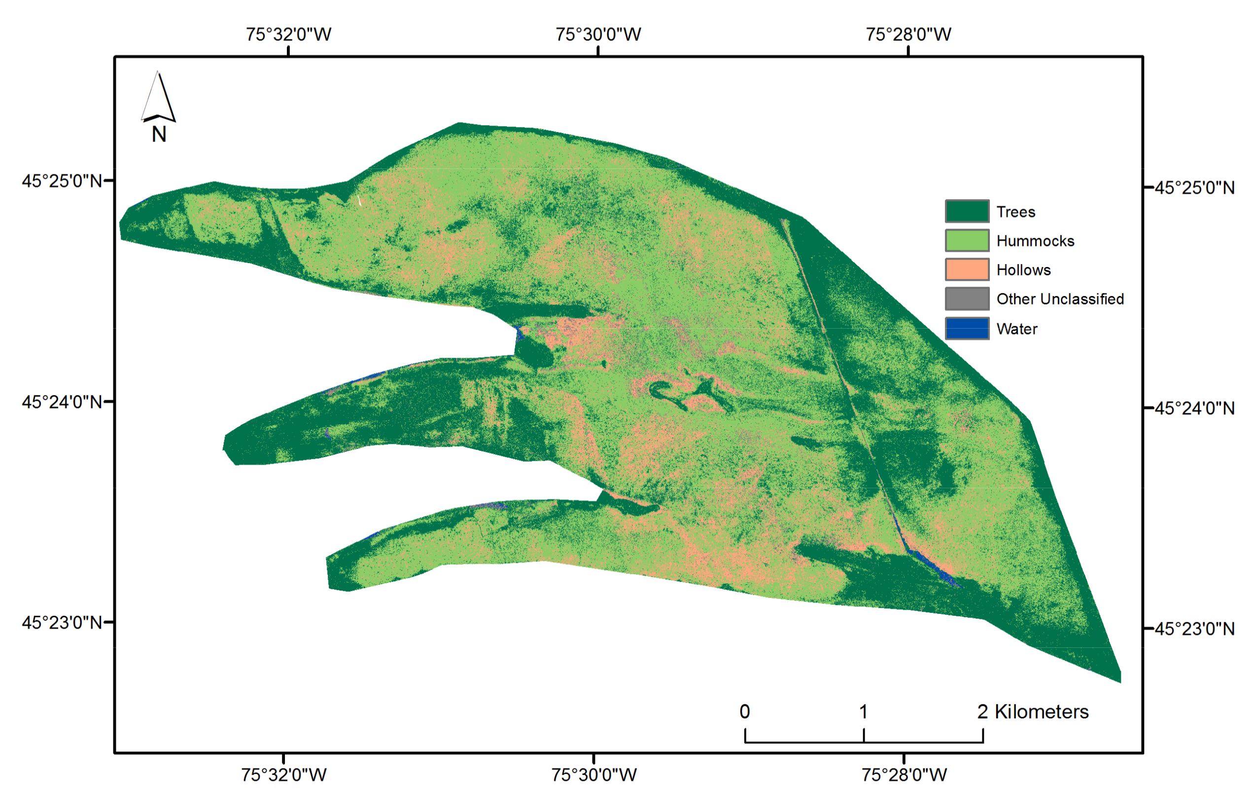
2.4. Hummock and Hollow Classification
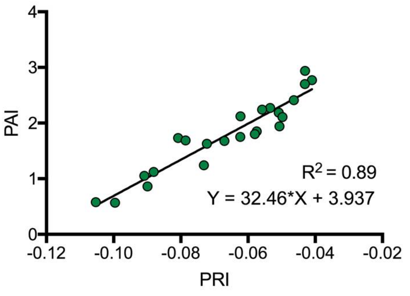
2.4.1. Plant Area Index In Situ Empirical Model
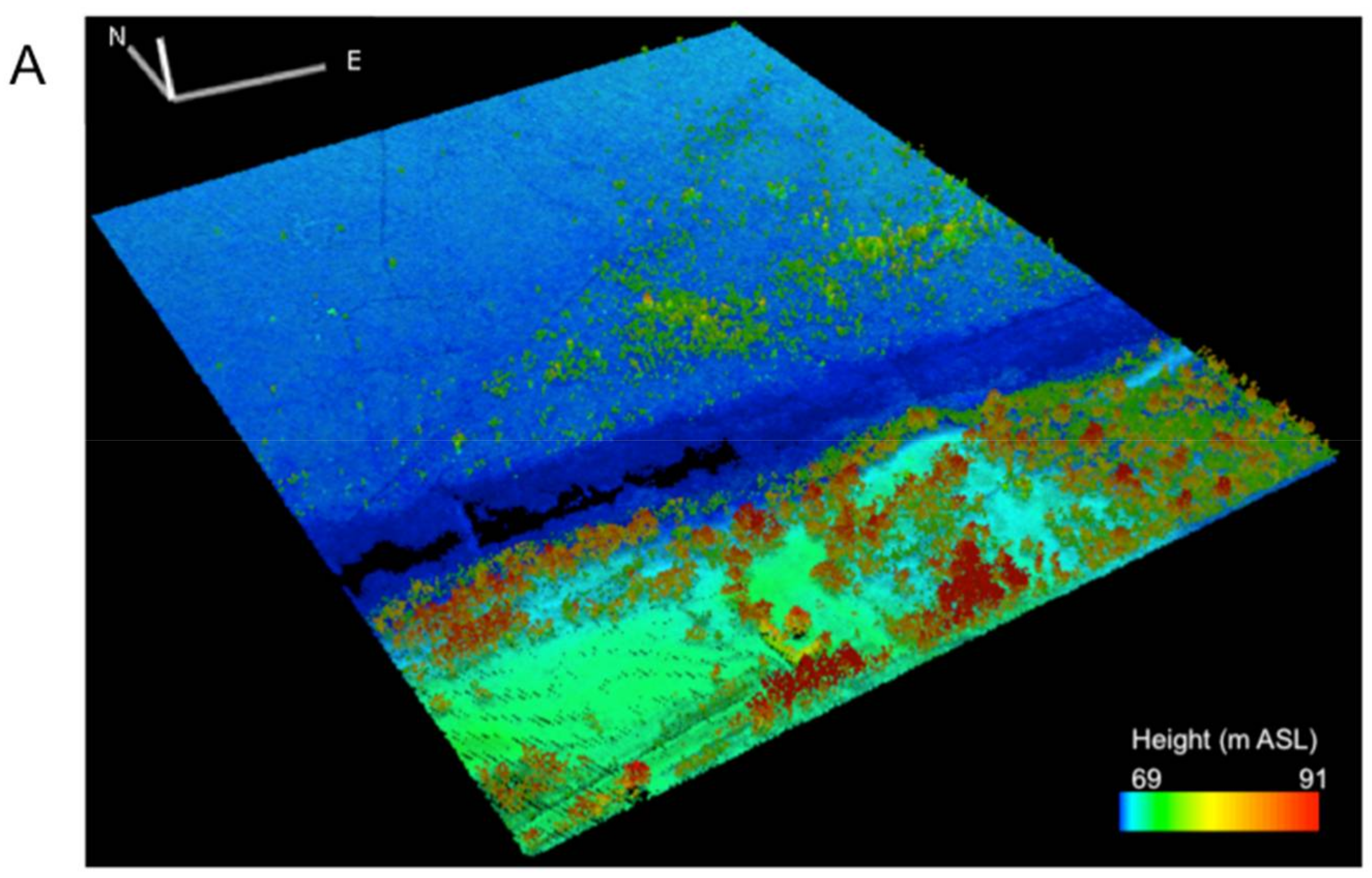
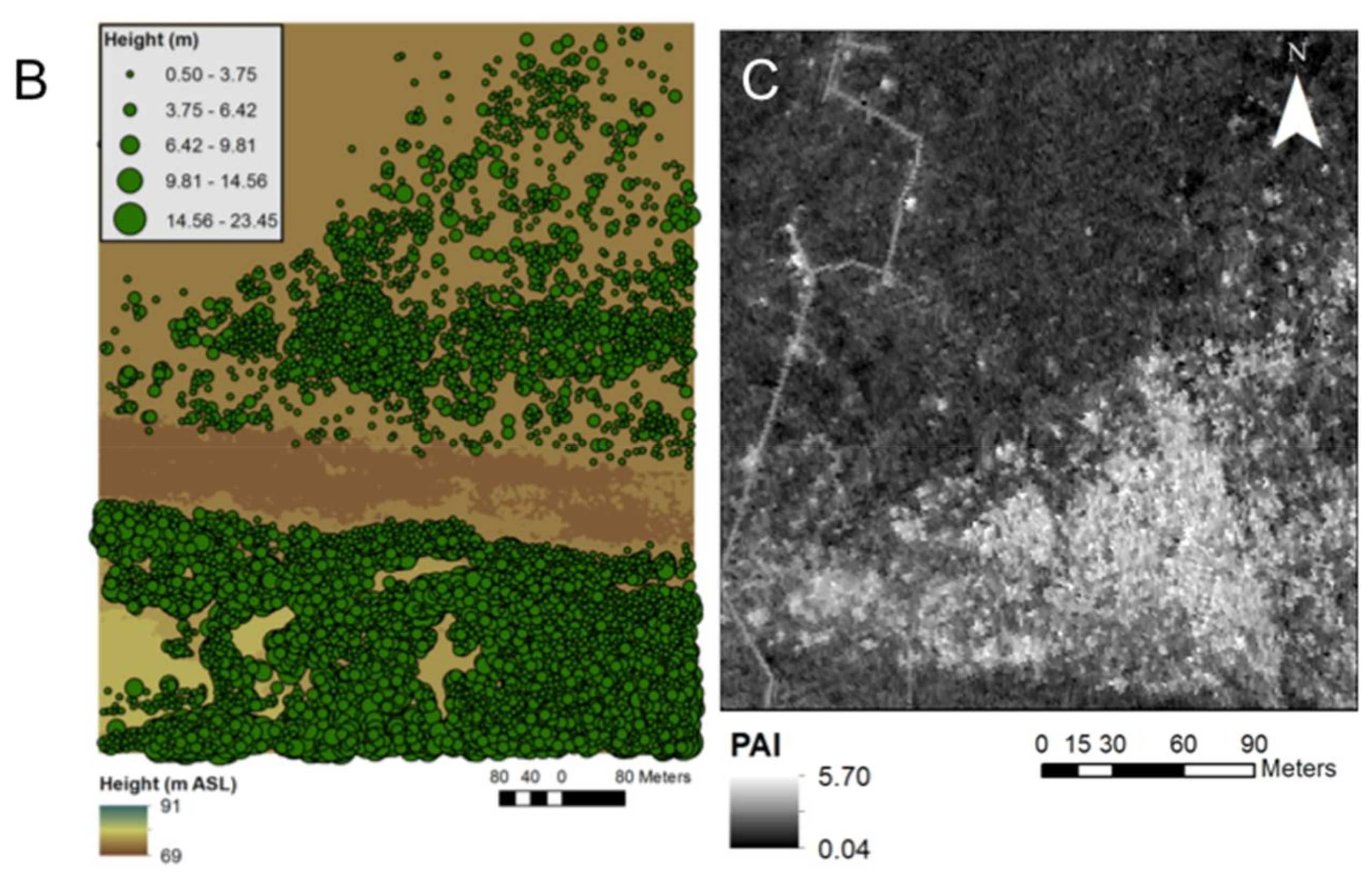
2.4.2. Tree Mask
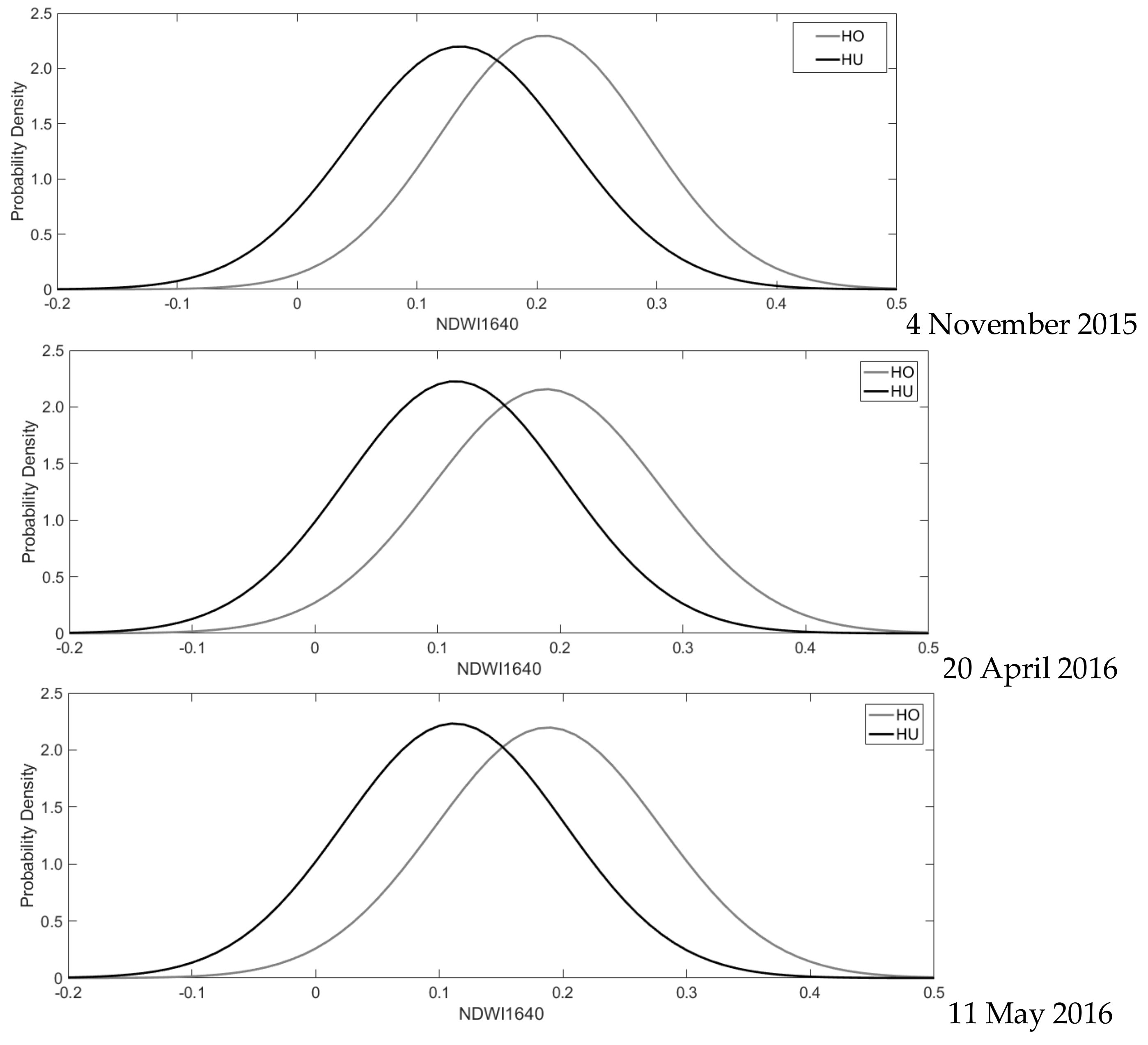
2.4.3. Hummock and Hollow Differentiation
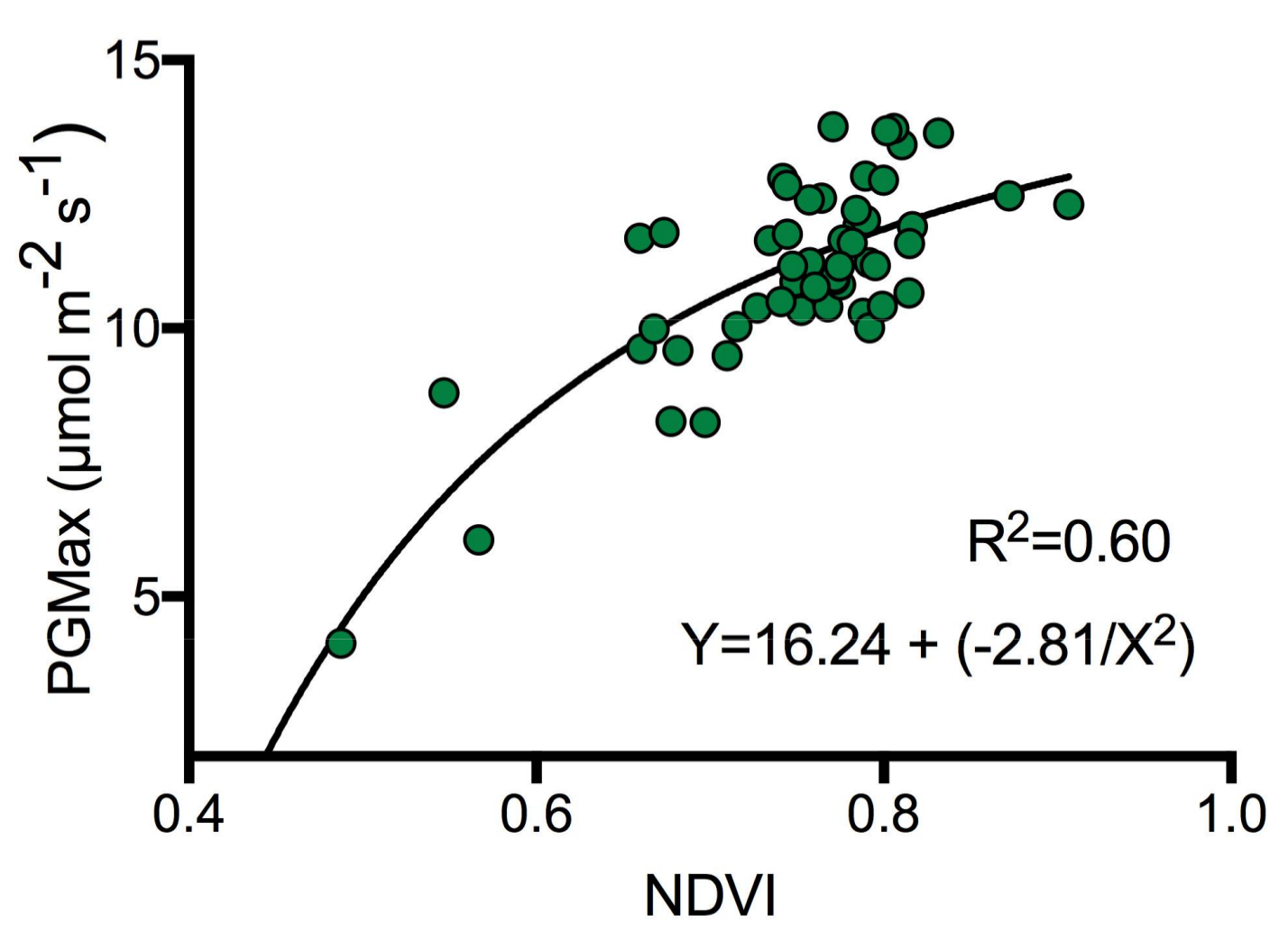
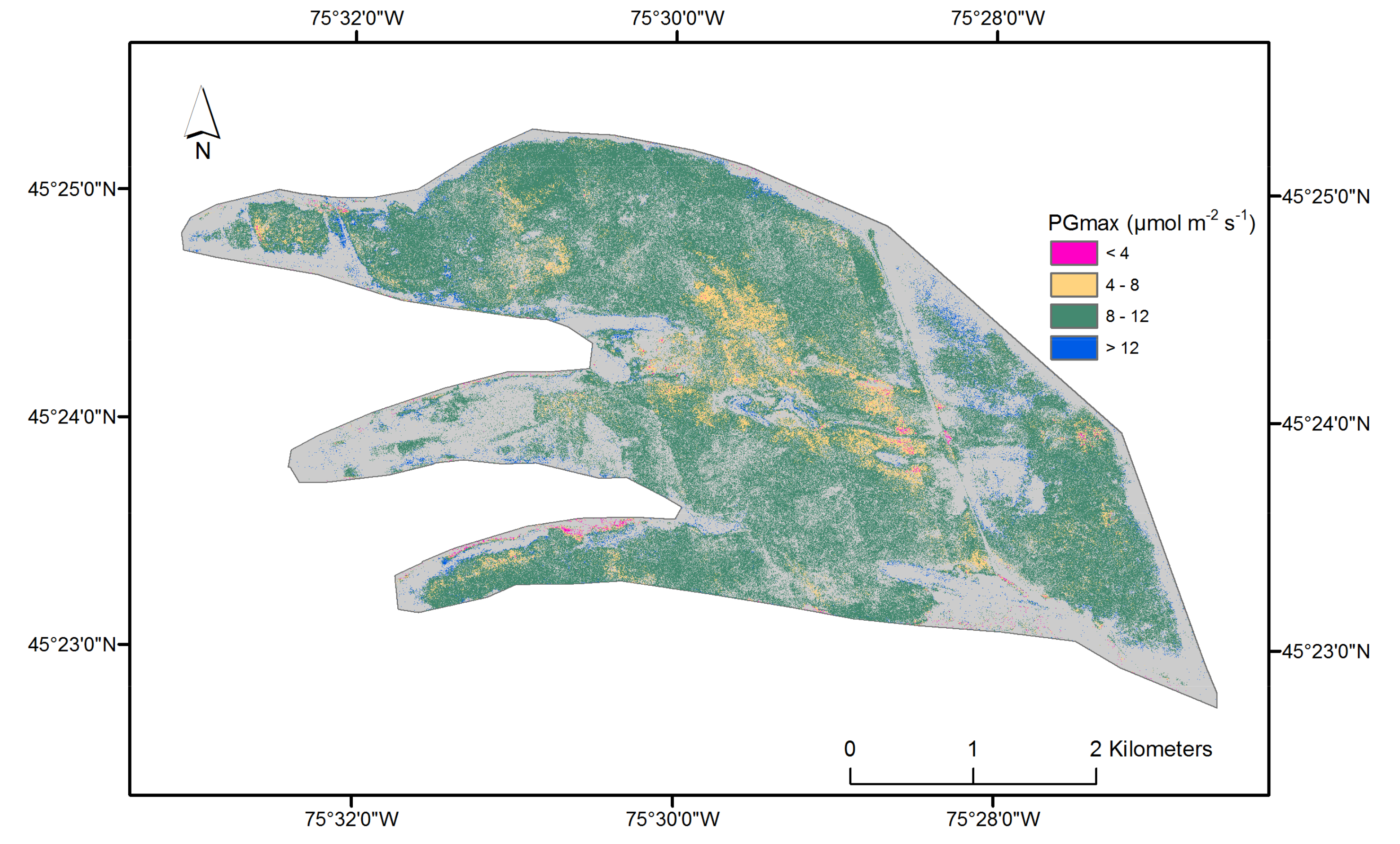
2.5. Vascular Plant (Hummocks) Light-Saturated Gross Photosynthesis (PGmax)
2.6. Near-Surface Moisture, Gravimetric Water Content, and CO2 Uptake Efficiency (Hollows)
3. Results
4. Discussion
5. Conclusions
Acknowledgments
Author Contributions
Conflicts of Interest
Appendix A


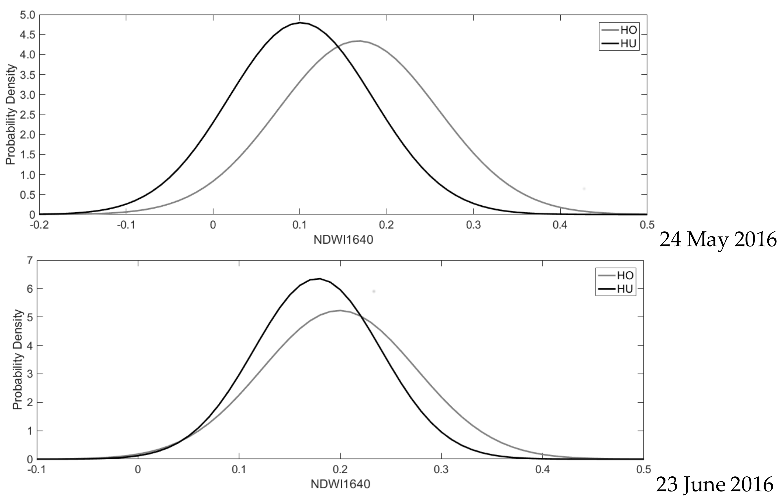
| µ (Mean) | µ-ci (95% Confidence Interval) | σ (Standard Deviation) | σ_ci (95% Confidence Interval) | |
|---|---|---|---|---|
| 4 November 2015 | ||||
| HO | 0.206 | 0.20555, 0.20577 | 0.087 | 0.08676, 0.08692 |
| HU | 0.136 | 0.13559, 0.13571 | 0.091 | 0.09066, 0.09074 |
| 20 April 2016 | ||||
| HO | 0.188 | 0.18829, 0.18852 | 0.092 | 0.09239, 0.09256 |
| HU | 0.114 | 0.11438, 0.11449 | 0.090 | 0.08951, 0.08959 |
| 11 May 2016 | ||||
| HO | 0.188 | 0.18764, 0.18786 | 0.091 | 0.09072, 0.09088 |
| HU | 0.112 | 0.11178, 0.11190 | 0.089 | 0.08933, 0.08941 |
| 24 May 2016 | ||||
| HO | 0.167 | 0.16712, 0.16735 | 0.092 | 0.09186, 0.09203 |
| HU | 0.101 | 0.10097, 0.10108 | 0.083 | 0.08315, 0.08323 |
| 23 June 2016 | ||||
| HO | 0.199 | 0.19888, 0.19908 | 0.076 | 0.07628, 0.07641 |
| HU | 0.177 | 0.17741, 0.17749 | 0.063 | 0.06280, 0.06286 |
References
- Loisel, J.; Yu, Z.; Beilman, D.W.; Camill, P.; Alm, J.; Amesbury, M.J.; Anderson, D.; Andersson, S.; Bochicchio, C.; Barber, K.; et al. A database and synthesis of northern peatland soil properties and Holocene carbon and nitrogen accumulation. Holocene 2014, 24, 1028–1042. [Google Scholar] [CrossRef] [Green Version]
- Eppinga, M.B.; Rietkerk, M.; Borren, W.; Lapshina, E.D.; Bleuten, W.; Wassen, M.J. Regular Surface Patterning of Peatlands: Confronting Theory with Field Data. Ecosystems 2008, 11, 520–536. [Google Scholar] [CrossRef]
- Belyea, L.R.; Clymo, R.S. Feedback control of the rate of peat formation. Proc. R. Soc. Lond. B Biol. Sci. 2001, 268, 1315–1321. [Google Scholar] [CrossRef] [PubMed]
- Lai, D.Y.F.; Roulet, N.T.; Humphreys, E.R.; Moore, T.R.; Dalva, M. The effect of atmospheric turbulence and chamber deployment period on autochamber CO2 and CH4 flux measurements in an ombrotrophic peatland. Biogeosciences 2012, 9, 3305–3322. [Google Scholar] [CrossRef]
- Lafleur, P.M.; Hember, R.A.; Admiral, S.W.; Roulet, N.T. Annual and seasonal variability in evapotranspiration and water table at a shrub-covered bog in southern Ontario, Canada. Hydrol. Process. 2005, 19, 3533–3550. [Google Scholar] [CrossRef]
- Moore, T.; Basiliko, N. Decomposition in Boreal Peatlands. In Boreal Peatland Ecosystems; Wieder, R.K., Vitt, D.H., Eds.; Springer: Berlin/Heidelberg, Germany, 2006; pp. 125–143. [Google Scholar]
- Murphy, M.T.; Moore, T.R. Linking root production to aboveground plant characteristics and water table in a temperate bog. Plant Soil 2010, 336, 219–231. [Google Scholar] [CrossRef]
- Talbot, J.; Roulet, N.T.; Sonnentag, O.; Moore, T.R. Increases in aboveground biomass and leaf area 85 years after drainage in a bog. Botany 2014, 92, 713–721. [Google Scholar] [CrossRef]
- Moore, T.R.; Bubier, J.L.; Bledzki, L. Litter Decomposition in Temperate Peatland Ecosystems: The Effect of Substrate and Site. Ecosystems 2007, 10, 949–963. [Google Scholar] [CrossRef]
- Rydin, H.; Jeglum, J.K. The Biology of Peatlands; Oxford University Press: Oxford, UK, 2013. [Google Scholar]
- Titus, J.E.; Wagner, D.J. Carbon Balance for Two Sphagnum Mosses: Water Balance Resolves a Physiological Paradox. Ecology 1984, 65, 1765–1774. [Google Scholar] [CrossRef]
- Titus, J.E.; Wagner, D.J.; Stephens, M.D. Contrasting Water Relations of Photosynthesis for Two Sphagnum Mosses. Ecology 1983, 64, 1109–1115. [Google Scholar] [CrossRef]
- Schipperges, B.; Rydin, H. Response of photosynthesis of Sphagnum species from contrasting microhabitats to tissue water content and repeated desiccation. New Phytol. 1998, 140, 677–684. [Google Scholar] [CrossRef]
- Harris, A.; Bryant, R.G.; Baird, A.J. Mapping the effects of water stress on Sphagnum: Preliminary observations using airborne remote sensing. Remote Sens. Environ. 2006, 100, 363–378. [Google Scholar] [CrossRef]
- Banskota, A.; Falkowski, M.J.; Smith, A.M.S.; Kane, E.S.; Meingast, K.M.; Bourgeau-Chavez, L.L.; Miller, M.E.; French, N.H. Continuous Wavelet Analysis for Spectroscopic Determination of Subsurface Moisture and Water-Table Height in Northern Peatland Ecosystems. IEEE Trans. Geosci. Remote Sens. 2017, 55, 1526–1536. [Google Scholar] [CrossRef]
- Harris, A.; Bryant, R.G. A multi-scale remote sensing approach for monitoring northern peatland hydrology: Present possibilities and future challenges. J. Environ. Manag. 2009, 90, 2178–2188. [Google Scholar] [CrossRef] [PubMed]
- Lalonde, M. The Hyperspectral Determination of Sphagnum Water Content in a Bog. Master’s Thesis, McGill University, Montreal, QC, Canada, 2013. [Google Scholar]
- Bubier, J.L.; Rock, B.N.; Crill, P.M. Spectral reflectance measurements of boreal wetland and forest mosses. J. Geophys. Res. Atmos. 1997, 102, 29483–29494. [Google Scholar] [CrossRef]
- Vogelmann, J.E.; Moss, D.M. Spectral reflectance measurements in the genus Sphagnum. Remote Sens. Environ. 1993, 45, 273–279. [Google Scholar] [CrossRef]
- Meingast, K.M.; Falkowski, M.J.; Kane, E.S.; Potvin, L.R.; Benscoter, B.W.; Smith, A.M.S.; Bourgeau-Chavez, L.L.; Miller, M.E. Spectral detection of near-surface moisture content and water-table position in northern peatland ecosystems. Remote Sens. Environ. 2014, 152, 536–546. [Google Scholar] [CrossRef]
- Arroyo-Mora, J.P.; Kalacska, M.; Lucanus, O.; Soffer, R.J.; Leblanc, G. Spectro-Spatial Relationship between UAV Derived High Resolution DEM and SWIR Hyperspectral Data: Application to an Ombrotrophic Peatland. In Proceedings of the SPIE, Warsaw, Poland, 11–14 September 2017. [Google Scholar]
- Larmola, T.; Bubier, J.L.; Kobyljanec, C.; Basiliko, N.; Juutinen, S.; Humphreys, E.; Preston, M.; Moore, T.R. Vegetation feedbacks of nutrient addition lead to a weaker carbon sink in an ombrotrophic bog. Glob. Chang. Biol. 2013, 19, 3729–3739. [Google Scholar] [CrossRef] [PubMed]
- Kalacska, M.; Arroyo-Mora, J.P.; Soffer, R.; Leblanc, G. Quality Control Assessment of the Mission Airborne Carbon 13 (MAC-13) Hyperspectral Imagery from Costa Rica. Can. J. Remote Sens. 2016, 42, 85–105. [Google Scholar] [CrossRef]
- Soffer, R.; Arroyo-Mora, J.P.; Kalacska, M.; Ifimov, G.; White, P.H.; Leblanc, S.; Nazarenko, D.; Leblanc, G. MBASSS Landsat 8 Data Product Validation Project—Final Report; National Research Council: Ottawa, ON, Canada, 2017. [Google Scholar]
- Arroyo-Mora, J.P.; Kalacska, M.; Soffer, R.J.; Ifimov, G.; Leblanc, G.; Schaaf, E.S.; Lucanus, O. Phenospectral dynamics of vegetation physiognomies at different spatial and spectral scales at the Mer Bleue ombrotrophic peatland. Remote Sens. Environ. 2018. Under Review. [Google Scholar]
- Leifeld, J.; Menichetti, L. The underappreciated potential of peatlands in global climate change mitigation strategies. Nat. Commun. 2018, 9, 1071. [Google Scholar] [CrossRef] [PubMed]
- Lafleur, P.M.; Roulet, N.T.; Admiral, S.W. Annual cycle of CO2 exchange at a bog peatland. J. Geophys. Res. Atmos. 2001, 106, 3071–3081. [Google Scholar] [CrossRef]
- Waddington, J.M.; Quinton, W.L.; Price, J.S.; Lafleur, P.M. Advances in Canadian Peatland Hydrology, 2003–2007. Can. Water Resour. J. 2009, 34, 139–148. [Google Scholar] [CrossRef]
- Moore, T.R.; Bubier, J.L.; Frolking, S.E.; Lafleur, P.M.; Roulet, N.T. Plant biomass and production and CO2 exchange in an ombrotrophic bog. J. Ecol. 2002, 90, 25–36. [Google Scholar] [CrossRef]
- Sonnentag, O.; Chen, J.M.; Roberts, D.A.; Talbot, J.; Halligan, K.Q.; Govind, A. Mapping tree and shrub leaf area indices in an ombrotrophic peatland through multiple endmember spectral unmixing. Remote Sens. Environ. 2007, 109, 342–360. [Google Scholar] [CrossRef]
- Bubier, J.L.; Moore, T.R.; Crosby, G. Fine-scale vegetation distribution in a cool temperate peatland. Can. J. Bot. 2006, 84, 910–923. [Google Scholar] [CrossRef]
- Lafleur, P.M.; Roulet, N.T.; Bubier, J.L.; Frolking, S.; Moore, T.R. Interannual variability in the peatland-atmosphere carbon dioxide exchange at an ombrotrophic bog. Glob. Biogeochem. Cycles 2003, 17, 13. [Google Scholar] [CrossRef]
- Collings, S.; Caccetta, P.; Campbell, N.; Wu, X. Techniques for BRDF Correction of Hyperspectral Mosaics. IEEE Trans. Geosci. Remote Sens. 2010, 48, 3733–3746. [Google Scholar] [CrossRef]
- Peñuelas, J.; Filella, I.; Gamon, J.A. Assessment of photosynthetic radiation-use efficiency with spectral reflectance. New Phytol. 1995, 131, 291–296. [Google Scholar] [CrossRef]
- Gamon, J.A.; Serrano, L.; Surfus, J.S. The photochemical reflectance index: An optical indicator of photosynthetic radiation use efficiency across species, functional types, and nutrient levels. Oecologia 1997, 112, 492–501. [Google Scholar] [CrossRef] [PubMed]
- Wilson, P. The Relationship Among Micro-Topographic Variation, Water Table Depth and Biogeochemistry in an Ombrotrophic Bog. Master’s Thesis, McGill University, Montreal, QC, Canada, 2012. [Google Scholar]
- Juutinen, S.; Bubier, J.L.; Moore, T.R. Responses of Vegetation and Ecosystem CO2 Exchange to 9 Years of Nutrient Addition at Mer Bleue Bog. Ecosystems 2010, 13, 874–887. [Google Scholar] [CrossRef]
- Gao, B.-. C NDWI—A normalized difference water index for remote sensing of vegetation liquid water from space. Remote Sens. Environ. 1996, 58, 257–266. [Google Scholar] [CrossRef]
- Rietkerk, M.; Dekker, S.C.; de Ruiter, P.C.; van de Koppel, J. Self-Organized Patchiness and Catastrophic Shifts in Ecosystems. Science 2004, 305, 1926–1929. [Google Scholar] [CrossRef] [PubMed]
- Lehmann, J.; Münchberger, W.; Knoth, C.; Blodau, C.; Nieberding, F.; Prinz, T.; Pancotto, V.; Kleinebecker, T. High-Resolution Classification of South Patagonian Peat Bog Microforms Reveals Potential Gaps in Up-Scaled CH4 Fluxes by use of Unmanned Aerial System (UAS) and CIR Imagery. Remote Sens. 2016, 8, 173. [Google Scholar] [CrossRef] [Green Version]
- Parent, C.; Capelli, N.; Audrey, B.; Crevècoeur, M.; Dat, J. An Overview of Plant Responses to Soil Waterlogging; Global Science Books Ltd.: Sussex, UK, 2008; Volume 2. [Google Scholar]
- Lees, K.J.; Quaife, T.; Artz, R.R.E.; Khomik, M.; Clark, J.M. Potential for using remote sensing to estimate carbon fluxes across northern peatlands—A review. Sci. Total Environ. 2018, 615, 857–874. [Google Scholar] [CrossRef] [PubMed]
- Lin, M.; Jr, H.C.L.; Shmueli, G. Research Commentary—Too Big to Fail: Large Samples and the p-Value Problem. Inf. Syst. Res. 2013, 24, 906–917. [Google Scholar] [CrossRef]
- Frolking, S.; Talbot, J.; Jones, M.C.; Treat, C.C.; Kauffman, J.B.; Tuittila, E.-S.; Roulet, N. Peatlands in the Earth’s 21st century climate system. Environ. Rev. 2011, 19, 371–396. [Google Scholar] [CrossRef]
- Wu, J.; Roulet, N.T. Climate change reduces the capacity of northern peatlands to absorb the atmospheric carbon dioxide: The different responses of bogs and fens. Glob. Biogeochem. Cycles 2014, 28, 1005–1024. [Google Scholar] [CrossRef]
- Oke, T.A.; Hager, H.A. Assessing environmental attributes and effects of climate change on Sphagnum peatland distributions in North America using single- and multi-species models. PLoS ONE 2017, 12, e0175978. [Google Scholar] [CrossRef] [PubMed]
- Waddington, J.M.; Morris, P.J.; Kettridge, N.; Granath, G.; Thompson, D.K.; Moore, P.A. Hydrological feedbacks in northern peatlands. Ecohydrology 2015, 8, 113–127. [Google Scholar] [CrossRef]
- Malhotra, A.; Roulet, N.T.; Wilson, P.; Giroux-Bougard, X.; Harris, L.I. Ecohydrological feedbacks in peatlands: An empirical test of the relationship among vegetation, microtopography and water table. Ecohydrology 2016, 9, 1346–1357. [Google Scholar] [CrossRef]
- Tarnocai, C.; Kettles, I.M.; Lacelle, B. Peatlands of Canada Database; Digital Database; Research Branch, Agriculture and Agri-Food Canada: Ottawa, ON, Canada, 2005.


| Characteristic | CASI-1500 | SASI-644 |
|---|---|---|
| Serial Number | 2511 | 3102 |
| Field of view (FOV) (°) | 39.9° | 39.7° |
| Instantaneous FOV (IFOV) (°) | 0.0270 (nadir) 0.0246 (edge) | 0.0646 (nadir) 0.0572 (edge) |
| No. cross-track pixels (detector) | 1500 | 644 |
| No. cross-track pixels (image) | 1498 | 640 |
| No. channels | 288 (max) | 160 |
| Spectral range (nm) | 375–1054 | 883–2523 |
| Spectral spacing (nm) | 2.4 | 10.0 nm @ 883 nm 12.8 nm @ 1280 nm (max) 6.2 nm @ 2523 nm |
| Spectral resolution (nm) | 3.2 | 16 nm @ 883 nm 12 nm @ 2523 nm |
| Frame rate (Frames s−1) | Programmable—Max rate dependent on # of channels | 60 Hz |
| Integration time (IT) (ms) | 1000/Frame rate | <16.67 (Typ. 2.0–6.0) |
| Focal length (FL) (pixels) | 2067.36 | 886.571 |
| Date | Heading (°) | Sun Azimuth Angle (°) Range | Sun Zenith Angle (°) Range |
|---|---|---|---|
| 4 November 2015 | 344.9 ± 1.0 | 170.2–191.6 | 61.1–62.0 |
| 20 April 2016 | 345.9 ± 1.0 | 153.6–180.3 | 33.6–36.9 |
| 11 May 2016 | 341.7 ± 0.8 | 137.6–178.0 | 27.3–33.8 |
| 24 May 2016 | 340.1 ± 1.5 | 139.2–189.6 | 24.7–29.6 |
| 23 June 2016 | 338.8 ± 0.5 | 128.6–157.9 | 23.3–30.0 |
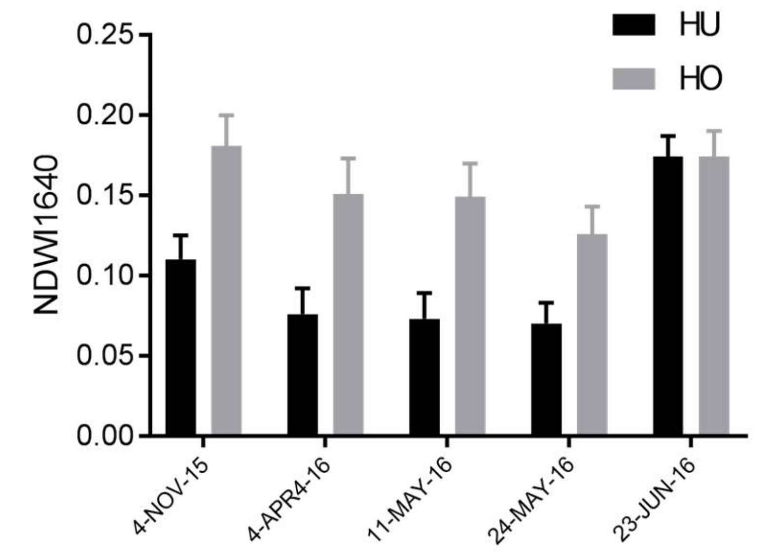
| Mean | Stdev | tstat | df | sd | ci | p-Value | |
|---|---|---|---|---|---|---|---|
| 4 November 2015 | |||||||
| HO (n = 2.40 × 10⁶) | 0.181 | 0.181 | −1104.05 | 3,838,142 | 0.0907, 0.0868 | −0.0701, −0.0699 | 0 |
| HU (n = 9.41× 10⁶) | 0.110 | 0.015 | |||||
| 20 April 2016 | |||||||
| HO (n = 2.43 × 10⁶) | 0.151 | 0.022 | −1123.08 | 3,647,862 | 0.0895, 0.0925 | −0.0741, −0.0738 | 0 |
| HU (n = 9.77 × 10⁶) | 0.076 | 0.016 | |||||
| 11 May 2016 | |||||||
| HO (n = 2.43 × 10⁶) | 0.149 | 0.021 | −1169.98 | 3,689,468 | 0.0894, 0.0908 | −0.0760, −0.0758 | 0 |
| HU (n = 9.77 × 10⁶) | 0.073 | 0.016 | |||||
| 24 May 2016 | |||||||
| HO (n = 2.43 × 10⁶) | 0.126 | 0.017 | −1023.25 | 3,484,644 | 0.0832, 0.0919 | −0.0663, −0.0661 | 0 |
| HU (n = 9.77 × 10⁶) | 0.070 | 0.013 | |||||
| 23 June 2016 | |||||||
| HO (n = 2.43 × 10⁶) | 0.174 | 0.016 | −406.85 | 3,295,761 | 0.0628, 0.0763 | −0.0216, −0.0214 | 0 |
| HU (n = 9.77 × 10⁶) | 0.174 | 0.013 | |||||
| Source | SS | df | MS | F | Prob > F |
|---|---|---|---|---|---|
| Groups | 4.6 × 10¹⁰ | 4 | 11,469,950,111 | 667,178 | 0 |
| Error | 2.1 × 10¹² | 12,120,001 | 171,917 | ||
| Total | 2.1 × 10¹² | 12,120,005 |
© 2018 by the authors. Licensee MDPI, Basel, Switzerland. This article is an open access article distributed under the terms and conditions of the Creative Commons Attribution (CC BY) license (http://creativecommons.org/licenses/by/4.0/).
Share and Cite
Arroyo-Mora, J.P.; Kalacska, M.; Soffer, R.J.; Moore, T.R.; Roulet, N.T.; Juutinen, S.; Ifimov, G.; Leblanc, G.; Inamdar, D. Airborne Hyperspectral Evaluation of Maximum Gross Photosynthesis, Gravimetric Water Content, and CO2 Uptake Efficiency of the Mer Bleue Ombrotrophic Peatland. Remote Sens. 2018, 10, 565. https://doi.org/10.3390/rs10040565
Arroyo-Mora JP, Kalacska M, Soffer RJ, Moore TR, Roulet NT, Juutinen S, Ifimov G, Leblanc G, Inamdar D. Airborne Hyperspectral Evaluation of Maximum Gross Photosynthesis, Gravimetric Water Content, and CO2 Uptake Efficiency of the Mer Bleue Ombrotrophic Peatland. Remote Sensing. 2018; 10(4):565. https://doi.org/10.3390/rs10040565
Chicago/Turabian StyleArroyo-Mora, J. Pablo, Margaret Kalacska, Raymond J. Soffer, Tim R. Moore, Nigel T. Roulet, Sari Juutinen, Gabriela Ifimov, George Leblanc, and Deep Inamdar. 2018. "Airborne Hyperspectral Evaluation of Maximum Gross Photosynthesis, Gravimetric Water Content, and CO2 Uptake Efficiency of the Mer Bleue Ombrotrophic Peatland" Remote Sensing 10, no. 4: 565. https://doi.org/10.3390/rs10040565