Simplified Normalization of C-Band Synthetic Aperture Radar Data for Terrestrial Applications in High Latitude Environments


Abstract
:1. Introduction
2. Material
2.1. Sentinel-1
2.2. Envisat ASAR GM Frozen Surface Backscatter Dataset
2.3. Digital Elevation Models
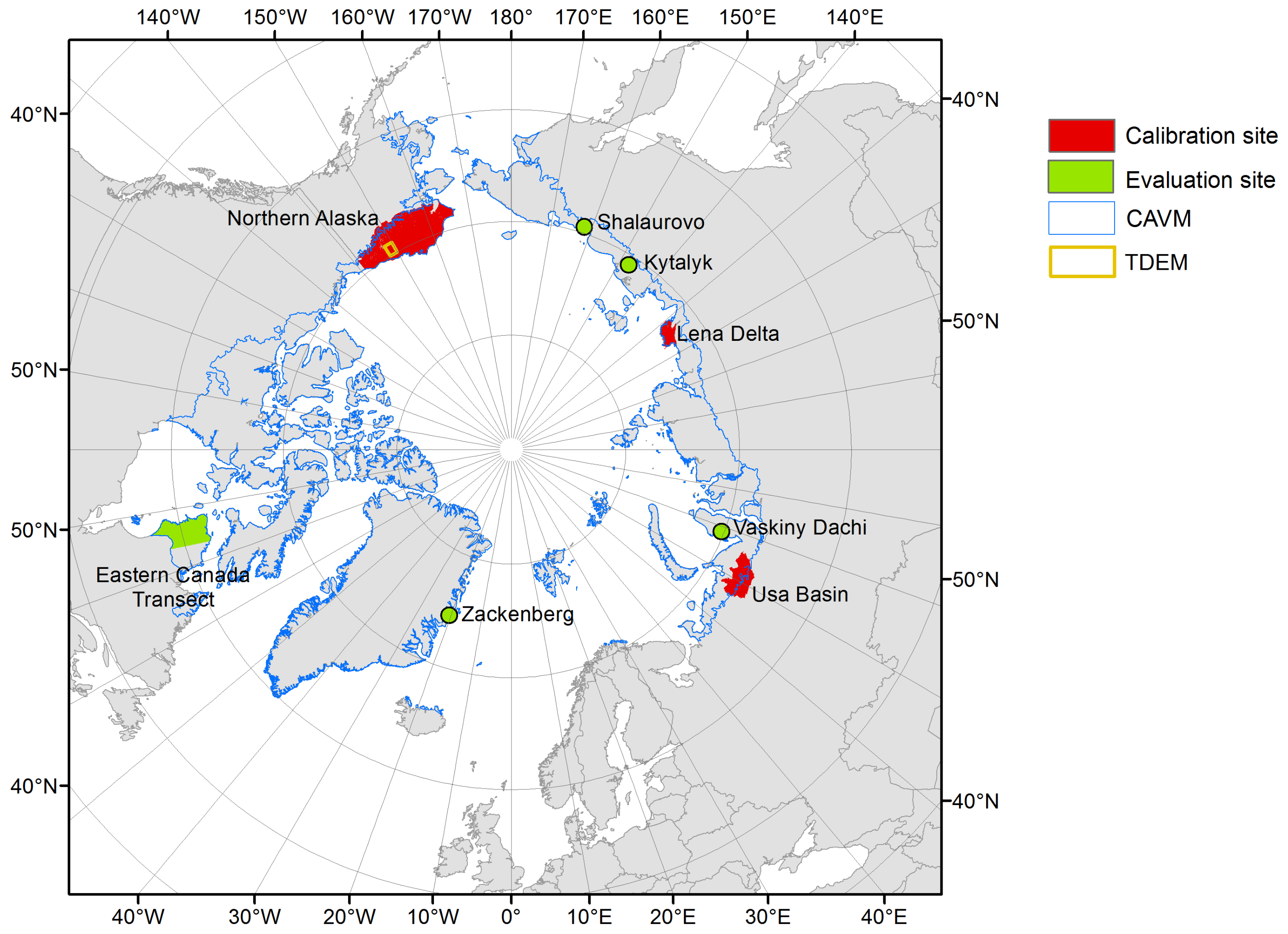
2.4. Land Cover Data and Focus Regions
2.4.1. Lena Delta
2.4.2. Usa Basin
2.4.3. Ecosystems Map of Northern Alaska
2.4.4. Circumpolar Arctic Vegetation Map
2.4.5. Evaluation Sites
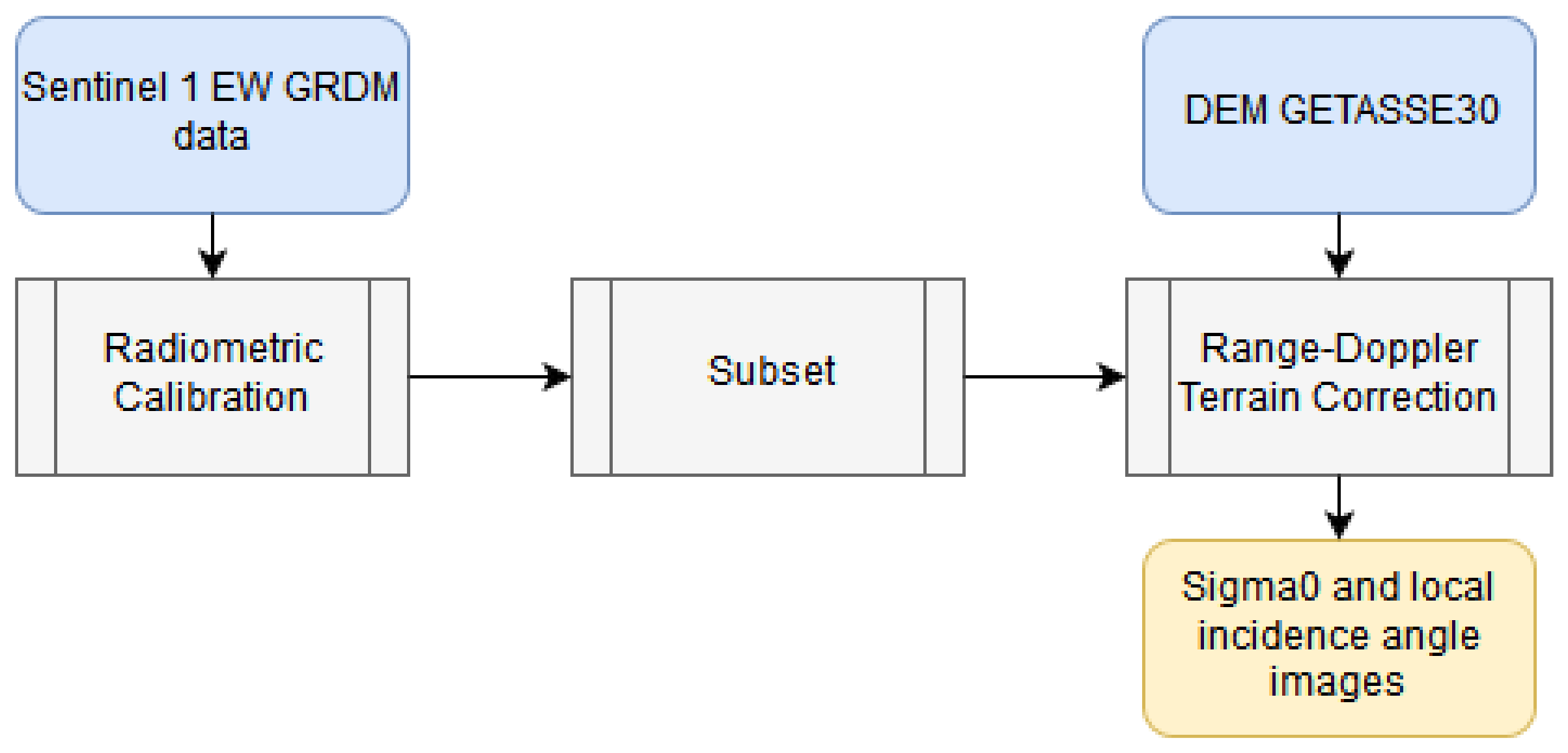
3. Methodology
4. Results
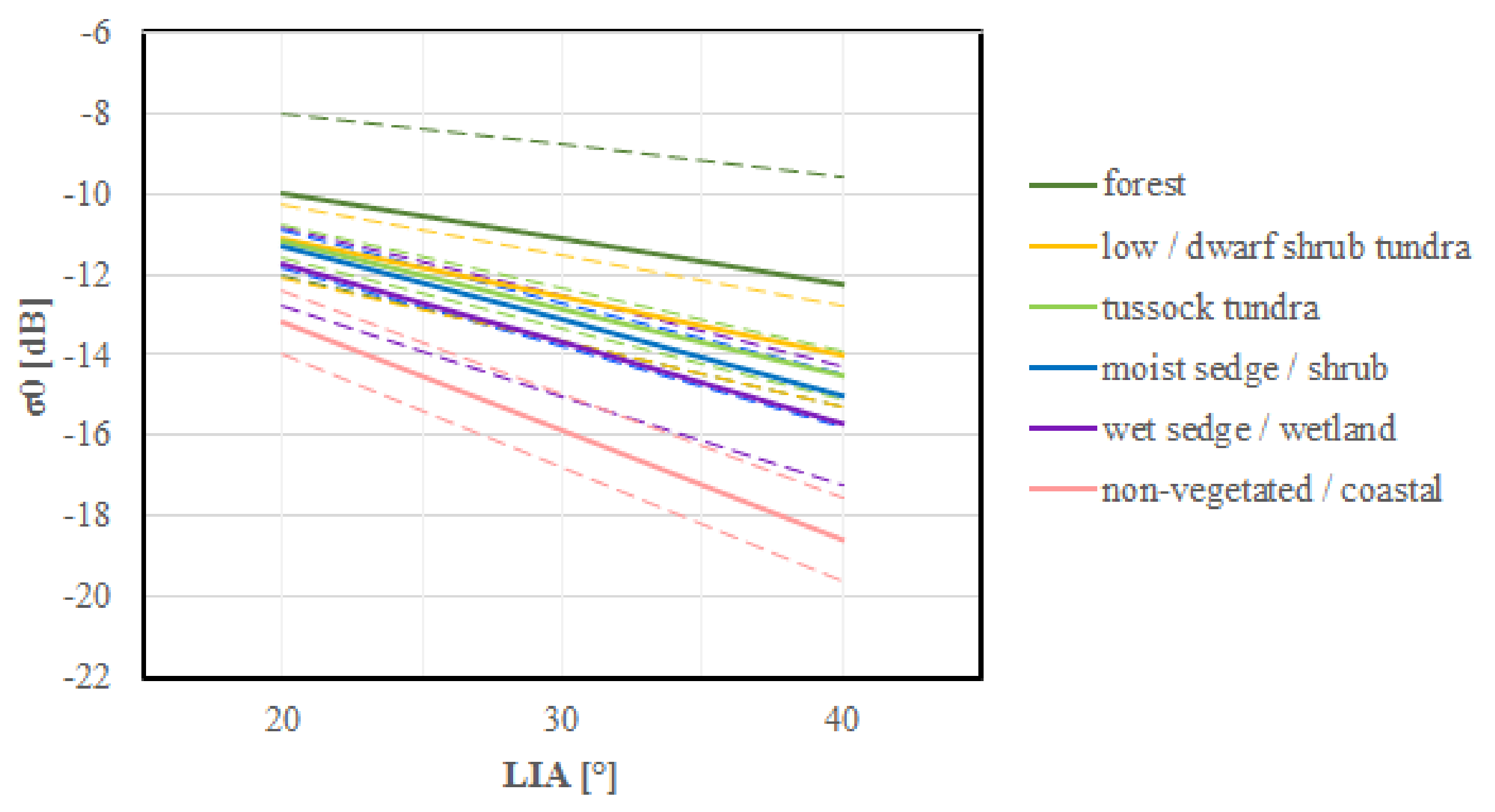
4.1. Normalization
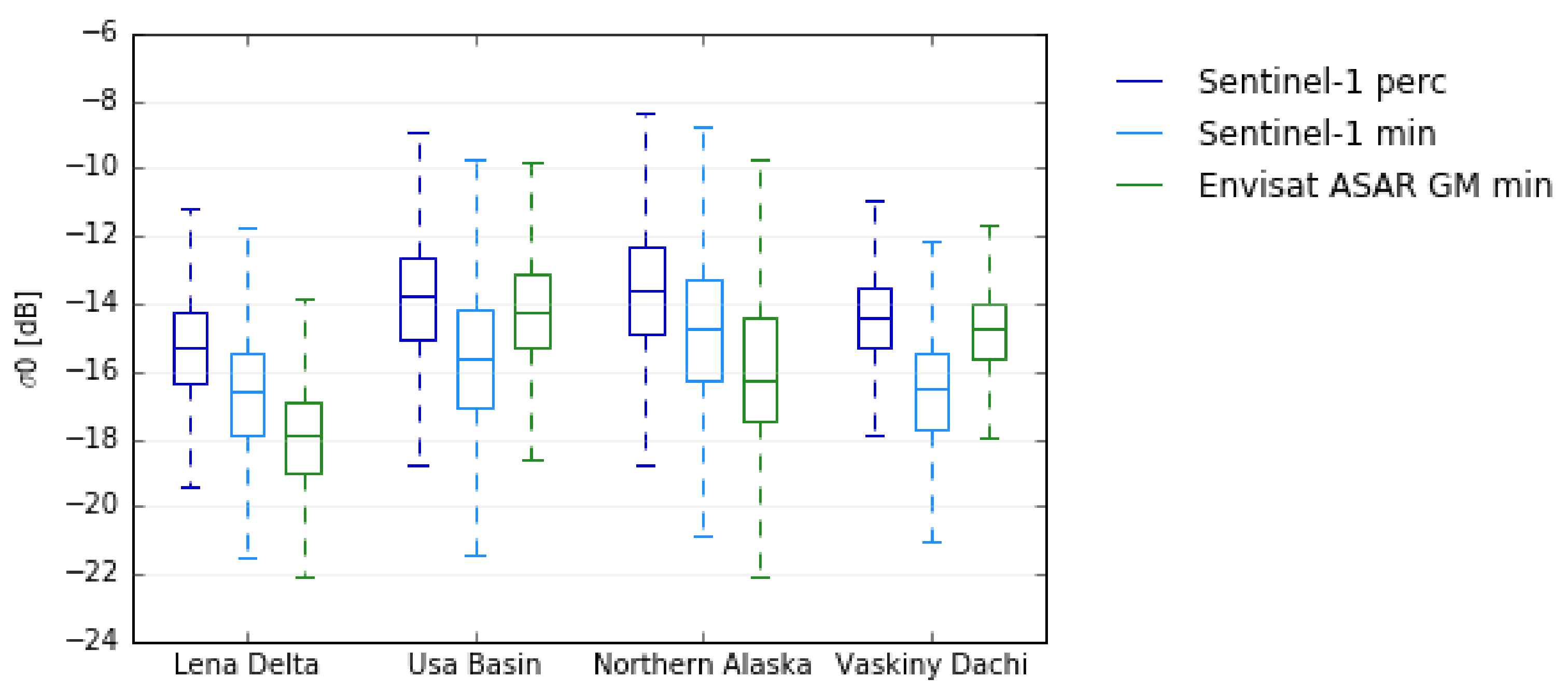
4.2. Sentinel-1 Frozen Surface Backscatter Statistics
5. Discussion
5.1. Normalization
5.2. Sentinel-1 Frozen Surface Backscatter Statistics
6. Conclusions
Acknowledgments
Author Contributions
Conflicts of Interest
References
- Ulaby, F.T.; Moore, R.K.; Fung, A. Microwave Remote Sensing—Active and Passive; Artech House: Norwood, MA, USA, 1982; Volume II. [Google Scholar]
- Mladenova, I.E.; Jackson, T.J.; Bindlish, R.; Hensley, S. Incidence Angle Normalization of Radar Backscatter Data. IEEE Trans. Geosci. Remote Sens. 2013, 51, 1791–1804. [Google Scholar] [CrossRef]
- Wickel, A.J.; Jackson, T.J.; Wood, E.F. Multitemporal monitoring of soil moisture with RADARSAT SAR during the 1997 Southern Great Plains hydrology experiment. Int. J. Remote Sens. 2001, 22, 1571–1583. [Google Scholar] [CrossRef]
- Loew, A.; Ludwig, R.; Mauser, W. Derivation of Surface Soil Moisture From ENVISAT ASAR Wide Swath and Image Mode Data in Agricultural Areas. IEEE Trans. Geosci. Remote Sens. 2006, 44, 889–899. [Google Scholar] [CrossRef]
- Pathe, C.; Wagner, W.; Sabel, D.; Doubkova, M.; Basara, J.B. Using ENVISAT ASAR Global Mode Data for Surface Soil Moisture Retrieval Over Oklahoma, USA. IEEE Trans. Geosci. Remote Sens. 2009, 47, 468–480. [Google Scholar] [CrossRef]
- Baup, F.; Mougin, E.; Hiernaux, P.; Lopes, A.; Rosnay, P.D.; Chenerie, I. Radar Signatures of Sahelian Surfaces in Mali Using ENVISAT-ASAR Data. IEEE Trans. Geosci. Remote Sens. 2007, 45, 2354–2363. [Google Scholar] [CrossRef] [Green Version]
- Van Doninck, J.; Wagner, W.; Melzer, T.; Baets, B.D.; Verhoest, N.E.C. Seasonality in the Angular Dependence of ASAR Wide Swath Backscatter. IEEE Geosci. Remote Sens. Soc. 2014, 11, 1423–1427. [Google Scholar] [CrossRef]
- Bartsch, A.; Pointner, G.; Leibman, M.O.; Dvornikov, Y.A.; Khomutov, A.V.; Trofaier, A.M. Circumpolar Mapping of Ground-Fast Lake Ice. Front. Earth Sci. 2017, 5. [Google Scholar] [CrossRef]
- Mäkynen, M.P.; Manninen, A.T.; Similä, M.H.; Karvonen, J.A.; Hallikainen, M.T. Incidence Angle Dependence of the Statistical Properties of C-Band HH-Polarization Backscattering Signatures of the Baltic Sea Ice. IEEE Geosci. Remote Sens. Soc. 2002, 40, 2593–2605. [Google Scholar] [CrossRef]
- Frison, P.L.; Mougin, E. Use of ERS-1 wind scatterometer data over land surfaces. IEEE Geosci. Remote Sens. Soc. 1996, 34, 550–560. [Google Scholar] [CrossRef]
- Menges, C.H.; Van Zyl, J.J.; Hill, G.J.E.; Ahmad, W. A procedure for the correction of the eVect of variation in incidence angle on AIRSAR data. Int. J. Remote Sens. 2001, 22, 829–841. [Google Scholar] [CrossRef]
- Bartsch, A.; Trofaier, A.; Hayman, G.; Sabel, D.; Schlaffer, S.; Clark, D.; Blyth, E. Detection of Open Water Dynamics with ENVISAT ASAR in Support of Land Surface Modelling at High Latitudes. Biogeosciences 2012, 9, 703–714. [Google Scholar] [CrossRef] [Green Version]
- Widhalm, B.; Bartsch, A.; Heim, B. A novel approach for the characterization of tundra wetland regions with C-band SAR satellite data. Int. J. Remote Sens. 2015, 36, 5537–5556. [Google Scholar] [CrossRef] [PubMed] [Green Version]
- Bartsch, A.; Widhalm, B.; Kuhry, P.; Hugelius, G.; Palmtag, J.; Siewert, M.B. Can C-band synthetic aperture radar be used to estimate soil organic carbon storage in tundra? Biogeosciences 2016, 13, 5453–5470. [Google Scholar] [CrossRef]
- Bartsch, A.; Höfler, A.; Kroisleitner, C.; Trofaier, A.M. Land Cover Mapping in Northern High Latitude Permafrost Regions with Satellite Data: Achievements and Remaining Challenges. Remote Sens. 2016, 8, 979. [Google Scholar] [CrossRef]
- Attema, E.; Bargellini, P.; Edwards, P.; Levrini, G.; Lokas, S.; Moeller, L.; Rosich-Tell, B.; Secchi, P.; Torres, R.; Davidson, M.; et al. Sentinel-1: The Radar Mission for GMES Operational Land and Sea Services. ESA Bull. 2007, 131, 10–17. [Google Scholar]
- Potin, P. Sentinel-1 User Handbook; European Space Agency (ESA): Paris, France, 2013. [Google Scholar]
- Torres, R.; Snoeij, P.; Geudtner, D.; Bibby, D.; Davidson, M.; Attema, E.; Potin, P.; Rommen, B.; Floury, N.; Brown, M.; et al. GMES Sentinel-1 mission. Remote Sens. Environ. 2012, 120, 9–24. [Google Scholar] [CrossRef]
- Lehner, B.; Döll, P. Development and Validation of a Global Database of Lakes, Reservoirs and Wetlands. J. Hydrol. 2004, 296, 1–22. [Google Scholar] [CrossRef]
- Bicheron, P.; Defourny, P.; Brockmann, C.; Schouten, L.; Vancutsem, C.; Huc, M.; Bontemps, S. GlobCover: Products Description and Validation Report; Technical Report; MEDIASFrance: Toulouse, France, 2008. [Google Scholar]
- Walker, D.; Gould, W.; Maier, H.; Raynolds, M. The Circumpolar Arctic Vegetation Map: AVHRR-derived base maps, environmental controls, and integrated mapping procedures. Int. J. Remote Sens. 2002, 23, 4551–4570. [Google Scholar] [CrossRef]
- Santoro, M.; Strozzi, T. Circumpolar digital elevation models >55∘N with links to geotiff images. PANGAEA 2012. [Google Scholar] [CrossRef]
- Schneider, J.; Grosse, G.; Wagner, D. Land cover classification of tundra environments in the Arctic Lena Delta based on Landsat 7 ETM+ data and its application for upscaling of methane emissions. Remote Sens. Environ. 2009, 113, 380–391. [Google Scholar] [CrossRef] [Green Version]
- Virtanen, T.; Mikkola, K.; Nikula, A. Satellite image based vegetation classification of a large area using limited ground reference data: A case study in the Usa Basin, north-east European Russia. Polar Res. 2004, 23, 51–66. [Google Scholar] [CrossRef]
- Jorgenson, M.T.; Heiner, M. Ecosystems of Northern Alaska; Unpublished 1:2.5 Million-Scale Map; ABR, Inc.: Fairbanks, AK, USA, 2003. [Google Scholar]
- Bartsch, A.; Grosse, G.; Kääb, A.; Westermann, S.; Strozzi, T.; Wiesmann, A.; Duguay, C.; Seifert, F.M.; Obu, J.; Goler, R. GlobPermafrost How space-based earth observation supports understanding of permafrost. In Proceedings of the ESA Living Planet Symposium 2016, Prague, Czech Republic, 9–13 May 2016; p. 6. [Google Scholar]
- Palmtag, J.; Hugelius, G.; Lashchinskiy, N.; Tamstorf, M.P.; Richter, A.; Elberling, B.; Kuhry, P. Storage, Landscape Distribution, and Burial History of Soil Organic Matter in Contrasting Areas of Continuous Permafrost. Arct. Antarct. Alp. Res. 2015, 47, 71–88. [Google Scholar] [CrossRef]
- Siewert, M.B.; Hanisch, J.; Weiss, N.; Kuhry, P.; Maximov, T.C.; Hugelius, G. Comparing carbon storage of Siberian tundra and taiga permafrost ecosystems at very high spatial resolution. J. Geophys. Res. Biogeosci. 2015, 120, 1973–1994. [Google Scholar] [CrossRef]
- Leibman, M.; Khomutov, A.; Gubarkov, A.; Mullanurov, D.; Dvornikov, Y. The research station Vaskiny Dachi, Central Yamal, West Siberia, Russia A review of 25 years of permafrost studies. Fennia 2015, 193, 3–30. [Google Scholar]
- Khomutov, A.; Leibman, M. Landslides in Cold Regions in the Context of Climate Change; Chapter Assessment of Landslide Hazards in a Typical Tundra of Central Yamal, Russia; Springer International Publishing: Cham, Switzerland, 2014; pp. 271–290. [Google Scholar]
- Quebec Ministry of Natural Resources. Vegetation Zones and Bioclimatic Domains of the Quebec Province; Quebec Ministry of Natural Resources: Quebec, QC, Canada, 2003.
- Lemieux, J.M.; Fortier, R.; Talbot-Poulin, M.C.; Molson, J.; Therrien, R.; Ouellet, M.; Banville, D.; Coch, M.; Murray, R. Groundwater occurrence in cold environments: Examples from Nunavik, Canada. Hydrol. J. 2016, 24, 1497–1513. [Google Scholar] [CrossRef]
- Hachem, S.; Allard, M.; Duguay, C. Using the MODIS land surface temperature product for mapping permafrost: An application to northern Québec and Labrador, Canada. Permafr. Periglac. Process. 2009, 20. [Google Scholar] [CrossRef]
- Mougin, E.; Lopes, A.; Frison, P.L.; Proisy, C. Preliminary analysis of ERS-1 wind scatterometer data over land surfaces. Int. J. Remote Sens. 1995, 16, 391–398. [Google Scholar] [CrossRef]
- Woodhouse, I. Introduction to Microwave Remote Sensing; Taylor & Francis: New York, NY, USA, 2006. [Google Scholar]
- Bergstedt, H.; Zwieback, S.; Bartsch, A.; Leibman, M. Dependence of C-Band Backscatter on Ground Temperature, Air Temperature and Snow Depth in Arctic Permafrost Regions. Remote Sens. 2018, 10, 142. [Google Scholar] [CrossRef]
- Naeimi, V.; Paulik, C.; Bartsch, A.; Wagner, W.; Kidd, R.; Boike, J.; Elger, K. ASCAT Surface State Flag (SSF): Extracting Information on Surface Freeze/Thaw Conditions from Backscatter Data Using an Empirical Threshold-Analysis Algorithm. IEEE Trans. Geosci. Remote Sens. 2012, 50, 2566–2582. [Google Scholar] [CrossRef]
- Bergstedt, H.; Bartsch, A. Surface State across Scales; Temporal and Spatial Patterns in Land Surface Freeze/Thaw Dynamics. Geosciences 2017, 7, 65. [Google Scholar] [CrossRef]
- CAVM Team. Circumpolar Arctic Vegetation Map; (1:7,500,000 Scale), Conservation of Arctic Flora and Fauna (CAFF) Map No. 1; U.S. Fish and Wildlife Service: Anchorage, AK, USA, 2003.
- Gauthier, Y.; Bernier, M.; Fortin, J.P. Aspect and incidence angle sensitivity in ERS-1 SAR data. Int. J. Remote Sens. 1998, 19, 2001–2006. [Google Scholar] [CrossRef]
- Forbes, B.C.; Kumpula, T.; Meschtyb, N.; Laptander, R.; Macias-Fauria, M.; Zetterberg, P.; Verdonen, M.; Skarin, A.; Kim, K.Y.; Boisvert, L.N.; et al. Sea ice, rain-on-snow and tundra reindeer nomadism in Arctic Russia. Biol. Lett. 2016, 12. [Google Scholar] [CrossRef] [PubMed]
- Kumpula, T.; Forbes, B.C.; Stammler, F.; Meschtyb, N. Dynamics of a Coupled System: Multi-Resolution Remote Sensing in Assessing Social-Ecological Responses during 25 Years of Gas Field Development in Arctic Russia. Remote Sens. 2012, 4, 1046–1068. [Google Scholar] [CrossRef]
- Bartsch, A. Ten Years of SeaWinds on QuikSCAT for Snow Applications. Remote Sens. 2010, 2, 1142–1156. [Google Scholar] [CrossRef]
- Muster, S.; Langer, M.; Heim, B.; Westermann, S.; Boike, J. Subpixel heterogeneity of ice-wedge polygonal tundra: A multi-scale analysis of land cover and evapotranspiration in the Lena River Delta, Siberia. Tellus B Chem. Phys. Meteorol. 2012, 64. [Google Scholar] [CrossRef]


| () | s () | # Asc | # Desc | # Scenes | ||
|---|---|---|---|---|---|---|
| Usa Basin ★ | 0.9 | 22.8 | 7.7 | 10 | 9 | 84 |
| Lena Delta ★ | 0.2 | 14.2 | 5.0 | 0 | 8 | 44 |
| Northern Alaska ★ ⋄ | 4.0 | 34.3 | 4.9 | 13 | 9 | 82 |
| Zackenberg • | 6.0 | 31.8 | 11.7 | 11 | 2 | 66 |
| Kytalyk | 0.0 | 0.1 | 3.0 | 0 | 4 | 11 |
| East Canada Transect | 0.7 | 19.0 | 3.5 | 6 | 3 | 32 |
| Vaskiny Dachi | 0.3 | 1.8 | 10.8 | 7 | 7 | 90 |
| Shalaurovo | 0.9 | 2.8 | 3.0 | 0 | 3 | 15 |
| Landcover Class | k | d | R | Height | Merged Class |
|---|---|---|---|---|---|
| Usa Basin | |||||
| Spruce forest | −0.08 | −8.81 | 0.11 | high | Forest |
| Pine forest | −0.16 | −7.82 | 0.22 | high | Forest |
| Mixed forest | −0.09 | −8.67 | 0.12 | high | Forest |
| young stands | −0.09 | −8.54 | 0.11 | high | |
| Willow-complexes | −0.12 | −8.16 | 0.17 | high | |
| Meadows | −0.12 | −7.58 | 0.19 | medium | |
| Bog shrubland | −0.12 | −8.39 | 0.17 | medium | |
| Open bogs | −0.14 | −8.45 | 0.21 | low | wet sedge/wetland |
| Wetlands | −0.16 | −8.05 | 0.24 | low | wet sedge/wetland |
| Shrub-moss tundra | −0.14 | −8.96 | 0.22 | medium | low/ dwarf shrub tundra |
| Dwarf birch tundra | −0.13 | −9.19 | 0.21 | medium | low/ dwarf shrub tundra |
| Shrub-lichen tundra | −0.16 | −8.78 | 0.25 | medium | low/ dwarf shrub tundra |
| dry tundra with some bare peat | −0.16 | −8.77 | 0.27 | low | |
| sparse alpine tundra | −0.12 | −8.83 | 0.12 | other | |
| bare land | −0.07 | −8.79 | 0.03 | other | |
| anthropogenic | −0.13 | −7.25 | 0.09 | other | |
| human impacted tundra-shrublands | −0.10 | −9.47 | 0.15 | other | |
| Northern Alaska | |||||
| Coastal Barrens | −0.24 | −8.78 | 0.27 | low | non-vegetated/coastal |
| Coastal Wet Sedge Tundra | −0.23 | −8.37 | 0.31 | low | wet sedge/wetland |
| Coastal Grass & Dwarf Shrub Tundra | −0.22 | −7.76 | 0.31 | medium | low/ dwarf shrub tundra |
| Riverine Dryas Dwarf Shrub Tundra | −0.08 | −8.72 | 0.08 | medium | low/ dwarf shrub tundra |
| Riverine Barrens | −0.18 | −6.67 | 0.17 | other | |
| Riverine Low Willow Shrub | −0.17 | −6.20 | 0.29 | medium | low/ dwarf shrub tundra |
| Riverine Moist Sedge Shrub | −0.18 | −7.48 | 0.24 | medium | moist sedge/shrub |
| Riverine Wet Sedge Tundra | −0.21 | −7.17 | 0.25 | low | wet sedge/wetland |
| Riverine Spruce-Balsam Poplar Forest | −0.17 | −6.01 | 0.31 | high | Forest |
| Riverine Balsam Poplar Forest | −0.16 | −5.83 | 0.38 | high | Forest |
| Riverine Spruce Forest | −0.07 | −8.85 | 0.07 | high | Forest |
| Riverine Tall Alder-Willow Scrub | −0.10 | −7.66 | 0.14 | medium | |
| Lowland Wet Sedge Tundra | −0.24 | −6.70 | 0.40 | low | wet sedge/wetland |
| Lowland Moist Sedge Tundra | −0.23 | −6.52 | 0.46 | low | moist sedge/shrub |
| Lowland Low Birch-Willow Shrub | −0.15 | −8.34 | 0.23 | medium | low/ dwarf shrub tundra |
| Lowland Spruce Forest | −0.17 | −5.91 | 0.43 | high | Forest |
| Upland Birch-Aspen Forest | −0.08 | −8.14 | 0.08 | high | Forest |
| Upland Tussock Tundra | −0.18 | −7.38 | 0.37 | medium | tussock tundra |
| Upland Dryas Dwarf Shrub Tundra | −0.13 | −7.65 | 0.10 | medium | low/ dwarf shrub tundra |
| Upland Shrubby Tussock Tundra | −0.15 | −8.32 | 0.26 | medium | tussock tundra |
| Upland Low Birch-Willow Shrub | −0.12 | −8.85 | 0.15 | medium | low/ dwarf shrub tundra |
| Upland Moist Sedge Shrub | −0.13 | −8.80 | 0.15 | medium | moist sedge/shrub |
| Upland Birch-Aspen-Spruce Forest | −0.07 | −8.82 | 0.07 | high | Forest |
| Upland Spruce Forest | −0.09 | −8.18 | 0.11 | high | Forest |
| Upland Tall Alder Shrub | −0.07 | −8.18 | 0.07 | medium | |
| Alpine Carbonate Barrens | −0.06 | −5.73 | 0.04 | other | |
| Alpine Mafic Barrens | −0.14 | −5.13 | 0.18 | other | |
| Alpine Non-Carbonate Dryas Dwarf Shrub | −0.09 | −8.39 | 0.07 | medium | |
| Alpine Carbonate Dryas Dwarf Shrub | −0.07 | −6.44 | 0.04 | medium | |
| Alpine Mafic Dryas Dwarf Shrub | −0.14 | −5.40 | 0.19 | medium | |
| Lena Delta | |||||
| Mainly non-vegetated areas | −0.30 | −6.84 | 0.44 | low | non-vegetated/coastal |
| Dry moss-, sedge-, and dwarf shrub-dominated tundra | −0.23 | −7.74 | 0.51 | low | |
| Wet, sedge- and moss-dominated tundra | −0.20 | −7.93 | 0.37 | low | wet sedge/wetland |
| Dry, grass-dominated tundra | −0.21 | −7.61 | 0.37 | low | |
| Moist grass- and moss-dominated tundra | −0.19 | −7.85 | 0.46 | low | moist sedge/shrub |
| Moist to dry dwarf shrub-dominated tundra | −0.20 | −7.34 | 0.39 | medium | moist sedge/shrub |
| Dry tussock tundra | −0.19 | −7.68 | 0.46 | medium |
| Usa Basin | Lena Delta | Northern Alaska | Zacken-Berg | Kytalyk | East Canada Transect | Vaskiny Dachi | Shalau-Rovo | |
|---|---|---|---|---|---|---|---|---|
| Sedge/grass, moss wetland | 5493 | 7395 | ||||||
| Sedge, moss, dwarf-shrub wetland | 17,904 | 40,384 | ||||||
| Sedge, moss, low-shrub wetland | 4517 | 1579 | 1633 | |||||
| Graminoid, prostrate dwarf-shrub, forb tundra | 12,147 | |||||||
| Nontussock sedge, dwarf-shrub, moss tundra | 687 | 117 | 32,445 | 21,720 | 165 | |||
| Tussock-sedge, dwarf-shrub, moss tundra | 102,517 | 27 | 90 | |||||
| Erect dwarf-shrub tundra | 9381 | 2744 | 34,711 | 27 | 79,630 | 189 | ||
| Low-shrub tundra | 37,354 | 2038 | 16,099 | 904 | ||||
| Prostrate dwarf-shrub, herb tundra | 2418 | |||||||
| Prostrate/Hemiprostrate dwarf-shrub tundra | 35 | |||||||
| Cryptogam barren complex (bedrock) | 10,551 | |||||||
| Noncarbonate mountain complex | 701 | 29,372 | 92 | |||||
| Carbonate mountain complex | 2193 | 43,613 |
© 2018 by the authors. Licensee MDPI, Basel, Switzerland. This article is an open access article distributed under the terms and conditions of the Creative Commons Attribution (CC BY) license (http://creativecommons.org/licenses/by/4.0/).
Share and Cite
Widhalm, B.; Bartsch, A.; Goler, R. Simplified Normalization of C-Band Synthetic Aperture Radar Data for Terrestrial Applications in High Latitude Environments. Remote Sens. 2018, 10, 551. https://doi.org/10.3390/rs10040551
Widhalm B, Bartsch A, Goler R. Simplified Normalization of C-Band Synthetic Aperture Radar Data for Terrestrial Applications in High Latitude Environments. Remote Sensing. 2018; 10(4):551. https://doi.org/10.3390/rs10040551
Chicago/Turabian StyleWidhalm, Barbara, Annett Bartsch, and Robert Goler. 2018. "Simplified Normalization of C-Band Synthetic Aperture Radar Data for Terrestrial Applications in High Latitude Environments" Remote Sensing 10, no. 4: 551. https://doi.org/10.3390/rs10040551