Projecting Climate and Land Use Change Impacts on Actual Evapotranspiration for the Narmada River Basin in Central India in the Future

Abstract
:
1. Introduction
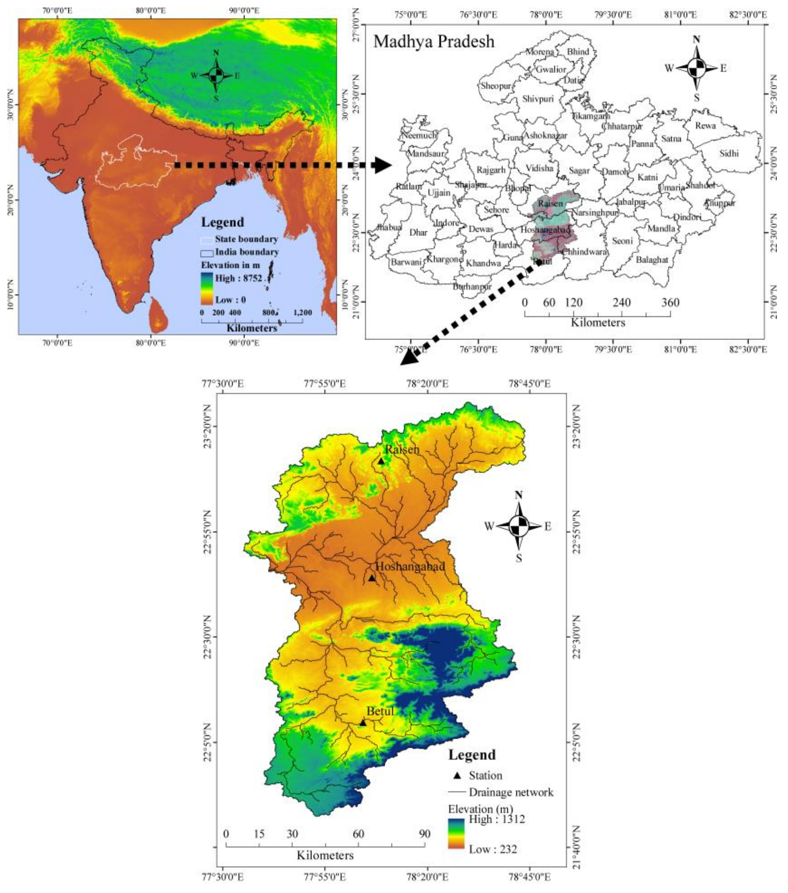
2. Study Area
3. Data and Methodology
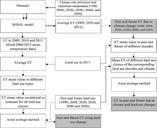
- (i)
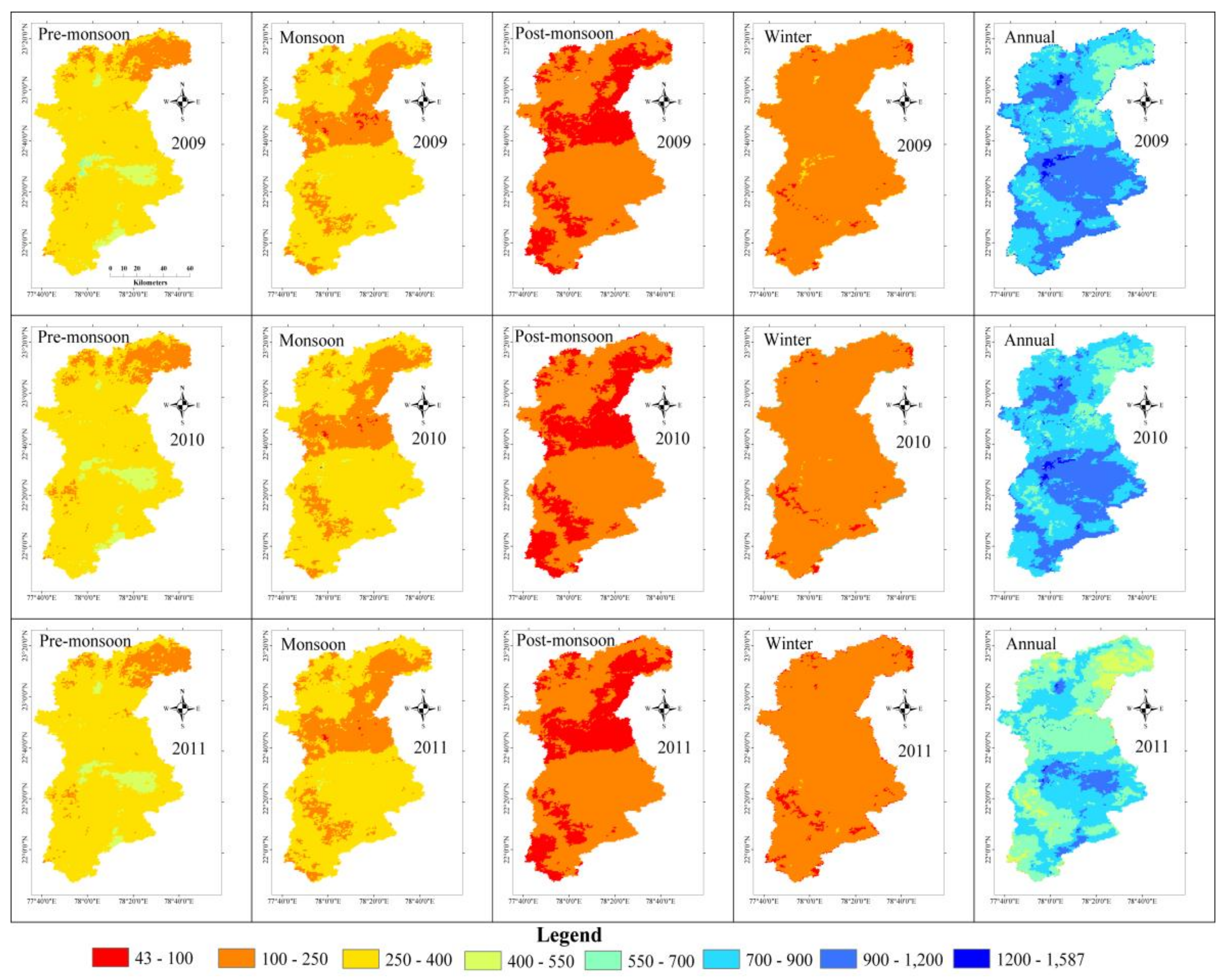
- ET was generated using SEBAL with 3 years (2009–2011) of MODIS data, and an average of three years of data was considered to reduce the uncertainty in actual ET estimation. Cloud-free images of 8-day composite were used to give the seasonal (premonsoon, monsoon, postmonsoon, and winter) and annual ET of three years.
- (ii)
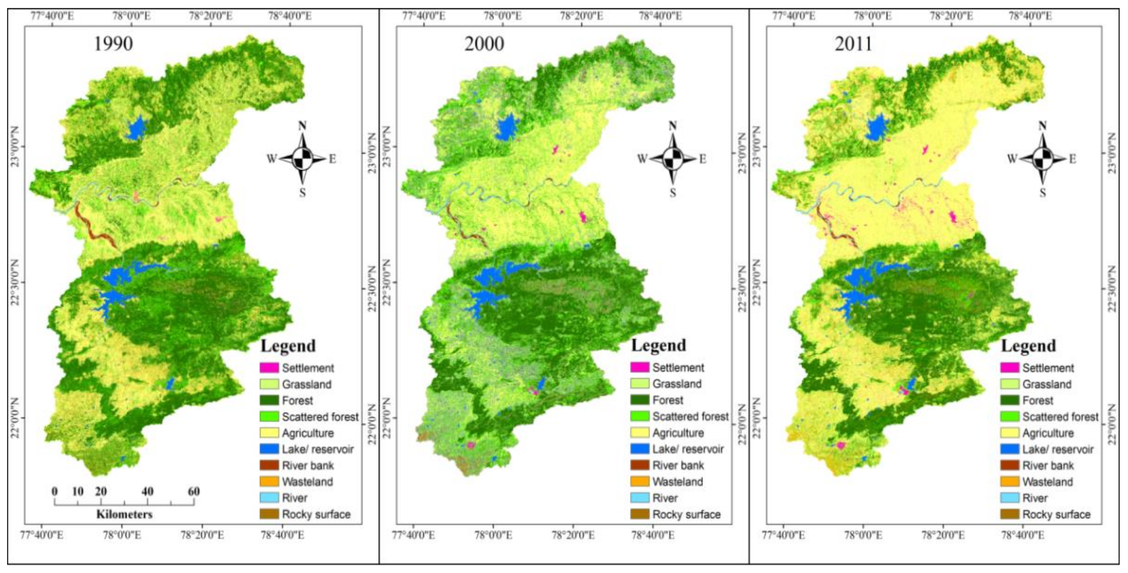
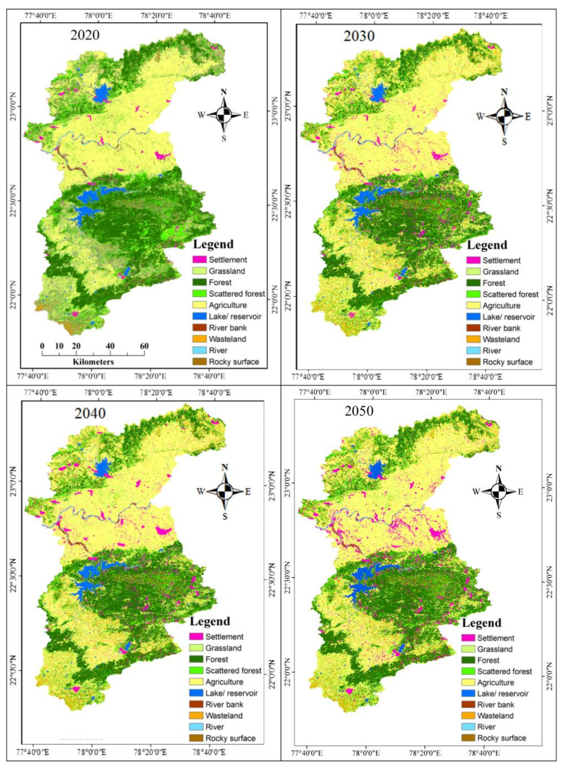
- Land use classification into 10 classes was done using Maximum Likelihood Classification techniques with three images from 1990, 2000, and 2011. The land use change prediction of 2020, 2030, 2040, and 2050 was done with the Markov Chain model using data from 1990, 2000, and 2011.
- (iii)
- To estimate climate change, RCP data from two scenarios (4.5 and 8.5) were used. Change in the minimum and maximum temperatures in the past and future was estimated by taking an average of 10 years of data. Climate change assessment of different decades spans the 1990s (average of 1986–1995), 2000s (1996–2005), 2011s (2006–2015), 2020s (2016–2025), 2030s (2026–2035), 2040s (2036–2045), and 2050s (2046–2055).
- (iv)
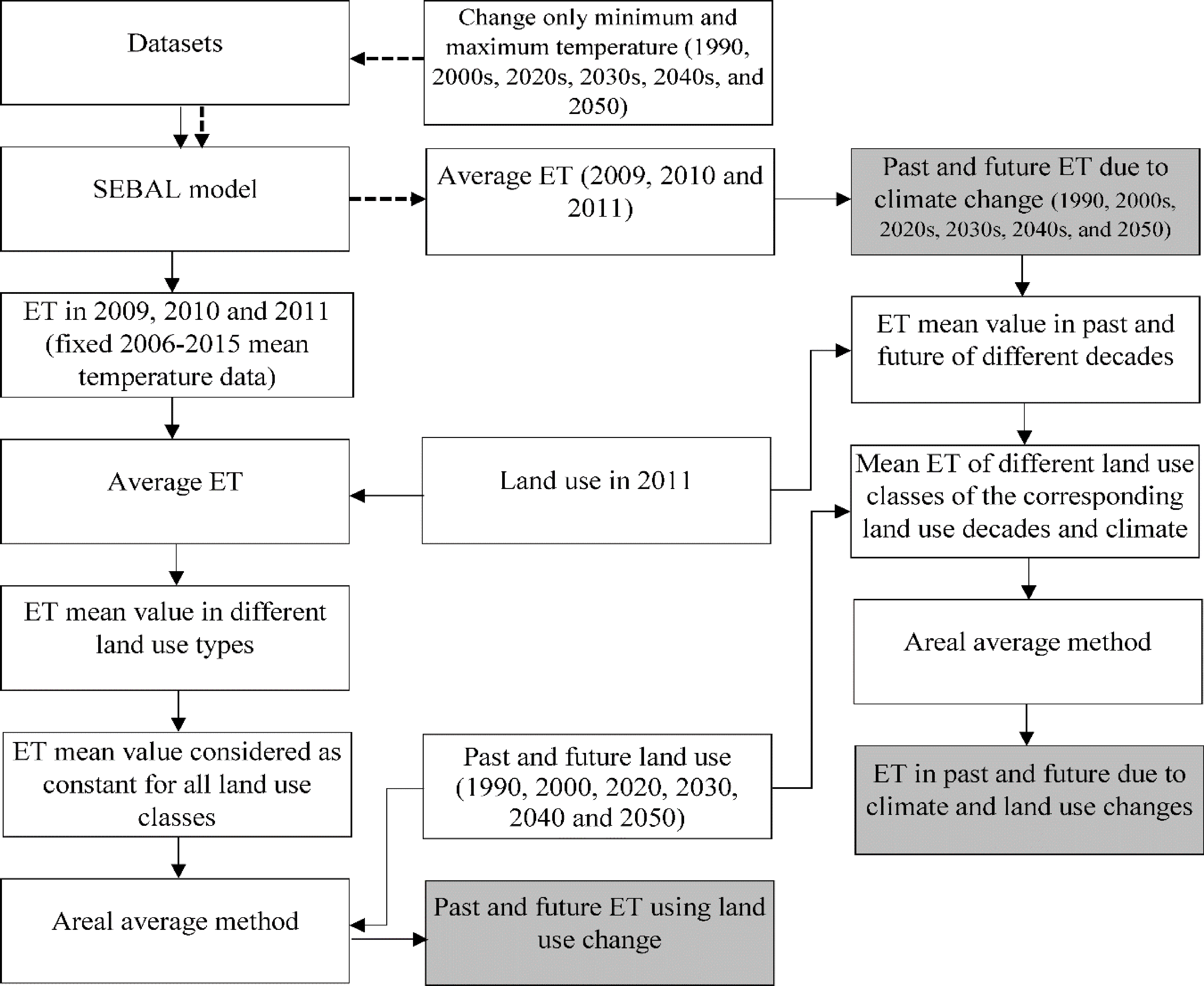
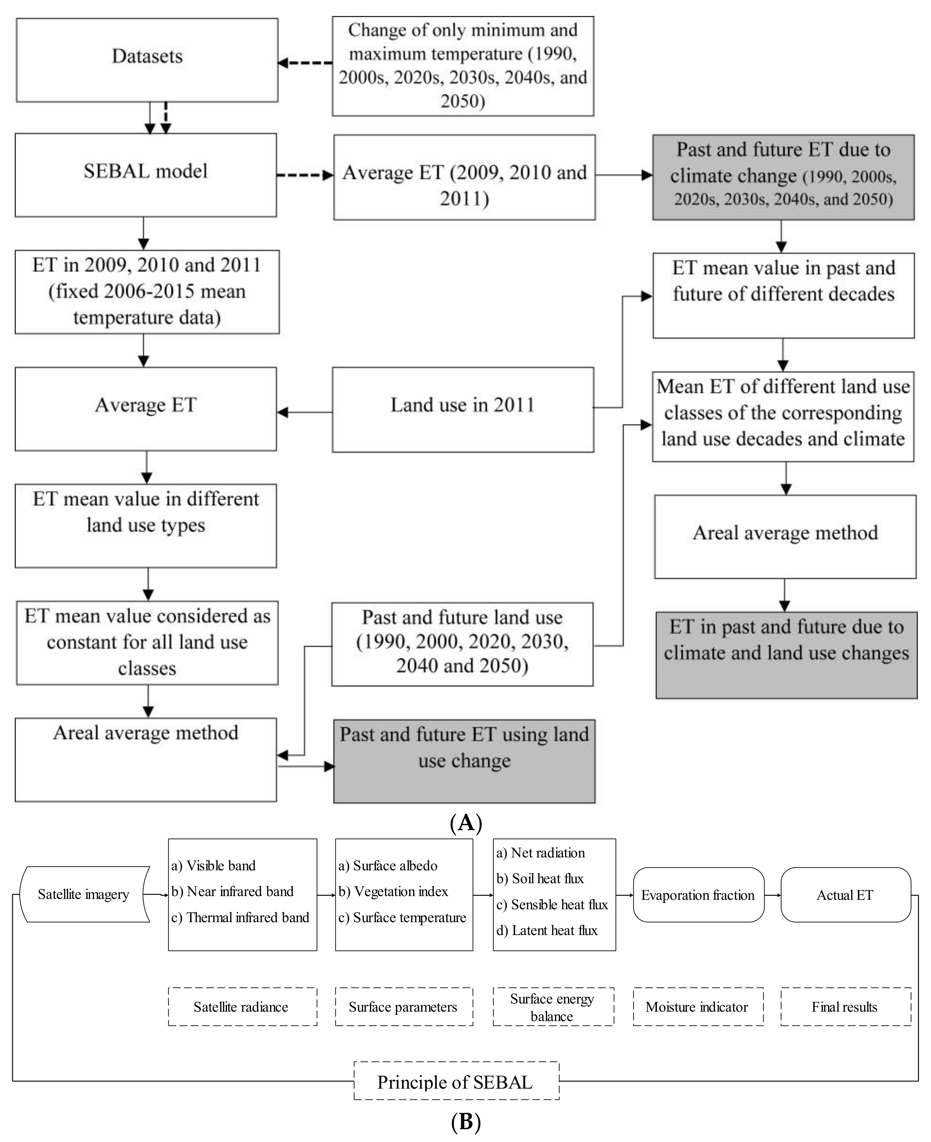
- The mean ET for 10 different land use classes was estimated from the 3 years’ mean ET of different seasons (2009–2011). The mean ET thus obtained was taken as a constant for different land use classes. The impact of land use change on ET was done by taking mean ET of 10 land use classes as constants on the basis of 2011 land use, and estimating ET of the past (1990, 2000) and future (2020, 2030, 2040, and 2050) with respect to changed land use by areal average method.
- (v)
- The impact of climate change on ET in all the years was estimated by changing the minimum and maximum temperature of the corresponding years (1990s, 2000s, 2020s, 2030s, 2040s, and 2050s) in the SEBAL model. All other parameters were kept constant (of the years 2009–2011). ET changes due to the effect of climate change for each decade were obtained by averaging ET of three years (2009–2011).
- (vi)
- (The mean ET of 10 land use classes of each decade (of climate years) was estimated on the basis of 2011 land use. Estimation of the combined impact of land use and climate change on future ET was done by using these mean ET (1990s, 2000s, 2011s, 2020s, 2030s, 2040s, 2050s) with the corresponding land use areas (1990, 2000, 2011, 2020, 2030, 2040, 2050) by areal average method (Figure 2A).
3.1. SEBAL Model (Actual ET)
3.2. Land Use Classification and Future Projection
3.3. Climate Change Prediction
4. Results
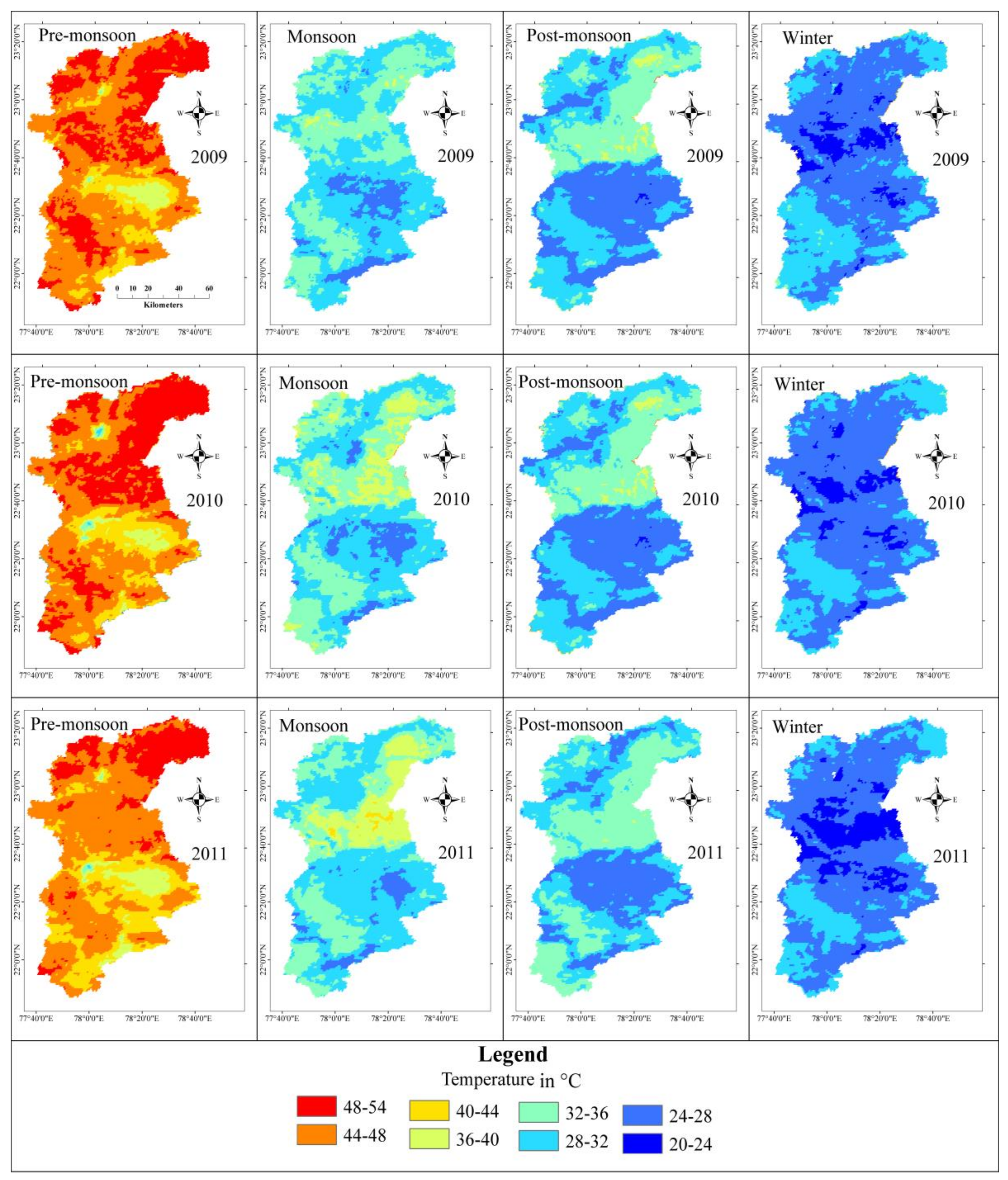
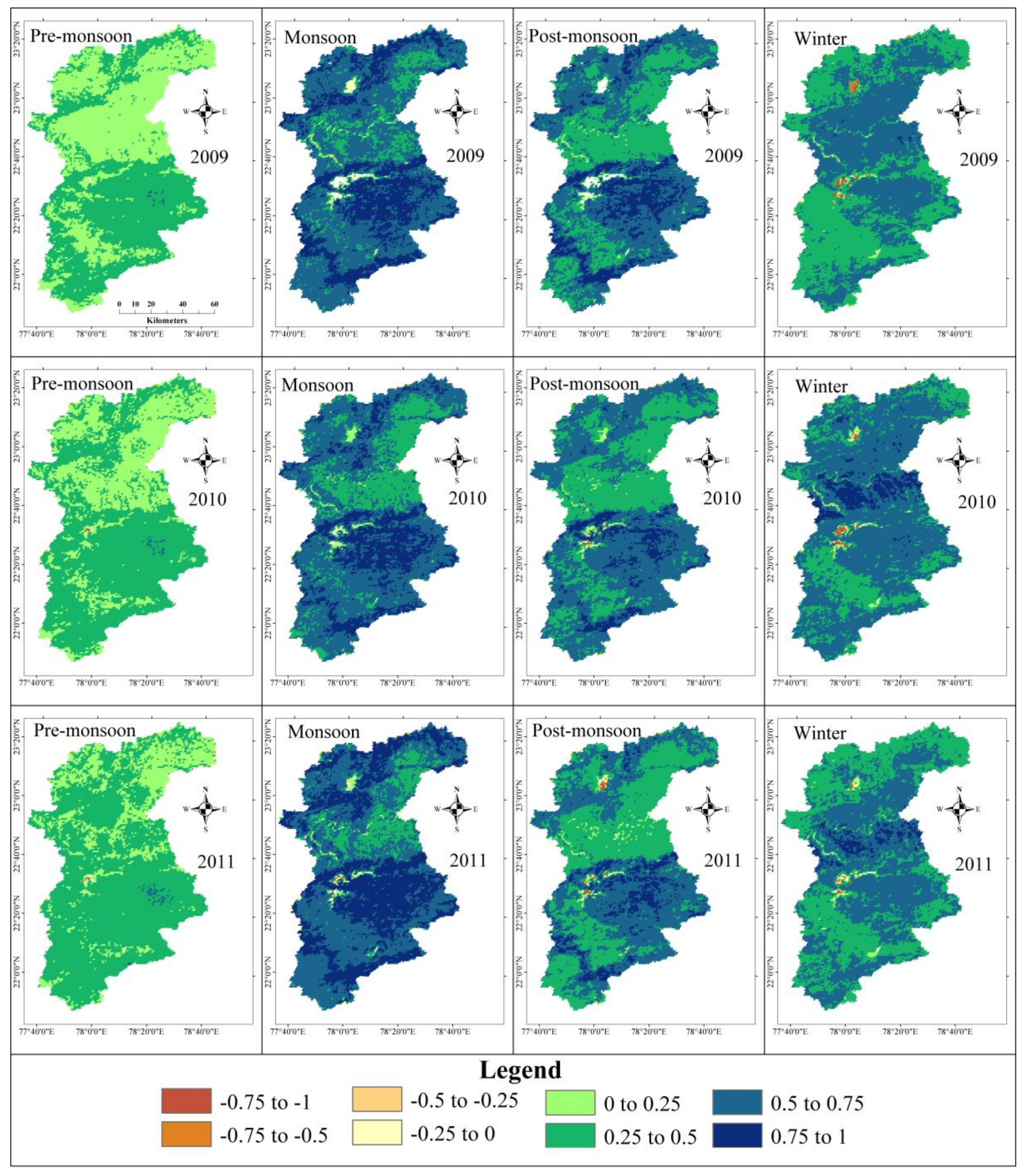
4.1. Seasonal and Annual Land Surface Temperature (LST) and Normalized Difference Vegetation Index (NDVI)
4.2. Seasonal and Annual Actual ET of 2009–2011
4.3. Future Scenarios of Land Use Change
Seasonal Mean ET for Different Land Use
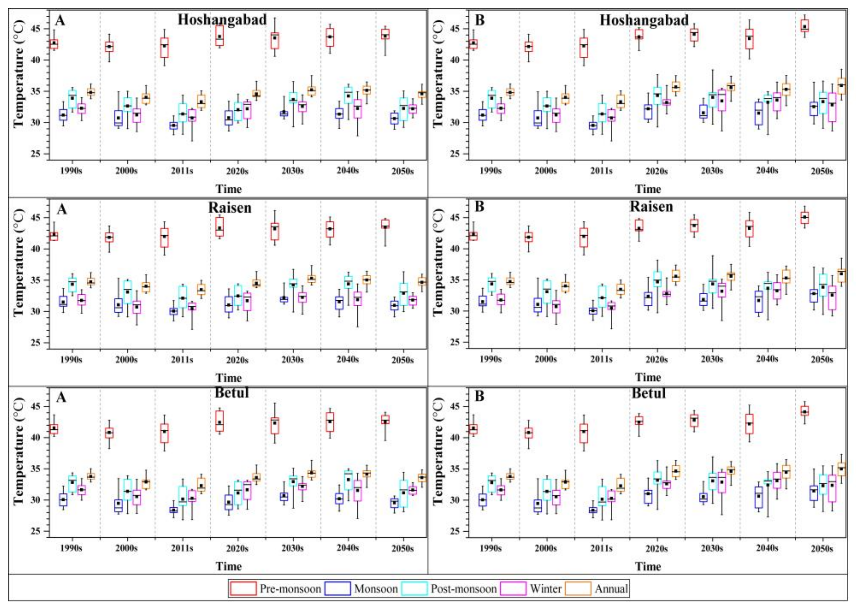
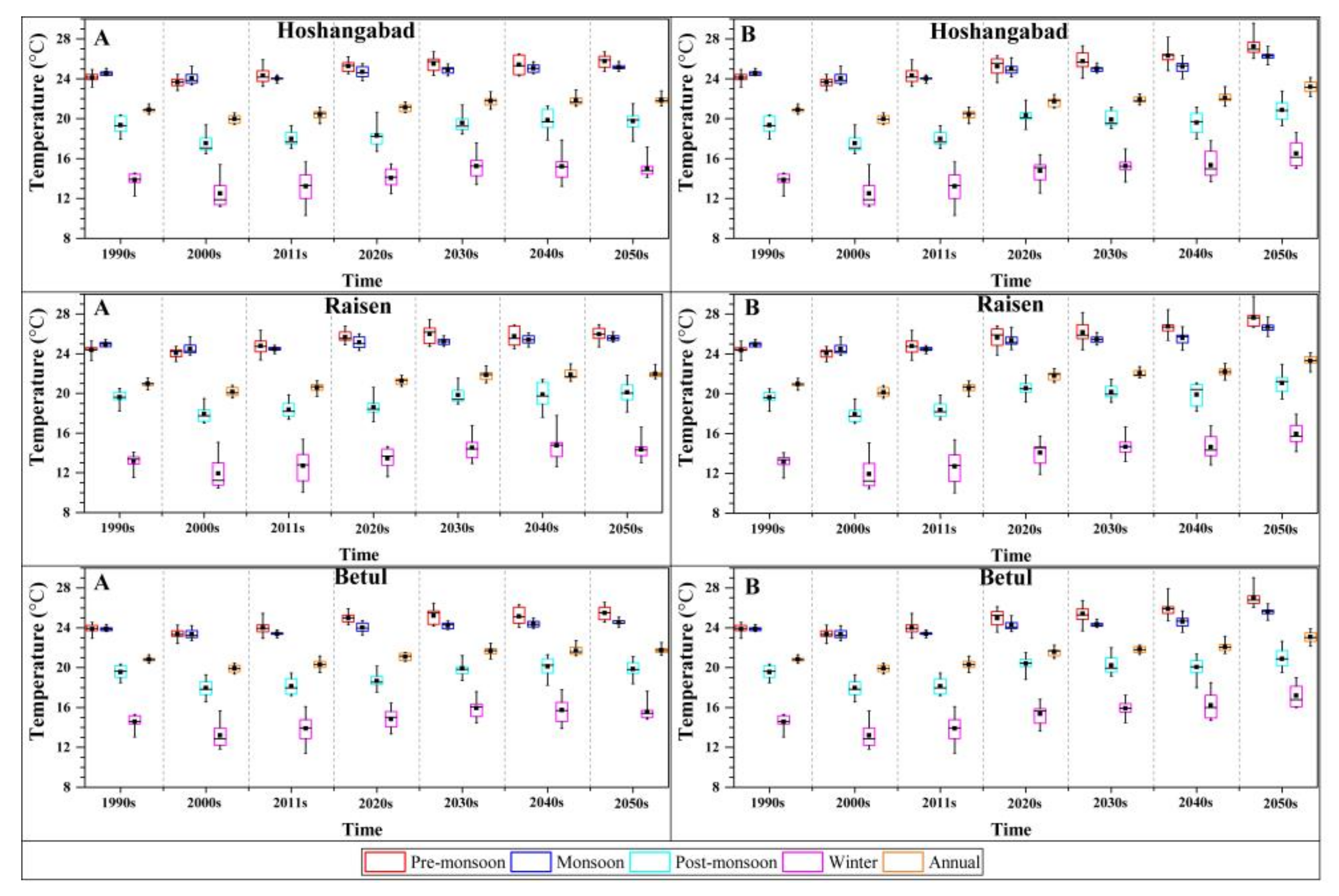
4.4. Future Climate Change
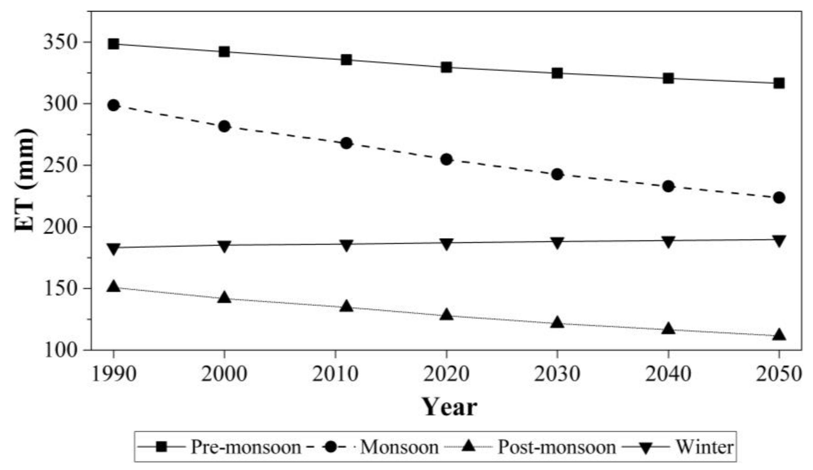
4.5. Impact of Future Climate and Land Use Changes on ET
4.5.1. Future Change of Seasonal and Annual ET Due to Land Use Change
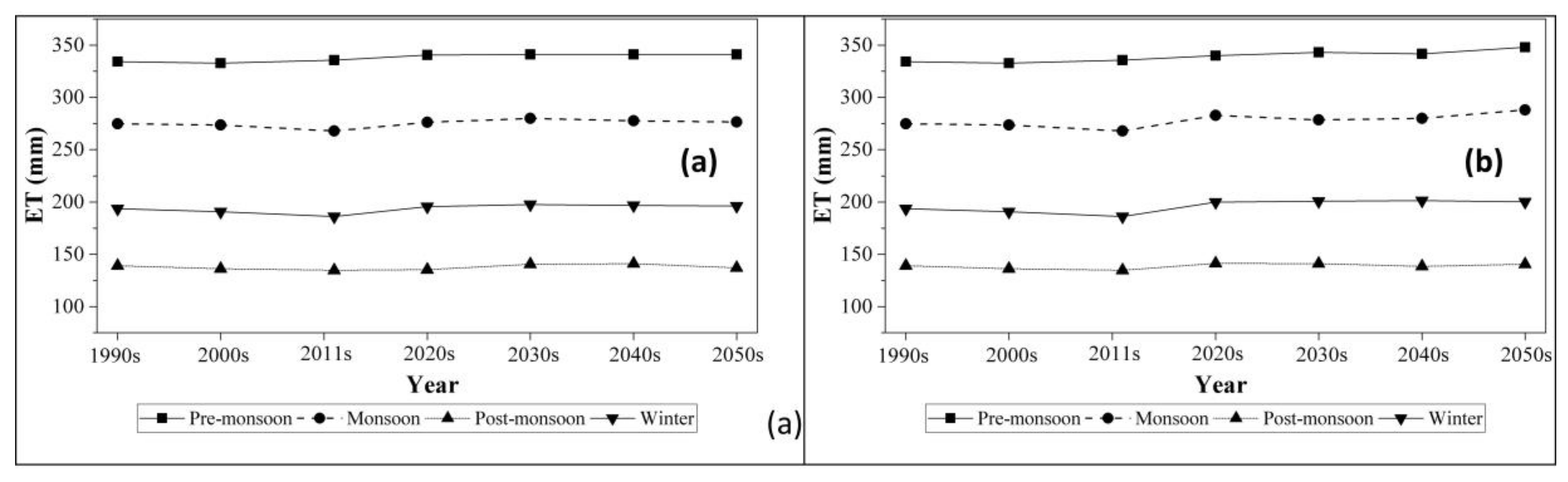
4.5.2. Future Change of Seasonal and Annual ET Due to Climate Change
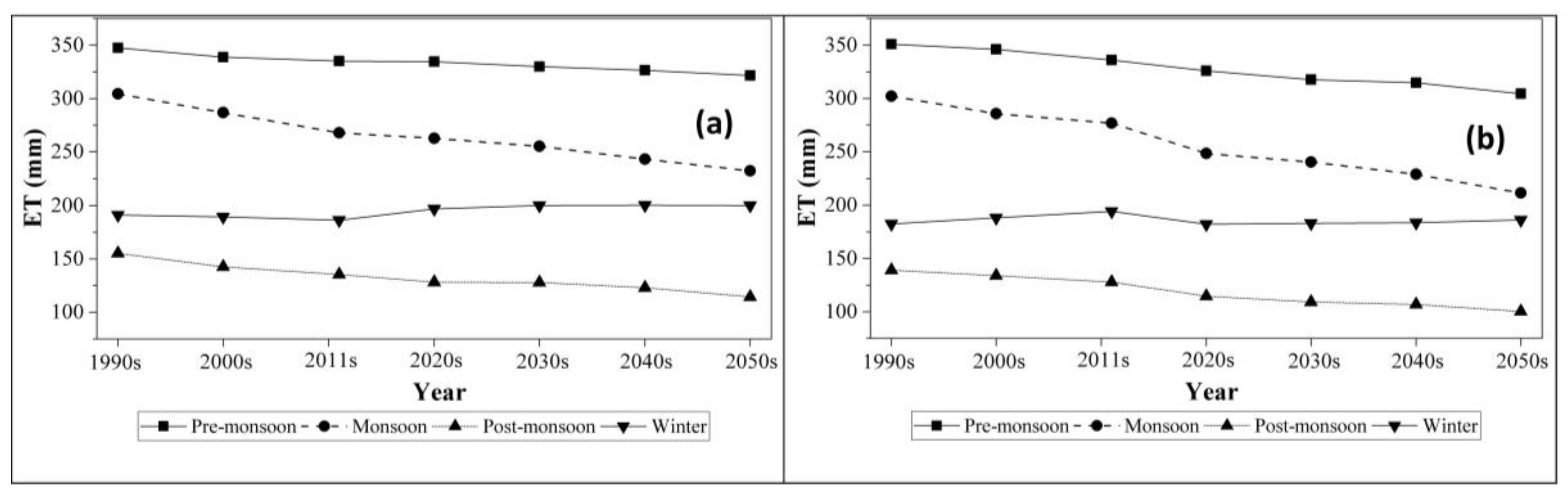
4.5.3. Future Change of Seasonal and Annual ET Due to Climate and Land Use Changes
5. Discussion and Conclusions
Supplementary Materials
Acknowledgments
Author Contributions
Conflicts of Interest
References
- Bouwer, L.M.; Biggs, T.W.; Aerts, J.C. Estimates of spatial variation in evaporation using satellite-derived surface temperature and a water balance model. Hydrol. Process. 2008, 22, 670–682. [Google Scholar] [CrossRef]
- Bergez, J.-E.; Garcia, F.; Lapasse, L. A hierarchical partitioning method for optimizing irrigation strategies. Agric. Syst. 2004, 80, 235–253. [Google Scholar] [CrossRef]
- Gowda, P.H.; Chavez, J.L.; Colaizzi, P.D.; Evett, S.R.; Howell, T.A.; Tolk, J.A. ET mapping for agricultural water management: Present status and challenges. Irrig. Sci. 2008, 26, 223–237. [Google Scholar] [CrossRef]
- Intergovernmental Panel on Climate Change (IPCC). Working Group II: Impacts, Adaptation and Vulnerability. 2000. Available online: http://www.ipcc.ch/ipccreports/tar/wg2/index.php?idp=29 (accessed on 2 April 2018).
- Shukla, J.; Mintz, Y. Influence of land-surface evapotranspiration on the earth’s climate. Science 1982, 215, 1498–1501. [Google Scholar] [CrossRef] [PubMed]
- Seneviratne, S.I.; Koster, R.D.; Guo, Z.; Dirmeyer, P.A.; Kowalczyk, E.; Lawrence, D.; Liu, P.; Mocko, D.; Lu, C.H.; Oleson, K.W.; et al. Soil moisture memory in AGCM simulations: Analysis of global land–atmosphere coupling experiment (GLACE) data. J. Hydrometeorol. 2006, 7, 1090–1112. [Google Scholar] [CrossRef]
- Vicente-Serrano, S.M.; Azorin-Molina, C.; Sanchez-Lorenzo, A.; Revuelto, J.; López-Moreno, J.I.; González-Hidalgo, J.C.; Moran-Tejeda, E.; Espejo, F. Reference evapotranspiration variability and trends in Spain, 1961–2011. Glob. Planet. Chang. 2014, 121, 26–40. [Google Scholar] [CrossRef]
- Wiesner, C.J. Climate, Irrigation and Agriculture; Angus and Robertson: Sydney, Australia, 1970. [Google Scholar]
- Hassan, Q.K.; Bourque, C.P.-A.; Meng, F.-R.; Cox, R.M. A wetness index using terrain-corrected surface temperature and normalized difference vegetation index derived from standard MODIS products: An evaluation of its use in a humid forest-dominated region of eastern Canada. Sensors 2007, 7, 2028–2048. [Google Scholar] [CrossRef] [PubMed]
- King, D.A.; Bachelet, D.M.; Symstad, A.J.; Ferschweiler, K.; Hobbins, M. Estimation of potential evapotranspiration from extraterrestrial radiation, air temperature and humidity to assess future climate change effects on the vegetation of the Northern Great Plains, USA. Ecol. Model. 2015, 297, 86–97. [Google Scholar] [CrossRef]
- Stroeve, J.C.; Box, J.E.; Haran, T. Evaluation of the MODIS (MOD10A1) daily snow albedo product over the Greenland ice sheet. Remote Sens. Environ. 2006, 105, 155–171. [Google Scholar] [CrossRef]
- Huo, Z.; Dai, X.; Feng, S.; Kang, S.; Huang, G. Effect of climate change on reference evapotranspiration and aridity index in arid region of China. J. Hydrol. 2013, 492, 24–34. [Google Scholar] [CrossRef]
- Rahimi, S.; Sefidkouhi, M.A.G.; Raeini-Sarjaz, M.; Valipour, M. Estimation of actual evapotranspiration by using MODIS images (a case study: Tajan catchment). Arch. Agron. Soil Sci. 2015, 61, 695–709. [Google Scholar] [CrossRef]
- Tang, R.; Li, Z.-L.; Sun, X. Temporal upscaling of instantaneous evapotranspiration: An intercomparison of four methods using eddy covariance measurements and MODIS data. Remote Sens. Environ. 2013, 138, 102–118. [Google Scholar] [CrossRef]
- Wild, M.; Folini, D.; Schär, C.; Loeb, N.; Dutton, E.G.; König-Langlo, G. The global energy balance from a surface perspective. Clim. Dyn. 2013, 40, 3107–3134. [Google Scholar] [CrossRef]
- Droogers, P.; Bastiaanssen, W. Irrigation performance using hydrological and remote sensing modeling. J. Irrig. Drain. Eng. 2002, 128, 11–18. [Google Scholar] [CrossRef]
- Bastiaanssen, W.; Noordman, E.; Pelgrum, H.; Davids, G.; Thoreson, B.; Allen, R. Sebal model with remotely sensed data to improve water-resources management under actual field conditions. J. Irrig. Drain. Eng. 2005, 131, 85–93. [Google Scholar] [CrossRef]
- Allen, R.G.; Tasumi, M.; Trezza, R. Satellite-based energy balance for mapping evapotranspiration with internalized calibration (metric)—Model. J. Irrig. Drain. Eng. 2007, 133, 380–394. [Google Scholar] [CrossRef]
- Laymon, C.; Quattrochi, D.; Malek, E.; Hipps, L.; Boettinger, J.; McCurdy, G. Remotely-sensed regional-scale evapotranspiration of a semi-arid Great Basin Desert and its relationship to geomorphology, soils, and vegetation. Geomorphology 1998, 21, 329–349. [Google Scholar] [CrossRef]
- Morse, A.; Tasumi, M.; Allen, R.G.; Kramber, W.J. Application of the SEBAL Methodology for Estimating Consumptive Use of Water and Streamflow Depletion in the Bear River Basin of Idaho through Remote Sensing; Idaho Department of Water Resources: Boise, ID, USA; University of Idaho, ID, USA, 2000. [Google Scholar]
- Batra, N.; Islam, S.; Venturini, V.; Bisht, G.; Jiang, L. Estimation and comparison of evapotranspiration from MODIS and AVHRR sensors for clear sky days over the southern great plains. Remote Sens. Environ. 2006, 103, 1–15. [Google Scholar] [CrossRef]
- McCabe, M.F.; Wood, E.F. Scale influences on the remote estimation of evapotranspiration using multiple satellite sensors. Remote Sens. Environ. 2006, 105, 271–285. [Google Scholar] [CrossRef]
- Zhang, X.; Sun, R.; Zhang, B.; Tong, Q. Land cover classification of the north China plain using MODIS-EVI time series. ISPRS J. Photogramm. Remote Sens. 2008, 63, 476–484. [Google Scholar] [CrossRef]
- Kiptala, J.; Mohamed, Y.; Mul, M.L.; Zaag, P. Mapping evapotranspiration trends using MODIS and SEBAL model in a data-scarce and heterogeneous landscape in eastern Africa. Water Resour. Res. 2013, 49, 8495–8510. [Google Scholar] [CrossRef]
- Sun, Z.; Gebremichael, M.; Ardö, J.; Nickless, A.; Caquet, B.; Merboldh, L.; Kutschi, W. Estimation of daily evapotranspiration over Africa using MODIS/TERRA and SEVIRI/MSG data. Atmos. Res. 2012, 112, 35–44. [Google Scholar] [CrossRef]
- Cammalleri, C.; Anderson, M.; Gao, F.; Hain, C.; Kustas, W. A data fusion approach for mapping daily evapotranspiration at the field scale. Water Resour. Res. 2013, 49, 4672–4686. [Google Scholar] [CrossRef]
- Cammalleri, C.; Anderson, M.; Gao, F.; Hain, C.; Kustas, W. Mapping daily evapotranspiration at field scales over rainfed and irrigated agricultural areas using remote sensing data fusion. Agric. For. Meteorol. 2014, 186, 1–11. [Google Scholar] [CrossRef]
- Bastiaanssen, W.G.; Menenti, M.; Feddes, R.; Holtslag, A. A remote sensing surface energy balance algorithm for land (SEBAL). 1. Formulation. J. Hydrol. 1998, 212, 198–212. [Google Scholar] [CrossRef]
- Bastiaanssen, W.G.; Pelgrum, H.; Wang, J.; Ma, Y.; Moreno, J.; Roerink, G.; Van der Wal, T. A remote sensing surface energy balance algorithm for land (SEBAL): Part 2: Validation. J. Hydrol. 1998, 212, 213–229. [Google Scholar] [CrossRef]
- Sun, Z.; Wei, B.; Su, W.; Shen, W.; Wang, C.; You, D.; Liu, Z. Evapotranspiration estimation based on the SEBAL model in the Nansi lake wetland of China. Math. Comput. Model. 2011, 54, 1086–1092. [Google Scholar] [CrossRef]
- Du, J.; Song, K.; Wang, Z.; Zhang, B.; Liu, D. Evapotranspiration estimation based on MODIS products and surface energy balance algorithms for land (SEBAL) model in Sanjiang plain, northeast china. Chin. Geogr. Sci. 2013, 23, 73–91. [Google Scholar] [CrossRef]
- Bastiaanssen, W.; Pelgrum, H.; Soppe, R.; Allen, R.; Thoreson, B.; de C. Teixeira, A. Thermal-infrared technology for local and regional scale irrigation analyses in horticultural systems. ActaHortic 2008, 792, 33–46. [Google Scholar]
- Papadavid, G.; Hadjimitsis, D.G.; Toulios, L.; Michaelides, S. A modified sebal modeling approach for estimating crop evapotranspiration in semi-arid conditions. Water Resour. Manag. 2013, 27, 3493–3506. [Google Scholar] [CrossRef]
- Bashir, M.; Hata, T.; Tanakamaru, H.; Abdelhadi, A.; Tada, A. Satellite-based energy balance model to estimate seasonal evapotranspiration for irrigated sorghum: A case study from the Gezira scheme, Sudan. Hydrol. Earth Syst. Sci. 2008, 12, 1129–1139. [Google Scholar] [CrossRef]
- Abrishamkar, M.; Ahmadi, A. Evapotranspiration estimation using remote sensing technology based on SEBAL algorithm. Iran. J. Sci. Technol. Trans. Civ. Eng. 2017, 41, 65–76. [Google Scholar] [CrossRef]
- Ahmad, M.-D.; Biggs, T.; Turral, H.; Scott, C.A. Application of SEBAL approach and modis time-series to map vegetation water use patterns in the data scarce Krishna river basin of India. Water Sci. Technol. 2006, 53, 83–90. [Google Scholar] [CrossRef] [PubMed]
- Bala, A.; Rawat, K.S.; Misra, A.K.; Srivastava, A. Assessment and validation of evapotranspiration using SEBAL algorithm and lysimeter data of IARI agricultural farm, India. Geocarto Int. 2016, 31, 739–764. [Google Scholar] [CrossRef]
- Parmar, H.; Gontia, N. Irrigation water management modeling in canal command using remote sensing. Ann. Arid Zone 2016, 55, 89–99. [Google Scholar]
- Jana, C.; Rawat, M.; Sena, D.R.; Alam, N.M.; Mandal, U.; Kaushal, R.; Mishra, P.K. Application of SEBAL model to estimate Evapotranspiration in Doon Valley, India. Indian J. Soil Conserv. 2016, 44, 191–197. [Google Scholar]
- Cai, X.; Sharma, B.R. Integrating remote sensing, census and weather data for an assessment of rice yield, water consumption and water productivity in the Indo-Gangetic river basin. Agric. Water Manag. 2010, 97, 309–316. [Google Scholar] [CrossRef]
- Mahmoud, S.H.; Alazba, A. A coupled remote sensing and the surface energy balance based algorithms to estimate actual evapotranspiration over the western and southern regions of Saudi Arabia. J. Asian Earth Sci. 2016, 124, 269–283. [Google Scholar] [CrossRef]
- Bastiaanssen, W. SEBAL-based sensible and latent heat fluxes in the irrigated Gediz basin, turkey. J. Hydrol. 2000, 229, 87–100. [Google Scholar] [CrossRef]
- Timmermans, W.J.; Kustas, W.P.; Anderson, M.C.; French, A.N. An intercomparison of the surface energy balance algorithm for land (SEBAL) and the two-source energy balance (TSEB) modeling schemes. Remote Sens. Environ. 2007, 108, 369–384. [Google Scholar] [CrossRef]
- Minacapilli, M.; Agnese, C.; Blanda, F.; Cammalleri, C.; Ciraolo, G.; D’Urso, G.; Iovino, M.; Pumo, D.; Provenzano, G.; Rallo, G. Estimation of actual evapotranspiration of Mediterranean perennial crops by means of remote-sensing based surface energy balance models. Hydrol. Earth Syst. Sci. 2009, 13, 1061–1074. [Google Scholar] [CrossRef] [Green Version]
- Yang, J.-Y.; Mei, X.-R.; Huo, Z.-G.; Yan, C.-R.; Hui, J.; Zhao, F.-H.; Qin, L. Water consumption in summer maize and winter wheat cropping system based on SEBAL model in Huang-Huai-Hai plain, China. J. Integr. Agric. 2015, 14, 2065–2076. [Google Scholar] [CrossRef]
- Wu, B.; Zhu, W.; Yan, N.; Feng, X.; Xing, Q.; Zhuang, Q. An improved method for deriving daily evapotranspiration estimates from satellite estimates on cloud-free days. IEEE J. Sel. Top. Appl. Earth Obs. Remote Sens. 2016, 9, 1323–1330. [Google Scholar] [CrossRef]
- Luo, T.; Jutla, A.; Islam, S. Evapotranspiration estimation over agricultural plains using MODIS data for all sky conditions. Int. J. Remote Sens. 2015, 36, 1235–1252. [Google Scholar] [CrossRef]
- Steele, D.D.; Thoreson, B.P.; Hopkins, D.G.; Clark, B.A.; Tuscherer, S.R.; Gautam, R. Spatial mapping of evapotranspiration over Devils lake basin with SEBAL: Application to flood mitigation via irrigation of agricultural crops. Irrig. Sci. 2015, 33, 15–29. [Google Scholar] [CrossRef]
- Senay, G.B.; Friedrichs, M.; Singh, R.K.; Velpuri, N.M. Evaluating landsat 8 evapotranspiration for water use mapping in the colorado river basin. Remote Sens. Environ. 2016, 185, 171–185. [Google Scholar] [CrossRef]
- Jiménez-Bello, M.Á.; Castel, J.R.; Testi, L.; Intrigliolo, D.S. Assessment of a remote sensing energy balance methodology (SEBAL) using different interpolation methods to determine evapotranspiration in a citrus orchard. IEEE J. Sel. Top. Appl. Earth Obs. Remote Sens. 2015, 8, 1465–1477. [Google Scholar] [CrossRef]
- Bhattarai, N.; Shaw, S.B.; Quackenbush, L.J.; Im, J.; Niraula, R. Evaluating five remote sensing based single-source surface energy balance models for estimating daily evapotranspiration in a humid subtropical climate. Int. J. Appl. Earth Obs. Geoinform. 2016, 49, 75–86. [Google Scholar] [CrossRef]
- Tang, R.; Li, Z.-L. Evaluation of two end-member-based models for regional land surface evapotranspiration estimation from MODIS data. Agric. For. Meteorol. 2015, 202, 69–82. [Google Scholar] [CrossRef]
- Lian, J.; Huang, M. Comparison of three remote sensing based models to estimate evapotranspiration in an oasis-desert region. Agric. Water Manag. 2016, 165, 153–162. [Google Scholar] [CrossRef]
- Sharma, V.; Kilic, A.; Irmak, S. Impact of scale/resolution on evapotranspiration from Landsat and MODIS images. Water Resour. Res. 2016, 52, 1800–1819. [Google Scholar] [CrossRef]
- Wang, Y.Q.; Xiong, Y.J.; Qiu, G.Y.; Zhang, Q.T. Is scale really a challenge in evapotranspiration estimation? A multi-scale study in the Heihe oasis using thermal remote sensing and the three-temperature model. Agric. For. Meteorol. 2016, 230, 128–141. [Google Scholar] [CrossRef]
- Zheng, C.; Wang, Q.; Li, P. Coupling SEBAL with a new radiation module and MODIS products for better estimation of evapotranspiration. Hydrol. Sci. J. 2016, 61, 1535–1547. [Google Scholar] [CrossRef]
- Liaqat, U.W.; Choi, M. Accuracy comparison of remotely sensed evapotranspiration products and their associated water stress footprints under different land cover types in Korean peninsula. J. Clean. Prod. 2016, 155, 93–104. [Google Scholar] [CrossRef]
- Alidoost, F.; Sharifi, M.A.; Stein, A. Region-and pixel-based image fusion for disaggregation of actual evapotranspiration. Int. J. Image Data Fusion 2015, 6, 216–231. [Google Scholar] [CrossRef]
- Allen, R.G.; Pereira, L.S.; Raes, D.; Smith, M. Crop Evapotranspiration-Guidelines for Computing Crop Water Requirements-FAO Irrigation and Drainage Paper 56; FAO: Rome, Italy, 1998; Volume 300, p. D05109. [Google Scholar]
- Bastiaanssen, W.G.M. Regionalization of surface flux densities and moisture indicators in composite terrain. In a Remote Sensing Approach under Clear Skies in Mediterranean Climates. 1995. Available online: http://library.wur.nl/WebQuery/wda/918192(accessed on 10 May 2012).
- Goetz, S. Multi-sensor analysis of NDVI, surface temperature and biophysical variables at a mixed grassland site. Int. J. Remote Sens. 1997, 18, 71–94. [Google Scholar] [CrossRef]
- Allen, R.; Tasumi, M.; Trezza, R.; Waters, R.; Bastiaanssen, W. Sebal (surface energy balance algorithms for land). In Advance Training and Users Manual–Idaho Implementation, Version. 2002; Volume 1, 97. Available online: https://www.researchgate.net/file.PostFileLoader.html?id=5635f25060614b180d8b4567&assetKey=AS%3A290936253894656%401446376016229(accessed on 8 May 2012).
- Wu, Q.; Li, H.-Q.; Wang, R.-S.; Paulussen, J.; He, Y.; Wang, M.; Wang, B.-H.; Wang, Z. Monitoring and predicting land use change in Beijing using remote sensing and GIS. Landsc. Urban Plan. 2006, 78, 322–333. [Google Scholar] [CrossRef]
- Mukhopadhyay, A.; Mondal, A.; Mukherjee, S.; Khatua, D.; Ghosh, S.; Mitra, D.; Ghosh, T. Forest cover change prediction using hybrid methodology of geoinformatics and markov chain model: A case study on sub-himalayan town Gangtok, India. J. Earth Syst. Sci. 2014, 123, 1349–1360. [Google Scholar] [CrossRef]
- Mondal, A.; Khare, D.; Kundu, S.; Mishra, P.; Meena, P. Landuse Change Prediction and Its Impact on surface Run-Off Using Fuzzy C-Mean, Markov Chain and Curve Number Methods. In Proceedings of the Third International Conference on Soft Computing for Problem; Springer: Berlin, Germany, 2014; pp. 365–376. Available online: https://doi.org/10.1007/978-81-322-1768-8_33 (accessed on 5 March 2014).
- Chen, C.-F.; Son, N.-T.; Chang, N.-B.; Chen, C.-R.; Chang, L.-Y.; Valdez, M.; Centeno, G.; Thompson, C.A.; Aceituno, J.L. Multi-decadal mangrove forest change detection and prediction in Honduras, central America, with Landsat imagery and a Markov chain model. Remote Sens. 2013, 5, 6408–6426. [Google Scholar] [CrossRef]
- Alqurashi, A.F.; Kumar, L.; Sinha, P. Urban land cover change modelling using time-series satellite images: A case study of urban growth in five cities of Saudi Arabia. Remote Sens. 2016, 8, 838. [Google Scholar] [CrossRef]
- Athmania, D.; Achour, H. External validation of the Aster GDEM2, gmted2010 and CGIAR-CSI-SRTM v4. 1 free access digital elevation models (DEMs) in Tunisia and Algeria. Remote Sens. 2014, 6, 4600–4620. [Google Scholar] [CrossRef]
- Scott, A.J.; Symons, M.J. Clustering methods based on likelihood ratio criteria. Biometrics 1971, 27, 387–397. [Google Scholar] [CrossRef]
- Wang, G.; He, G.; Liu, J. A New Classification Method for High Spatial Resolution Remote Sensing Image Based on Mapping Mechanism. In Proceedings of the International Conference on Geographic Object-Based Image Analysis (GEOBIA’12), Rio de Janeiro, Brazil, 7–9 May 2012; pp. 186–190. [Google Scholar]
- Weng, Q. Land use change analysis in the Zhujiang delta of china using satellite remote sensing, GIS and stochastic modelling. J. Environ. Manag. 2002, 64, 273–284. [Google Scholar] [CrossRef]
- Sanjay, J.; Krishnan, R.; Shrestha, A.B.; Rajbhandari, R.; Ren, G.Y. Downscaled climate change projections for the Hindu Kush Himalayan region using CORDEX South Asia regional climate models. Adv. Clim. Chang. Res. 2017, 8, 185–198. [Google Scholar] [CrossRef]
- Carlson, T.N.; Perry, E.M.; Schmugge, T.J. Remote estimation of soil moisture availability and fractional vegetation cover for agricultural fields. Agric. For. Meteorol. 1990, 52, 45–69. [Google Scholar] [CrossRef]
- Kalluri, S.N.; Townshend, J.R.; Doraiswamy, P. A simple single layer model to estimate transpiration from vegetation using multi-spectral and meteorological data. Int. J. Remote Sens. 1998, 19, 1037–1053. [Google Scholar] [CrossRef]
- Bindhu, V.M.; Narasimhan, B.; Sudheer, K.P. Development and verification of a non-linear disaggregation method (NL-DisTrad) to downscale MODIS land surface temperature to the spatial scale of Landsat thermal data to estimate evapotranspiration. Remote Sens. Environ. 2013, 135, 118–129. [Google Scholar] [CrossRef]
- Kumar, D.; Shekhar, S. Statistical analysis of land surface temperature–vegetation indexes relationship through thermal remote sensing. Ecotoxicol. Environ. Saf. 2015, 121, 39–44. [Google Scholar] [CrossRef] [PubMed]
- Guo, G.; Wu, Z.; Xiao, R.; Chen, Y.; Liu, X.; Zhang, X. Impacts of urban biophysical composition on land surface temperature in urban heat island clusters. Landsc. Urban Plan. 2015, 135, 1–10. [Google Scholar] [CrossRef]
- Tran, D.X.; Pla, F.; Latorre-Carmona, P.; Myint, S.W.; Caetano, M.; Kieu, H.V. Characterizing the relationship between land use land cover change and land surface temperature. ISPRS J. Photogramm. Remote Sens. 2017, 124, 119–132. [Google Scholar] [CrossRef]
- Landis, J.R.; Koch, G.G. The measurement of observer agreement for categorical data. Biometrics 1977, 33, 159–174. [Google Scholar] [CrossRef] [PubMed]
- Milich, L.; Weiss, E. Gac NDVI images: Relationship to rainfall and potential evaporation in the grazing lands of the Gourma (Northern Sahel) and in the croplands of the Niger-Nigeria border (Southern Sahel). Int. J. Remote Sens. 2000, 21, 261–280. [Google Scholar] [CrossRef]
- Papadavid, G.; Neocleous, D.; Kountios, G.; Markou, M.; Michailidis, A.; Ragkos, A.; Hadjimitsis, D. Using SEBAL to Investigate How Variations in Climate Impact on Crop Evapotranspiration. J. Imaging 2017, 3. [Google Scholar] [CrossRef]
- Kundu, S.; Khare, D.; Mondal, A. Individual and combined impacts of future climate and land use changes on the water balance. Ecol. Eng. 2017, 105, 42–57. [Google Scholar] [CrossRef]
- Yuan, X.; Bai, J.; Li, L.; Kurban, A.; De Maeyer, P. The dominant role of climate change in determining changes in evapotranspiration in Xinjiang, China from 2001 to 2012. PLoS ONE 2017, 12, e0183071. [Google Scholar] [CrossRef] [PubMed]


| Data Input | Source |
|---|---|
| Temperature (°C) | Indian Meteorological Department (IMD) |
| Relative Humidity (%) | |
| Wind speed (m/s) | |
| Incoming solar radiation (W/m2) | |
| Satellite Data Input (MODIS) | USGS |
| Temperature (°C) (Climate change analysis) | CORDEX |
| Sl. No. | Crops | Month of Sowing | Month of Harvesting |
|---|---|---|---|
| 1 | Wheat | November–December | February–March |
| 2 | Seasonal vegetables | June–July | September–Octorber |
| 3 | Seeds | November | February |
| 4 | Paddy | June–July | Octorber–November |
| 1990 | 2000 | 2011 | |||||||
| Sl. No. | Classes | Area (km2) | Area (%) | Area (km2) | Area (%) | Area (km2) | Area (%) | ||
| 1 | Settlement | 217.47 | 1.77 | 309.39 | 2.52 | 386.10 | 3.14 | ||
| 2 | Grassland | 1458.37 | 11.87 | 1367.25 | 11.12 | 1339.76 | 10.90 | ||
| 3 | Forest | 3664.04 | 29.81 | 3180.16 | 25.88 | 2726.56 | 22.19 | ||
| 4 | Scattered | 1270.51 | 10.34 | 1132.79 | 9.22 | 988.14 | 8.04 | ||
| 5 | Agriculture | 4106.21 | 33.41 | 5010.22 | 40.77 | 5643.67 | 45.92 | ||
| 6 | Lake/reservoir | 242.15 | 1.97 | 245.31 | 2.00 | 263.28 | 2.14 | ||
| 7 | River bank | 48.68 | 0.40 | 30.62 | 0.25 | 29.41 | 0.24 | ||
| 8 | Wasteland | 1138.95 | 9.27 | 855.23 | 6.96 | 741.85 | 6.04 | ||
| 9 | River | 56.37 | 0.46 | 65.62 | 0.53 | 63.08 | 0.51 | ||
| 10 | Rocky surface | 87.25 | 0.71 | 93.40 | 0.76 | 108.16 | 0.88 | ||
| Total | 12,290 | 100 | 12,290 | 100 | 12,290 | 100 | |||
| 2020 | 2030 | 2040 | 2050 | ||||||
| Sl No. | Classes | Area (km2) | Area (%) | Area (km2) | Area (%) | Area (km2) | Area (%) | Area (km2) | Area (%) |
| 1 | Settlement | 484.01 | 3.94 | 577.42 | 4.70 | 647.47 | 5.27 | 710.23 | 5.78 |
| 2 | Grassland | 1276.43 | 10.39 | 1221.12 | 9.94 | 1171.96 | 9.54 | 1125.65 | 9.16 |
| 3 | Forest | 2310.91 | 18.80 | 1948.36 | 15.85 | 1663.23 | 13.53 | 1391.62 | 11.32 |
| 4 | Scattered | 870.26 | 7.08 | 728.93 | 5.93 | 610.94 | 4.97 | 508.01 | 4.13 |
| 5 | Agriculture | 6275.32 | 51.06 | 6848.04 | 55.72 | 7305.22 | 59.44 | 7755.25 | 63.10 |
| 6 | Lake/reservoir | 270.51 | 2.20 | 284.03 | 2.31 | 293.25 | 2.39 | 303.50 | 2.47 |
| 7 | River bank | 21.80 | 0.18 | 16.88 | 0.14 | 12.58 | 0.10 | 10.17 | 0.08 |
| 8 | Wasteland | 598.54 | 4.87 | 462.12 | 3.76 | 357.66 | 2.91 | 245.20 | 2.00 |
| 9 | River | 64.23 | 0.52 | 70.38 | 0.57 | 72.22 | 0.59 | 70.23 | 0.57 |
| 10 | Rocky surface | 117.98 | 0.96 | 132.73 | 1.08 | 154.85 | 1.26 | 170.14 | 1.38 |
| Total | 12,290 | 100 | 12,290 | 100 | 12,289 | 100 | 12,290 | 100 | |
| Sl. No | Classes | Settlement | Grassland | Forest | Scattered Forest | Agriculture | Water Body | River Bank | Wasteland | Rocky Surface |
|---|---|---|---|---|---|---|---|---|---|---|
| 1 | Premonsoon | 294.71 | 300.02 | 467.77 | 331.86 | 282.39 | 647.07 | 346.33 | 228.52 | 189.11 |
| 2 | Monsoon | 183.20 | 257.42 | 429.03 | 389.59 | 159.62 | 497.96 | 183.41 | 315.17 | 175.88 |
| 3 | Postmonsoon | 78.18 | 116.05 | 220.31 | 199.62 | 80.52 | 263.27 | 99.68 | 161.70 | 89.47 |
| 4 | Winter | 191.10 | 169.00 | 201.05 | 159.05 | 191.70 | 293.10 | 150.85 | 116.40 | 111.60 |
© 2018 by the authors. Licensee MDPI, Basel, Switzerland. This article is an open access article distributed under the terms and conditions of the Creative Commons Attribution (CC BY) license (http://creativecommons.org/licenses/by/4.0/).
Share and Cite
Kundu, S.; Mondal, A.; Khare, D.; Hain, C.; Lakshmi, V. Projecting Climate and Land Use Change Impacts on Actual Evapotranspiration for the Narmada River Basin in Central India in the Future. Remote Sens. 2018, 10, 578. https://doi.org/10.3390/rs10040578
Kundu S, Mondal A, Khare D, Hain C, Lakshmi V. Projecting Climate and Land Use Change Impacts on Actual Evapotranspiration for the Narmada River Basin in Central India in the Future. Remote Sensing. 2018; 10(4):578. https://doi.org/10.3390/rs10040578
Chicago/Turabian StyleKundu, Sananda, Arun Mondal, Deepak Khare, Christopher Hain, and Venkat Lakshmi. 2018. "Projecting Climate and Land Use Change Impacts on Actual Evapotranspiration for the Narmada River Basin in Central India in the Future" Remote Sensing 10, no. 4: 578. https://doi.org/10.3390/rs10040578