Geographically Weighted Area-to-Point Regression Kriging for Spatial Downscaling in Remote Sensing


1
State Key Laboratory of Resources and Environmental Information Systems, Institute of Geographic Sciences & Natural Resources Research, Chinese Academy of Sciences, Beijing 100101, China
2
University of Chinese Academy of Sciences, Beijing 100049, China
3
Soil Geography and Landscape Group, Wageningen University, PO Box 47, 6700 AA Wageningen, The Netherlands
4
Department of Geography, The State University of New York, Buffalo, NY 14261, USA
*
Authors to whom correspondence should be addressed.
Remote Sens. 2018, 10(4), 579; https://doi.org/10.3390/rs10040579
Submission received: 26 February 2018
/
Revised: 27 March 2018
/
Accepted: 4 April 2018
/
Published: 9 April 2018
(This article belongs to the Special Issue Remote Sensing Image Downscaling)
Abstract
:Spatial downscaling of remotely sensed products is one of the main ways to obtain earth observations at fine resolution. Area-to-point (ATP) geostatistical techniques, in which regular fine grids of remote sensing products are regarded as points, have been applied widely for spatial downscaling. In spatial downscaling, it is common to use auxiliary information to explain some of the unknown spatial variation of the target geographic variable. Because of the ubiquitously spatial heterogeneities, the observed variables always exhibit uncontrolled variance. To overcome problems caused by local heterogeneity that cannot meet the stationarity requirement in ATP regression kriging, this paper proposes a hybrid spatial statistical method which incorporates geographically weighted regression and ATP kriging for spatial downscaling. The proposed geographically weighted ATP regression kriging (GWATPRK) combines fine spatial resolution auxiliary information and allows for non-stationarity in a downscaling model. The approach was verified using eight groups of four different 25 km-resolution surface soil moisture (SSM) remote sensing products to obtain 1 km SSM predictions in two experimental regions, in conjunction with the implementation of three benchmark methods. Analyses and comparisons of the different downscaled results showed GWATPRK obtained downscaled fine spatial resolution images with greater quality and an average loss with a root mean square error value of 17.5%. The analysis indicated the proposed method has high potential for spatial downscaling in remote sensing applications.

1. Introduction
Remote sensing techniques, with their capacities for large-scale, real-time, simultaneous, and dynamic high-frequency monitoring at low cost, have become fundamental to the provision of earth observations at regional and global scales. Remote sensing products have been applied widely in the fields of land, ocean, and atmosphere research [1,2,3]. However, sometimes, the spatial resolutions of such products are unable to satisfy the requirements of the application and the model input parameters [4]. For example, most surface soil moisture (SSM) remote sensing products have coarse resolution of tens of kilometers, rendering them unsuitable for use in catchment-based hydroecological modeling [5]. Therefore, spatial downscaling is considered an appropriate solution for obtaining information at fine resolution.
There are techniques for downscaling continua and downscaling categories based on whether a continuous or a categorical variable is being predicted [6]. The latter, referred to as super-resolution mapping, has its own research system, and it is often used to represent land cover or land use [7]. The former is applied more universally, and it can produce categorical products by classification. The many methods developed for downscaling continua can be grouped into the following classes: general statistical methods [8], spatial statistical analyses [9], machine learning methods [10], process-based methods [11], wavelet-based methods [12], fractal methods [13], and hybrid methods [14]. Benefiting from the spatial autocorrelation among geospatial data, spatial statistical analysis has been advanced in downscaling continuous variables, especially in terms of spatial interpolation. Unlike generic spatial interpolation, area-to-point (ATP) interpolation can address the modifiable areal unit problem, where the supports before and after downscaling are different [15,16]. The development of ATP kriging (ATPK) ensures coherence of predictions, such as ensuring the sum of the downscaled predictions within any area is equal to the original aggregated count [17]. Yoo and Kyriakidis [18] developed ATPK further by considering the inequality constraints in spatial interpolation and Goovaerts [19] proposed ATP Poisson kriging to filter noise caused by the small number problem. There are many examples of the applications of these ATP methods in various fields [20,21,22]. Because the auxiliary information can assist in the exploration of the spatial variation of target variables at fine resolution, ATP interpolation emphasizes using information provided by correlated variables.
For downscaling with multiple variables, Pardo-Igúzquiza et al. [9] proposed downscaling cokriging for image sharpening applications. Later, Atkinson et al. [23] implemented this technique and illustrated its generality for downscaling continua in remote sensing images. However, the calculations of auto-semivariograms and cross-semivariograms make this approach computationally intensive [24]. Thus, the method of ATP regression kriging (ATPRK) has emerged [25,26]. It incorporates regression kriging [27] and ATPK, and it can therefore consider both the correlated variables and the change-of-support problem during the downscaling process. ATPRK has also shown potential for downscaling in irregular geographical units [28]. However, there have been few related studies focusing on remote sensing images [29,30,31]. Beyond spatial autocorrelation, spatial heterogeneity or non-stationarity is another property of earth-observed variables with uncontrolled variances [32]. The characteristics of spatial variations based on spatial autocorrelation that become irrelevant or undetectable at a distant, have considerable influence on the spatial distribution of variables.
Because highly spatially heterogeneous variables are ubiquitous, the global approaches typically used in ATPRK cannot capture their local behaviors sufficiently well. Therefore, a more suitable model that allows non-stationarity in certain model parameters is required. An adaptive window technique for regression models has been employed in ATPRK by Wang et al. [24] to overcome the non-stationarity problem. In their work, an ordinary linear regression model was fitted using a coarse target variable and covariates within a local window, which was actually still a global regression in the constricted region. Meanwhile, spatial correlation between a target variable and auxiliary variables has not yet been considered. Geographically weighted regression (GWR) [33] is a well-established non-stationarity regression model that generates local coefficients attributed to each pixel, and it has been applied widely for spatial analysis individually or in combination [34,35,36,37,38].
Based on ATPRK, this paper proposes a hybrid spatial statistical method that integrates GWR and ATPK for spatial downscaling with high-resolution auxiliary information. The proposed geographically weighted ATP regression kriging (GWATPRK) can tackle the problems of spatial heterogeneity and spatial correlation, as well as the modifiable areal unit problem in the downscaling process. The approach was applied in downscaling four coarse SSM products, retrieved from four satellite-based microwave sensors, from 25 km to 1 km resolutions in two experimental areas with different underlying environments. For analysis and validation, the proposed approach was compared with three other spatial downscaling methods: a quadratic regression model (QRM) [39], ATPRK, and support vector regression (SVR) [40].
2. Methodology
2.1. Generic Formulation
Assume and are the target random variables of coarse pixel and fine pixel , respectively. There are n observations for the former and nF2 observations for the latter in the study area G, where F is the ratio between the spatial resolutions of the coarse and fine pixels. Geospatial data can be considered to consist of trends and residuals. Hence, the generic formulation for the prediction of the target variable at pixel can be expressed as follows:
where is the trend component and is the residual component. In spatial predictions, it is common to fit the trend through regression analyses by jointly employing correlations with auxiliary variables, while the residual is often interpolated using kriging methods. Based on the auxiliary information and spatial correlation, universal kriging, kriging with external drift and regression kriging are all techniques that have developed rapidly and have widespread applications [41].
Downscaling is one type of spatial prediction in which a target variable is predicted at fine spatial resolution based on its coarse-resolution input. Because of the lack of target variable information at fine spatial resolution, it is impossible to use Equation (1) directly for downscaling. Under the invariable assumptions of spatial correlation and spatial variation at different resolutions, the point-kriging methods mentioned above might be suitable using the trend model and the residual model of coarse spatial resolution. However, the point-kriging methods do not account for the change of support before and after downscaling. The ATPK and ATPRK methods were developed to solve the modifiable areal unit problem.
2.2. ATPRK
ATPRK is a spatial downscaling method, incorporating ancillary data of fine resolution, which uses a regression model and then applies ATPK on the residuals. Let and be the k-th (k = 1,…, K) auxiliary random variables of coarse pixel and fine pixel , respectively. First, is aggregated by the values of F2 fine pixels within coarse pixel . The relationship between the target variable and the covariate at coarse spatial resolution is modeled by linear regression:
where and are regression coefficients. Based on the hypothesis of scale invariance, and , with coarse resolution estimated in Equation (2) , can be applied at fine spatial resolution. The regression part for the fine spatial resolution is calculated as follows:
and the coarse residual is calculated as in Equation (4):
The coarse residuals are interpolated using ATPK, which can ensure the coherence of the predictions, e.g., it ensures the sum of the downscaled predictions within any area is equal to the original aggregated count. The residual of a given fine pixel is estimated as a linear combination of (l = 1,…, L) in L neighboring coarse pixels, and the ATPK prediction is as follows:
where are the weights for the prediction at fine resolution that satisfy . The weights can be estimated by minimizing the prediction error variance. The corresponding kriging system is as shown in Equation (6):
and the ATPK prediction error variance for fine pixel is defined as
where is the block-to-block semivariogram between coarse pixels and , is the point-to-point covariance between fine pixels and , is the ATP semivariogram between fine pixel and coarse pixel , and are Lagrange multipliers. The covariance can be derived from the semivariogram. The most important step for the implementation of ATPK is to obtain the point support semivariogram, for which the corresponding details, explaining the use of a deconvolution procedure, can be found in Ref. [42]. Considering the target fine pixel and the original coarse pixel as the point and area supports, respectively, the ATPRK prediction can be written as follows
2.3. GWATPRK
The global regression model used in ATPRK assumes parameters are spatially invariant, and it is unadapted to fit data locally under the condition of high spatial heterogeneity. Local variations can provide more explanations in spatial modeling when the relationship between the target and auxiliary variables changes from unit to unit. However, the residual of the global regression might not satisfy the requirement of stationarity (such as second-order stationarity), which would render the kriging interpolation problematic. To capture spatial heterogeneity, various techniques for place-based analysis have been developed that allow the results to vary spatially. The GWR model, as one of these place-based methods, generates local coefficients for each pixel that account for the spatially varying relationships of the variables.
Considering the spatial non-stationarity coupled with the spatial autocorrelation of the residuals, the GWATPRK is proposed in this paper to enhance the downscaling performance. The GWATPRK also contains the trend and the residual, where the trend is fitted using the GWR model. It first establishes the GWR model between the target variable and the covariates to predict the spatial trend at fine resolution. Then, it employs ATPK to downscale the regression residuals to obtain the fine residual predictions. The GWATPRK model prediction can be expressed as follows:
where and are the estimated regression coefficients with geographic locations centered at fine pixel and at coarse pixel , respectively. The GWR model with coarse spatial resolution is as defined in Equation (10):
In GWR analysis, an adaptive spatial kernel function is used in the following experiments, and the regression coefficients are estimated using weighted least squares. Hence, RSS is the GWR residual sum of squares, ENP is the effective number of parameters of the GWR, H is the design matrix, and W(Sj) is the weight matrix at pixel Sj. Further details can be found in Ref. [34]. The error variance of GWR in modeling the trend is
The regression coefficients in Equation (9) can be applied to the fine pixels under the scale-invariant assumption within each coarse pixel, meaning that equals when pixel is covered by coarse pixel . After the trend prediction using the GWR model, the residuals would be less heterogeneous, and could satisfy the requirement of semivariogram calculation, which should be calculated only from sufficiently large and homogenous areas [43]. ATPK is applied to downscale the coarse residuals to obtain the residuals of fine spatial resolution, as according to Equation (5). In this paper, a deconvolution procedure [42] was utilized to implement the ATPK predictions, and the spherical model was employed to fit the experimental semi-variograms. This algorithm for enforcing ATPK involves the computation of the huge matrix inversion, which increases the iterative calculation and decreases the efficiency. The computational speed for one implement of GWATPRK was a little slower with about twenty minutes in this experiment (computational times given are for a Dual Quad Core Xeon 3.60 GHz machine with 16 GB RAM). The GWATPRK prediction would be achieved using Equation (9). The prediction error is the sum of the error of predicting the trend and the kriging error of the residuals. Furthermore, the GWATPRK prediction error variance for fine pixel is the sum of Equations (7) and (11):
3. Experimental Design
The proposed GWATPRK method was tested on remotely sensed 25 km-resolution daily SSM products obtained by different satellite-based microwave sensors. The results were compared with three other well-known spatial downscaling methods: QRM, ATPRK, and SVR. The experiments were conducted in two experimental regions for one month (August 2012) to obtain SSM predictions at 1 km spatial resolution. Three auxiliary variables were employed as covariates in the downscaling process, i.e., land surface temperature (LST), normalized difference vegetation index (NDVI) and blue-sky albedo (BSA).
3.1. Study Area
The study area comprised two experimental regions in western China: 37.66°~39.16°N, 98.50°~101.25°E for the upper region of Heihe River Basin (HRB), and 31.00°~32.00°N, 91.50°~92.50°E for the Naqu region. These two regions provide representations of different land surface conditions and climates. The upper HBR region [44] is characterized by average elevation of above 3200 m, average annual precipitation of about 420 mm, and average temperature of about 1 °C. It is a typical alpine continental, cold, and arid climate, and it has multiple vegetation types, such as temperate forest, shrub, meadow, and prairie, of which the principal vegetation type is natural grassland. The Naqu region [45] is located in the center of the Tibetan Plateau around the city of Naqu. It has an average elevation of about 4650 m. It has a cold and subhumid climate under the influence of the South Asian summer monsoon. The terrain is reasonably flat with rolling hummocks and hills, covered primarily by alpine meadow. Three quarters of the annual precipitation occurs during the monsoon season period (June–August). The coarse grid pixels of both areas are shown in Figure 1.
3.2. Data Description
3.2.1. Ground Measurements of SSM
Since July 2010, stations of the Soil Moisture and Temperature Measurement System (SMTMS) have been installed gradually in the Naqu area. Currently, the SMTMS comprises a multiscale monitoring network of 56 stations designed to measure soil moisture and temperature [45]. The distribution of the SMTMS stations in the Naqu area is displayed in Figure 1. At each station, the sensor can dynamically measure soil moisture at depths of 0–5, 10, 20, and 40 cm with a time interval of 30 min. In this study, we used the ground-based measurements collected from the Naqu network to evaluate the downscaled SSM predictions in the Naqu area. Ground-based SSM observations at 5 cm depth were collected in August 2012. For the different satellite-based microwave sensors, the average SSM observations acquired during the three-hour periods before and after satellite overpasses were collated to validate the corresponding SSM predictions; daily averages were used in the case of the ESA CCI product. For example, the average values from 10:30–16:30 local solar time were used for the AMSR-2 ascending overpass, and those from 22:30–04:30 local solar time were used for its descending overpass. The corresponding values for FY-3B were 10:40–16:40 and 22:40–04:40 for the ascending and descending cases, respectively. Figure 2 displays the average SSM observations for each coarse SSM product, including the mean and the standard deviation. The details of the satellite based SSM data are described in Section 3.2.3.
3.2.2. Brightness Temperature
In the Heihe Water Allied Telemetry Experimental Research experiment [44], an airborne microwave radiometer mission, was conducted over the upper reaches of the HBR on 1 August 2012. This five hour mission (08:30–12:30 local time) acquired Tb observations in the L band at a frequency of 1.4 GHz and spatial resolution of 300 m, including vertical (V) and horizontal (H) polarizations (available in http://westdc.westgis.ac.cn/). The H-Tb has less electromagnetic interference than the V-Tb, which means it is better able to reflect SSM variation. In this paper, H-Tb data were employed as a reference to validate the downscaled prediction indirectly and outliers were filtered. The data were resampled to a fine grid of 1 km × 1 km.
3.2.3. Coarse SSM Products
The downscaling process adopted in this study focused mainly on various 25 km-resolution daily SSM products from four different sources: the Advanced Microwave Scanning Radiometer 2 (AMSR-2)-2, Soil Moisture and Ocean Salinity (SMOS), Fengyun 3B (FY-3B), and Climate Change Initiative from the European Space Agency (ESA CCI). Table 1 shows the characteristics of these satellite-based SSM data. All eight groups of four different SSM products are acquired on a daily basis at 25 km spatial resolution, and they have been used widely in downscaling research [46,47]. Comprehensive descriptions of the different SSM retrieval algorithm are provided in references [48,49,50,51]. The SSM data from the two experimental regions were resampled into 25 km × 25 km regular grids (Figure 1) using the nearest neighbor resampling technique to ensure complete overlapping.
The AMSR-2 was launched on 17 May 2012, and its SSM products have been released via the Data Providing Service of the Global Change Observation Mission—Water 1. This study used the AMSR-2 Level 3 SSM product (Version 001), which is retrieved in the X band using the Land Parameter Retrieval Model. It includes descending (AMSR2_D) and ascending (AMSR2_A) products with equator crossings at 01:30 and 13:30 local solar time, respectively. The Earth Observing System Data and Information System provides AMSR2_D and AMSR2_A products at https://earthdata.nasa.gov/.
The SMOS satellite launched in November 2009 is the first earth observation mission dedicated to SSM mapping. SMOS Level 3 is produced outside the ESA by national centers in France and Spain and the Centre Aval de Traitement des Données SMOS (CATDS) is the processing chain for SMOS Level 3 scientific data. This study used the SMOS Level-3 1-D global SSM product that includes descending (18:00 local solar time) and ascending (06:00 local solar time) overpasses. The SMOS descending (SMOM_D) and ascending (SMOS_A) products can be downloaded from the website of CATDS (http://www.catds.fr/Products/Available-products-from-CPDC).
FY-3B is a meteorological satellite launched by China on 4 November 2010. This satellite carries a microwave radiation imager, which is a highly sensitive passive microwave radiometer with ascending (13:40 local solar time) and descending (01:40 local solar time) modes. This study used the FY-3B SSM product based on an established retrieval algorithm (i.e., the land parameter retrieval model). The China Metrological Data Service Center provides the corresponding descending (FY3B_D) and ascending (FY3B_A) products at http://data.cma.cn/en.
The ESA CCI has developed harmonized satellite-derived SSM products over more than 35 years (from 1978 to 2016) by merging multiple purely satellite-based SSM products. The combined ESA CCI (ESACCI_C) product is generated using active and passive SM products and the passive ESA CCI (ESACCI_P) product is a merged product from all passive data sets. This study used both products, which are available for download from the website http://www.esa-soilmoisture-cci.org/.
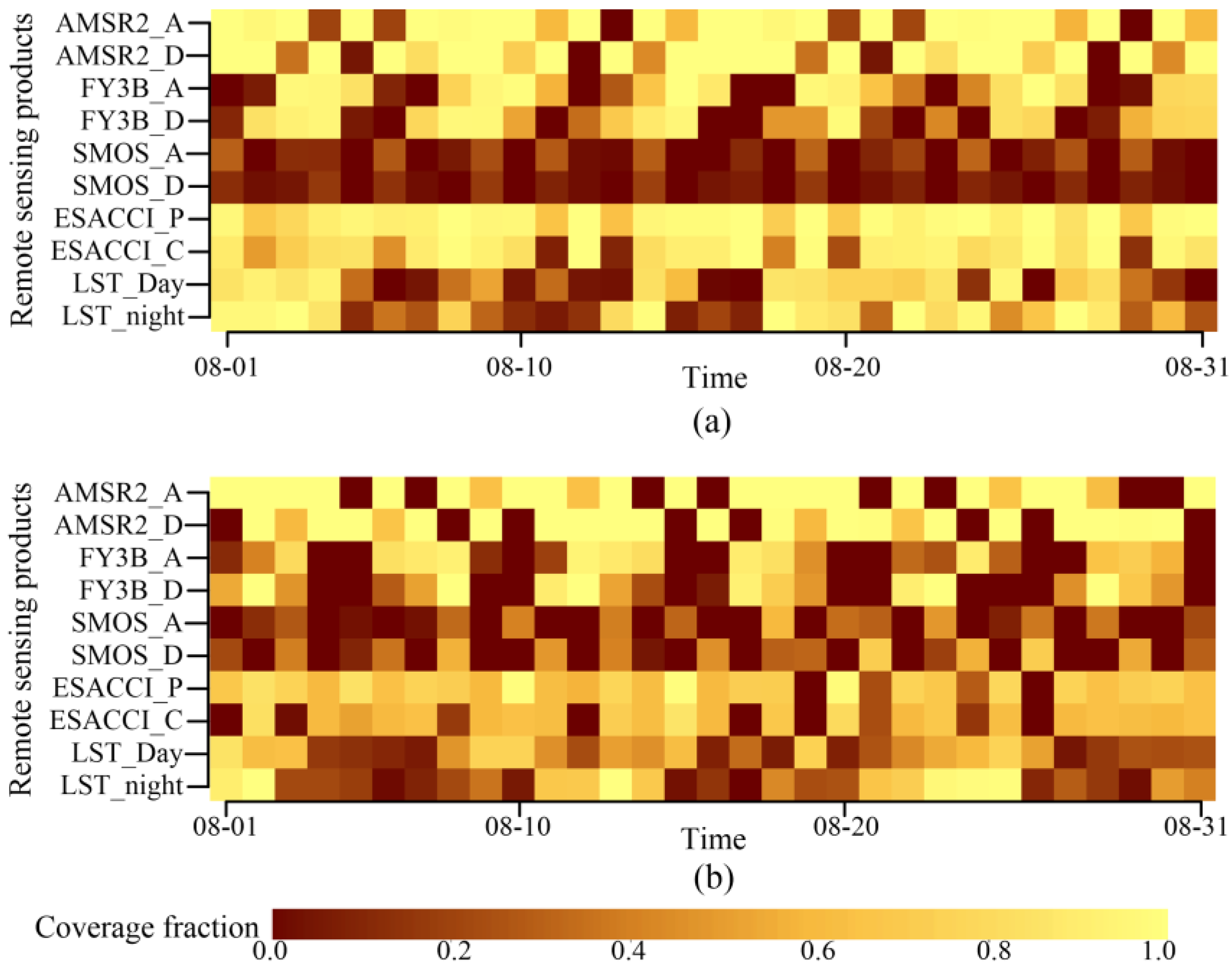
Figure 3 shows the daily coverage fractions of the remote sensing products for two experimental regions, including all the coarse SSM products and the LST products, during August 2012. Because of a lack of full-coverage daily data in the above coarse SSM products, as well as in the LST products listed below, only coincident dates with high fractions of data coverage (>0.5) were selected from the one-month study period. We used a kriging interpolation technique for the interpolation of uncovered pixels of SSM data in two experimental regions. To maintain consistency between the various coarse SSM products and the LST products, different dates within the period of interest were available. In the case of the upper HBR area, 13, 14, 10, 12, 10, and 12 days were selected for the AMSR2_A, AMSR2_D, FY3B_A, FY3B_D, ESACCI_C, and ESACCI_P products, respectively. For the Naqu area, 13, 10, 6, 4, 7, 8, 6, and 6 days were selected for the AMSR2_A, AMSR2_D, SMOS_A, SMOS_D, FY3B_A, FY3B_D, ESACCI_C, and ESACCI_P products, respectively.
3.2.4. MODIS Products
The LST, NDVI, and albedo were selected as auxiliary variables for the SSM downscaling. Three Moderate Resolution Imaging Spectroradiometer (MODIS) optical products at 1 km spatial resolution were used in conjunction with the Version 5 or 6 products of Aqua (downloaded from the website https://lpdaac.usgs.gov/). MODIS Aqua is a satellite in low earth orbit with equatorial crossing times of approximately 13:30 and 1:30 local solar time for the ascending and descending nodes, respectively. The day and night LSTs and NDVI data were extracted from the Version 6 daily LST product (MYD11A1) and 16-d NDVI product (MYD11A1), respectively. The BSA data were acquired from the Version 5 16-d albedo product (MCD43B3). The MCD43B3 provides the black-sky and white-sky albedo information based on shortwave radiation, and their linear combination could be taken to represent the BSA with weightings of 0.34 for the former and of 0.66 for the latter. The two 16 d products are cloud free; however, the daily LST products do not provide full-coverage data because of the influence of cloud. As mentioned in relation to the coarse SSM products, LST data on several coincident dates were selected for preparation for downscaling, and these were interpolated in cloud-covered regions using the kriging method. All MODIS products for the two experimental areas were projected and extracted consistently with the coarse SSM product, and their average aggregations were achieved at coarse grids of 25 km × 25 km.
3.3. Process of Experiment Implementation
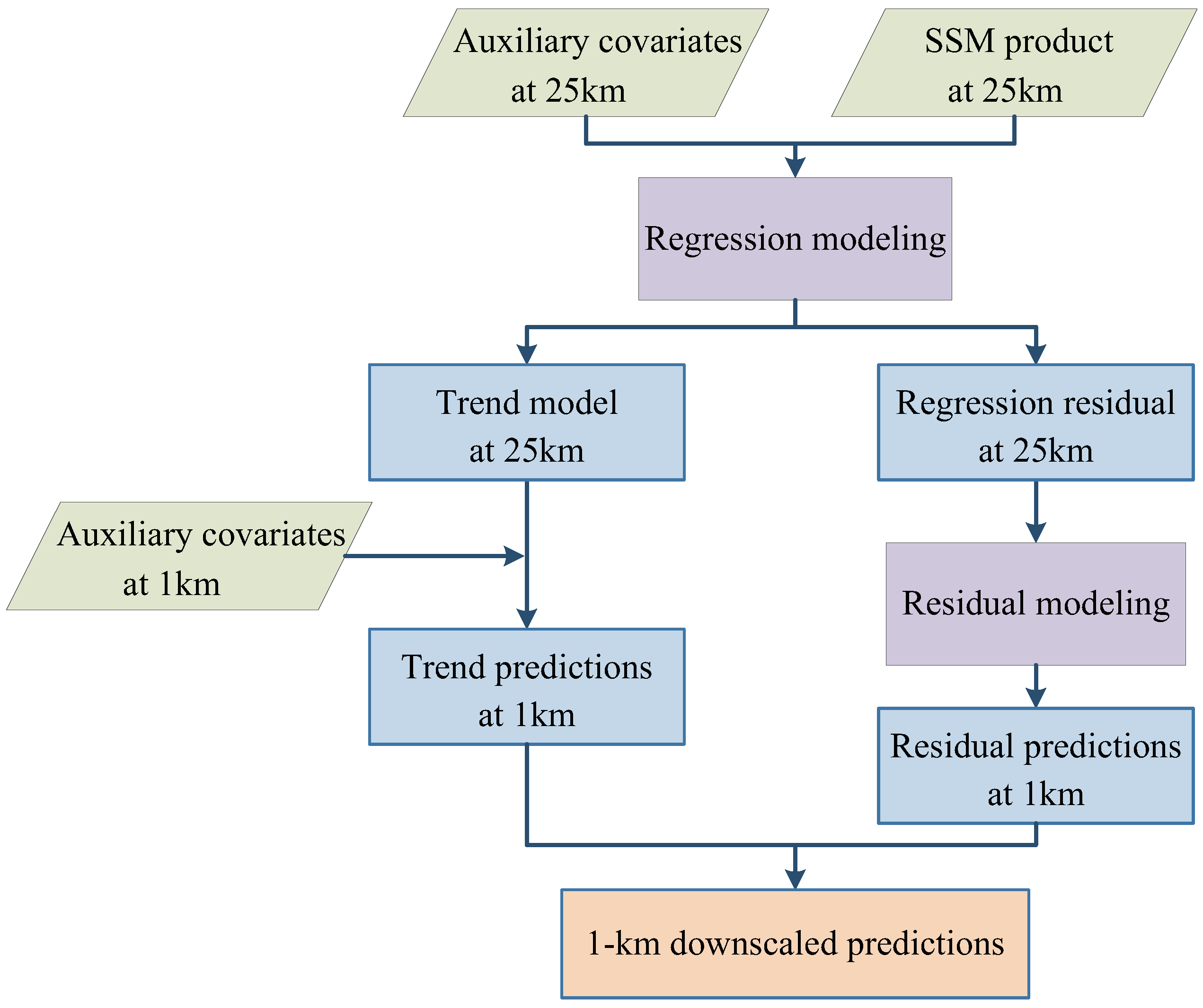
The two experimental regions in China, adopted to make the evaluation results more reliable, comprised the upper HRB area and the Naqu area, Tibet (Figure 1). Processing of all data is an essential step prior to the implementation of any downscaling method and validation. Under the same grid system, 25 km-resolution coarse SSM data and 25 km-resolution and 1 km-resolution related variables were preprocessed using resampling or average aggregation, as well as kriging interpolation, to fill gaps and compensate for non-full coverage. Figure 4 displays the simplified flowchart of downscaling method, which the downscaled perditions are consisted of trend and residual components. And Table 2 presents the details of the two study areas and the downscaling strategies adopted in this research.
There were eight groups of four coarse SSM products from the AMSR-2, ESA CCI, FY-3B, and SMOS, and six groups from the AMSR-2, ESA CCI, and FY-3B, for downscaling to 1 km resolution from 25 km resolution for Naqu and upper HBR areas, respectively. The downscaling methods were not applied on SMOS products in the upstream area of the HRB, because of the lack of data during August 2012. For convenience, we use a universal description, eight groups of four coarse SSM products in the subsequent analysis. The four downscaling methods that consisted of the trend model and the residual model were implemented on each coarse SSM product by incorporating three auxiliary variables (LST, NDVI, and BSA). The different trend models were established between SSM and its covariates at 25 km spatial resolution. Based on the scale-invariant assumption of the trend model, these regression models (i.e., GWR, quadratic regression, ordinary linear regression and SVR for the different downscaling methods) were used to predict the 1 km SSM spatial trend by incorporation of the fine covariates. Then, the different interpolation models were applied to downscale the 25 km residuals to 1 km resolution using the ATPK and bilinear methods. Considering that the trend model is always the core of the traditional statistical regression and machine learning methods [52,53,54], this experiment chose a simple common interpolation to deal with the residual components in QRM and SVR. Because of the limited referenced dataset, direct, indirect, and cross validation methods were adopted to analyze the downscaled predictions. In addition to the benefit from the high-quality SSM information of the ground-based measurements, an independent bias correction [55,56] was applied before implementation of the downscaling process for the case of the Naqu area, which comprised subtracting the bias (mean difference) between each coarse SSM product and the ground-based measurements from the coarse SSM products.
The brightness temperature (Tb) is a variable that strongly reflects the spatial variation of SSM. In the upstream area of the HBR, indirect comparisons between different 1 km SSM values predicted from various coarse SSM data using different downscaling methods and Tb values were performed, and the differences with in situ observations in the Naqu area were compared directly. To compare the influences of different coarse SSM products on the downscaled predictions of each method, cross validations were adopted in both areas in the absence of ground-based observations using triple collocation (TC) analysis [57,58]. The TC method can provide an estimation of error variances for three or more products of the same variable produced by mutually independent methods, and TC studies for SSM mainly use only three datasets [59]. There were different available days for various downscaled predictions, such as SMOS-based 1 km predictions for the upper HBR area were absent, and only limited predictions were available for a few available days for the Naqu area because of a lack of input information for the downscaling models. Hence, we applied TC analyses on the predictions based on each three coarse SSM products and calculated the mean of TC results. The methods and analyses adopted in this study were performed mainly using R software [60].
4. Results and Discussion
The experiments were run for eight groups of four 25 km SSM products for August 2012 in the upper HBR area and the Naqu area, where different dates for each case were selected according to the availability of input data. The downscaled 1 km predictions were tested using three validation methods. For direct validation, the downscaled predictions were compared with ground-based observations using several statistical parameters, including the root mean square error (RMSE) (m3·m−3), mean error (ME) (m3·m−3), correlation coefficient (R), and slope (SLOP) of linear regression between ground observations and downscaled predictions. The lower the ME, the lower the RMSE and higher the value of R that would be expected. The closer SLOP is to 1, the better the results would be. This direct validation was applied only in the Naqu area because of the lack of in situ measurements from the upper HBR area during the period of interest. Hence, indirect validation was used in the upper HBR area by adopting the H-Tb as a reference dataset. The R and the histogram-matching method [61], used for the comparisons between the 1 km H-Tb data and the 1 km downscaled predictions, involved calculating the intersection distance (ID) and Kullback–Leibler divergence (K–L). For the cross validation of the downscaled results in both experimental regions, TC analysis was repeated for each of the three datasets for the ascending cases (two cases for ESA CCI) and descending cases (two cases for ESA CCI).
4.1. Downscaled Results
Figure 5 displays the 1 km trend predictions of GWATPRK from different coarse SSM products acquired on August 14 for the upstream HBR area and on August 13 for the Naqu area. Only on these two days were all of the input remotely sensed data available, i.e., 24 and 32 downscaled images were obtained for the upper HBR and the Naqu areas, respectively. Figure 6 and Figure 7 display various coarse SSM products at 25 km resolution, together with corresponding downscaled images for the two experimental regions on these two days, respectively. It shows substantial discrepancies between 1 km trend predictions and corresponding 1 km downscaled predictions. Although the GWR model in GWATPRK method can capture the spatial local heterogeneity and the trend images also perform some spatial variations, it still lost some spatial information in trend predictions which could be compensated by using the residual interpolation. In downscaled images (Figure 6 and Figure 7), the white and green areas reflect the highest and lowest SSM values. For the upper HBR area, the areas with low elevation and several streams have the high SSM values. The top right corner in each image has the lowest elevation, but not always own high SSM values, which might be due to rare vegetation. For the Naqu area, the areas with low elevation have the high SSM values. There is almost no surface water in the Naqu area, and elevation shows considerable influence on SSM. Under a cold climate, elevation is one of the primary factors affecting the spatial distribution of SSM, and they show an inverse correlation. On both days, the downscaled images obtained using the GWATPRK and ATPRK methods show spatial patterns that have greater similarities with the coarse images than these of the QRM and SVR methods; this is because the latter two methods ignore spatial autocorrelation. The spatial patterns obtained using the SVR method are excessively fragmented for the same reason. Although the visual representation does not illustrate the achievement of any obvious improvements through use of the GWATPRK method, the following validations demonstrate its improved performance.
The cumulative distribution function (CDF) was employed to display the downscaled predictions by describing the percentage of occurrences of each value. As an example, Figure 8 shows the CDF curves of coarse SSM products and their corresponding downscaled predictions for the upper HBR. In each case (i.e., each image), one color is for one available day. The CDF curves of the downscaled images are similar to the coarse ones. To a certain extent, the differences between the curves of the four downscaling methods are less obvious visually than those of the spatial patterns. The QRM and SVR methods might not obtain poor values in terms of magnitude, but they are unsatisfactory in terms of their spatial distribution patterns.
The above-mentioned downscaling methods assumed the trend model between target variable and its auxiliary variables is scale-invariant. This scale-invariance has been applied in most of the downscaling methods which combines the auxiliary variables [62,63]. However, the established trend model at coarse spatial resolution might not simulate the relationships at fine spatial resolutions effectively. It might perform better in the case of a smaller scale factor than a larger scale factor. If there are multiscale information of target and auxiliary variables, it would be better to fuse these data in a downscaling process. The proposed downscaling method could be used repeatedly at different resolution for narrowing the scale factor.
The auxiliary variables would explain the spatial distribution of the unknown target variable at fine resolution. They are one of the key points for the type of downscaling methods which combines auxiliary variables. The satellite-based LST, NDVI, and BSA could represent the strong spatial variations, while the 16 day and 8 day composite product would be weak temporal variations. These temporal variations were ignored in the proposed GWATPRK, which is a spatial downscaling method. It might improve the accuracy of downscaled predictions by incorporating temporal variations, because the temporal detailed information would help capture the spatial–temporal variability of target variable. The time analysis is a little difficult during a short period (e.g., one-month), so the long time series analysis could be considerable in future research work. In addition, the problem of coincided time among each satellite-based SSM product and satellite-based auxiliary variable is really an unsolved issue in downscaling with remotely sensed products so far. For example, the coarse SSM products were obtained on daily observations, while the NDVI data were 16 day composites. The multisource data or temporal interpolation might be possible solutions.
4.2. Direct Validation
Direct validation was implemented in the Naqu area using the ground-based observations. Table 3 shows the spatial statistics of comparisons between each of the downscaled predictions from the eight groups of four coarse products and in situ measurements. The comparison results include the RMSE, ME, R, and SLOP. For the downscaled predictions of the four downscaling methods, smaller values of RMSE and ME were obtained when using the GWATRPK method compared with the other three methods. It illustrates the satisfactory performance of the proposed method in downscaling each coarse SSM product. The QRM method had the lowest RMSE and ME values, while the performances of the SVR and ATPRK methods were not distinguishable explicitly. This might be attributable to the use of ATPK in the ATPRK method and to the use of SVR in the SVR-based method.
For downscaled predictions based on the different coarse SSM products, the ESA CCI products (i.e., ESACCI_C and ESACCI_P) produced the most accurate results in comparison with the others. The 1 km predictions from the ascending products (i.e., AMSR2_A and FY3B_A) were better than from the descending products (i.e., AMSR2_D and FY3B_D) with lower RMSE and ME in the cases of both AMSR-2 and FY-3B. Conversely, the downscaled predictions from SMOS_D were closer to the ground-based observations because of the different times of equator crossing of AMSR-2 and FY-3B. This might be related to fewer errors in the AMSR2_A, SMOS_D, and FY3B_A products, which benefit from stable LSTs in the retrieval process of coarse SSM. However, as Table 3 shows, there are still rather substantial discrepancies between downscaled predictions and ground-based observations. This might be related not only to the prediction errors of the downscaling models and to the measurement errors of the original SSM observations and multiscale auxiliary variables, but also to the representativeness errors of the point support and 1 km × 1 km grid support. The trend models between SSM and its covariates were assumed to be scale-invariant at coarse and fine spatial resolution. Since there is always one ground station within a 1 km × 1 km grid, the spatial representativeness of ground observations were not matched well with the corresponding 1 km × 1 km grid. It is clear that with the smallest RMSE value of 0.056 m3·m−3, smallest ME absolute value of 0.002 m3·m−3, highest R value of 0.772 and better SLOP value of 1.036, the GWATPRK method using the ESACCI_C product resulted in the greatest accuracy. On average, when using the GWATPRK method, the RMSE values decreased by 26.4%, 13.2%, and 13.0% compared with the QRM, ATPRK, and SVR downscaling methods, respectively.
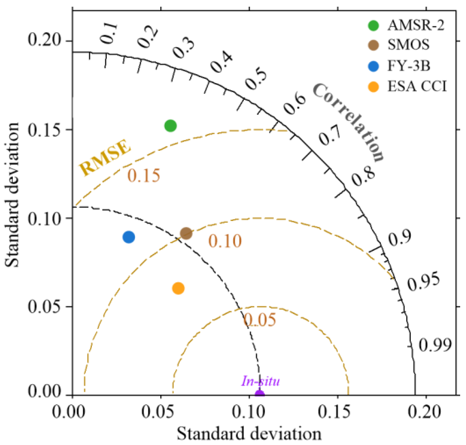
A simple Taylor diagram displaying statistical comparisons between 1 km SSM downscaled predictions combining two cases and ground-based measurements for AMSR-2, SMOS, FY-3B, and ESA CCI is shown in Figure 9. The comparisons are illustrated using three statistical parameters: standard deviation, R, and RMSE. The downscaled predictions from ESA CCI have the highest R and lowest RMSE among the downscaled remotely sensed products. The SMOS products produced better predictions than AMSR-2, with comparatively lower RMSE and higher R values. SMOS is designed specifically for SSM observation, and it exploits the L band, which is better than either the C band or the X band for SSM retrieval. Lower values of RMSE indicate greater accuracy of the downscaled predictions. The small errors of the coarse SSM products and input auxiliary variables lead to lower RMSE and higher R values. The MYD11A1 LST product used with both SMOS and ESA CCI did not match well with their equator crossing times. Therefore, the MODIS MOD11A1 for SMOS and average LST for ESA CCI could be adopted in the future.
4.3. Indirect Validation
Indirect validation was implemented in the upper HBR area because of the lack of ground-based observations. Comparisons on 1 August 2012, between the downscaled predictions and the H-Tb data illustrated in Table 4, are based on calculating the similarity between images using three metrics: R, ID, and K–L. The SSM data and H-Tb data were normalized by maximum and minimum. Higher R and closer distances (i.e., a large ID value and small K–L value) mean the downscaled predictions are more accurate. The comparison results were found consistent with the direct validation results across the different cases.
For the four downscaling methods, GWATPRK produced the highest accuracy of the downscaled predictions, while ESA CCI had the closet distance for the various coarse SSM products. The ESACCI_C with GWATPRK produced the best performance with the largest values of R (0.703) and ID (0.589), and the smallest K–L value of 0.542. The SVR performed better than ATPRK in distance metrics, and it also outperformed GWATPRK with AMSR2_A, where the differences between SVR and ATPRK in direct validation were not obvious. Some advantages of the spatial statistical methods might be hidden when using histogram-matching methods. The image histogram expresses the probability distribution of the values, while histogram matching does not consider pixel positions. Moreover, the values of K–L were all >0.5. On the one hand, the remotely sensed coarse SSM products for the upper HBR area have not undergone bias correction; thus, any underestimations or overestimations in the original data would affect prediction accuracy. On the other hand, the H-Tb representativeness of SSM is limited; therefore, retrievals of SSM based on Tb data could be employed as a reference dataset to enforce direct validation. However, a retrieval model would also introduce some error and enhance error propagation, which would need to be taken into account.
4.4. Cross Validation
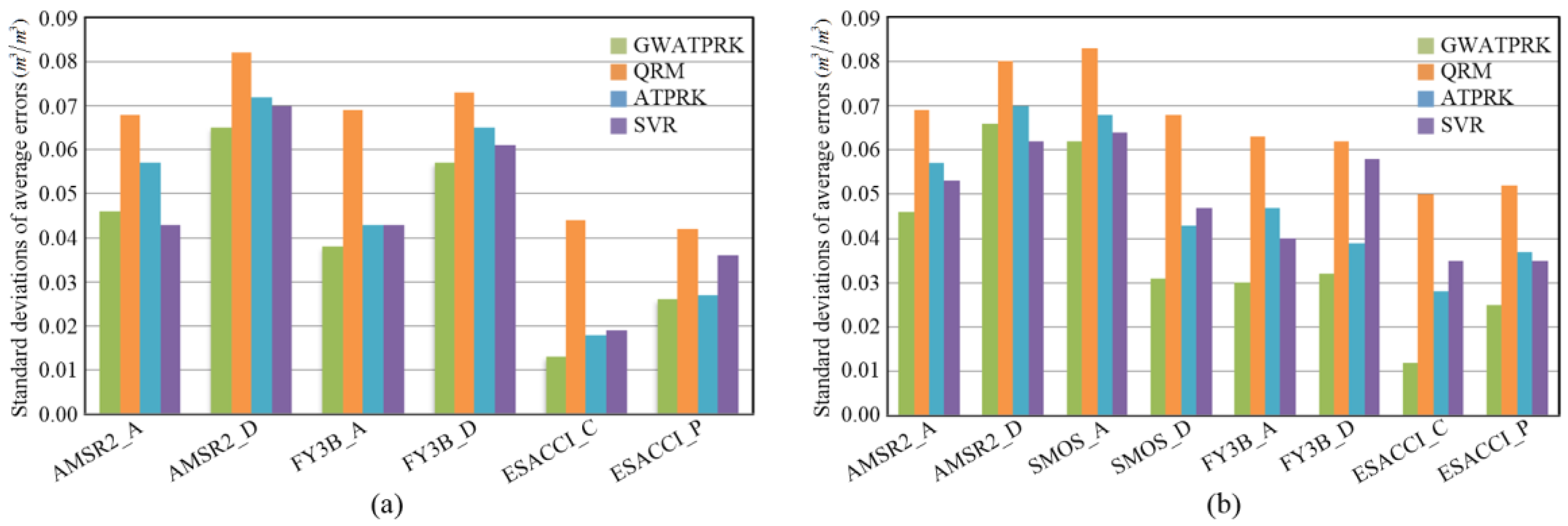
Cross validation among the various downscaled predictions was implemented using TC analysis for the upstream HBR and Naqu areas. The standard deviations of the average errors of the 1 km predictions for each coarse SSM product for both experimental areas are shown in Figure 10. The advantage of the use of the GWATPRK method in spatial downscaling is obvious compared with the three other methods. The downscaled predictions using the mean of results of four methods, arranged in ascending order of error values, are ESACCI_C (0.024 m3·m−3) < ESACCI_P (0.033 m3·m−3) < FY3B_A (0.048 m3·m−3) < AMSR2_A (0.054 m3·m−3) < FY3B_D (0.064 m3·m−3) < AMSR2_D (0.072 m3·m−3) for the upper HBR area, and are ESACCI_C (0.031 m3·m−3) < ESACCI_P (0.037 m3·m−3) < FY3B_A (0.045 m3·m−3) < SMOS_D (0.047 m3·m−3) < FY3B_D (0.048 m3·m−3) < AMSR2_A (0.056 m3·m−3) < SMOS_A (0.069 m3·m−3) < AMSR2_D (0.070 m3·m−3) for the Naqu area. The EASCCI_C produced downscaled predictions with the best accuracy of the various coarse SSM products. This might be attributable to the better quality of the EASCCI_C product, which combines different active and passive SM products.
In this paper, only three auxiliary variables (LST, NDVI, and BSA) were considered in this study, which might have limited the scope of the proposed method. When the further multiple covariates carry complementary information about SSM, the selection of such covariates is encouraged to improve the performance of downscaling. Additional auxiliary covariates, such as soil temperature, evapotranspiration, and apparent thermal inertia could be incorporated easily. The categorical variables, such as soil type and land cover, could be included in the downscaling process via stratification. The relief-derived wetness indices could also be employed as covariates. In the ATP downscaling method, the target fine grids of the remote sensing images refer to points, where the central point value is used to represent the grid value. Sometimes, this might not work particularly well, especially for fine grids with strong heterogeneity. Thus, downscaling accuracy could be enhanced by adopting average or weighted average values at finer resolution, if finer information exists, to capture the spatial variation of the target variable. In addition, the bilinear interpolation was applied to deal with the coarse regression residuals of QRM and SVR methods. This common simple spatial interpolation technique did not consider the change of support during downscaling process, which might cause more prediction errors. When their coarse residuals have the spatial autocorrelation and satisfy the requirement of stationarity, it is an interesting point of research to incorporate the QRM and SVR with ATPK. Furthermore, the accuracy of downscaling predictions could be questionable given the complex interactions among the errors of the input variables and the downscaling model. In future research, error analyses should be explored.
5. Conclusions
Spatial downscaling is often applied to transform coarse-resolution remotely sensed products to fine resolution for monitoring subtle surface features. This paper described the development of a new spatial downscaling approach that integrates GWR and ATPK. The GWATPRK has the dual advantages of addressing local spatial heterogeneity and spatial correlation between target variable and covariates. To demonstrate the efficacy of this method, it was applied to various coarse SSM products in the upstream of the HRB area and in the Naqu area during a one month period. Comparisons of the different downscaled predictions obtained from GWATPRK and three other benchmark methods showed that GWATPRK performed better, not only in direct validation, but also in indirect and cross validations. Cross validation indicated that the downscaled predictions from ESA CCI products were the most accurate, where the use of coarse input data with fewer errors increased the downscaling accuracy. As a general method, the proposed downscaling method could also be extended for almost all continuous variables in other study areas. Besides the point ground SSM measurements, other ground-based observations such as cosmic-ray neutron measurements [64,65] could also serve for validation purpose. In addition, these ground measurements might be considered as auxiliary variables in downscaling process, which would enhance the accuracy of downscaled predictions benefitting from the high-quality data. However, the limitations regarding input data coverage and spatiotemporal downscaling should be explored in future research.
Acknowledgments
This work was jointly supported by the National Natural Science Foundation for Distinguished Young Scholars of China under Grant 41725006, two Key Programs of the National Natural Science Foundation of China under Grant 41531174 and Grant 41531179 and the Science Fund for Creative Research Groups of the National Natural Science Foundation of China under Grant 41421001. We thank Jian Kang for providing suggestions regarding the validations and we are grateful to all the data providers. We thank James Buxton MSc from Liwen Bianji, Edanz Group China (www.liwenbianji.cn./ac), for editing the English text of this manuscript.
Author Contributions
Yong Ge and Jianghao Wang developed the concept and conceived the research plan; Gerard B.M. Heuvelink further improved the method and the experiments; Yan Jin performed the experiments and analyzed the data; Le Wang provided many helpful suggestions and modified this manuscript. All authors shared equally in the editing of the manuscript.
Conflicts of Interest
The authors declare no conflict of interest.
References
- Hall, F.G.; Townshend, J.R.; Engman, E.T. Status of remote sensing algorithms for estimation of land surface state parameters. Remote Sens. Environ. 1995, 51, 138–156. [Google Scholar] [CrossRef]
- Zavorotny, V.U.; Voronovich, A.G. Scattering of GPS signals from the ocean with wind remote sensing application. IEEE Trans. Geosci. Remote Sens. 2002, 38, 951–964. [Google Scholar] [CrossRef]
- Kaufman, Y.J.; Tanré, D.; Remer, L.A.; Vermote, E.F.; Chu, A.; Holben, B.N. Operational remote sensing of tropospheric aerosol over land from EOS moderate resolution imaging spectroradiometer. J. Geophys. Res. 1997, 102, 17051–17067. [Google Scholar] [CrossRef]
- Atkinson, P.M.; Tate, N.J. Spatial scale problems and geostatistical solutions: A review. Prof. Geogr. 2000, 52, 607–623. [Google Scholar] [CrossRef]
- Peng, J.; Loew, A.; Merlin, O.; Verhoest, N.E.C. A review of spatial downscaling of satellite remotely-sensed soil moisture. Rev. Geophys. 2017, 55, 341–366. [Google Scholar] [CrossRef]
- Atkinson, P.M. Downscaling in remote sensing. Int. J. Appl. Earth Obs. Geoinf. 2012, 22, 106–114. [Google Scholar] [CrossRef]
- Chen, Y.H.; Ge, Y.; Jia, Y.X. Integrating object boundary in super-resolution land-cover mapping. IEEE J. Sel. Top. Appl. Earth Obs. Remote Sens. 2017, 10, 219–230. [Google Scholar] [CrossRef]
- Bergant, K.; Kajfež-Bogataj, L.; Črepinšek, Z. Statistical downscaling of general-circulation-model- simulated average monthly air temperature to the beginning of flowering of the dandelion (Taraxacum officinale) in Slovenia. Int. J. Biometeorol. 2002, 46, 22–32. [Google Scholar] [CrossRef] [PubMed]
- Pardo-Igúzquiza, E.; Chica-Olmo, M.; Atkinson, P.M. Downscaling cokriging for image sharpening. Remote Sens. Environ. 2006, 102, 86–98. [Google Scholar] [CrossRef]
- Hutengs, C.; Vohland, M. Downscaling land surface temperatures at regional scales with random forest regression. Remote Sens. Environ. 2016, 178, 127–141. [Google Scholar] [CrossRef]
- Wood, A.W.; Leung, L.R.; Sridhar, V.; Lettenmaier, D.P. Hydrologic implications of dynamical and statistical approaches to downscaling climate model outputs. Clim. Chang. 2004, 62, 189–216. [Google Scholar] [CrossRef]
- Rahman, S.; Bagtzoglou, A.C.; Hossain, F.; Tang, L.; Yarbrough, L.; Easson, G. Investigating spatial downscaling of satellite rainfall data for streamflow simulation in a medium-sized basin. J. Hydrometeorol. 2008, 10, 1063–1079. [Google Scholar] [CrossRef]
- Tao, K.; Barros, A.P. Using fractal downscaling of satellite precipitation products for hydrometeorological applications. J. Atmos. Ocean. Technol. 2010, 27, 409–427. [Google Scholar] [CrossRef]
- Kaheil, Y.H.; Rosero, E.; Gill, M.K.; Mckee, M.; Bastidas, L.A. Downscaling and forecasting of evapotranspiration using a synthetic model of wavelets and support vector machines. IEEE Trans. Geosci. Remote Sens. 2008, 46, 2692–2707. [Google Scholar] [CrossRef]
- Cressie, N.A. Change of support and the modifiable unit problem. Geogr. Syst. 1996, 3, 159–180. [Google Scholar]
- Gotway, C.A.; Young, L.J. Combining incompatible spatial data. J. Am. Stat. Assoc. 2002, 97, 632–648. [Google Scholar] [CrossRef]
- Kyriakidis, P.C. A geostatistical framework for area-to-point spatial interpolation. Geogr. Anal. 2004, 36, 259–289. [Google Scholar] [CrossRef]
- Yoo, E.H.; Kyriakidis, P.C. Area-to-point kriging with inequality-type data. J. Geogr. Syst. 2006, 8, 357–390. [Google Scholar] [CrossRef]
- Goovaerts, P. Geostatistical analysis of disease data: Accounting for spatial support and population density in the isopleth mapping of cancer mortality risk using area-to-point poisson kriging. Int. J. Health Geogr. 2006, 5, 52. [Google Scholar] [CrossRef] [PubMed]
- Yoo, E.H.; Kyriakidis, P.C.; Tobler, W. Reconstructing population density surfaces from areal data: A comparison of Tobler’s pycnophylactic interpolation method and area-to-point kriging. Geogr. Anal. 2010, 42, 78–98. [Google Scholar] [CrossRef]
- Yoo, E.H.; Kyriakidis, P.C. Area-to-point kriging in spatial hedonic pricing models. J. Geogr. Syst. 2009, 11, 381–406. [Google Scholar] [CrossRef]
- Kerry, R.; Goovaerts, P.; Haining, R.P.; Ceccato, V. Applying geostatistical analysis to crime data: Car-related thefts in the Baltic States. Geogr. Anal. 2010, 42, 53–77. [Google Scholar] [CrossRef] [PubMed]
- Atkinson, P.M.; Pardo-Iguzquiza, E.; Chica-Olmo, M. Downscaling cokriging for super-resolution mapping of continua in remotely sensed images. IEEE Trans. Geosci. Remote Sens. 2008, 46, 573–580. [Google Scholar] [CrossRef]
- Wang, Q.M.; Shi, W.Z.; Atkinson, P.M. Area-to-point regression kriging for pan-sharpening. ISPRS J. Photogramm. Remote Sens. 2016, 114, 151–165. [Google Scholar] [CrossRef]
- Kerry, R.; Goovaerts, P.; Rawlins, B.G.; Marchant, B.P. Disaggregation of legacy soil data using area to point kriging for mapping soil organic carbon at the regional scale. Geoderma 2012, 170, 347–358. [Google Scholar] [CrossRef] [PubMed] [Green Version]
- Wang, Q.M.; Shi, W.Z.; Atkinson, P.M.; Zhao, Y. Downscaling MODIS images with area-to-point regression kriging. Remote Sens. Environ. 2015, 166, 191–204. [Google Scholar] [CrossRef]
- Hengl, T.; Heuvelink, G.B.M.; Rossiter, D.G. About regression-kriging: From equations to case studies. Comput. Geosci. 2007, 33, 1301–1315. [Google Scholar] [CrossRef]
- Liu, X.H.; Kyriakidis, P.C.; Goodchild, M.F. Population-density estimation using regression and area-to-point residual kriging. Int. J. Geogr. Inf. Sci. 2008, 22, 431–447. [Google Scholar] [CrossRef]
- Poggio, L.; Gimona, A. Modelling high resolution RS data with the aid of coarse resolution data and ancillary data. Int. J. Appl. Earth Obs. Geoinf. 2013, 23, 360–371. [Google Scholar] [CrossRef]
- Zhang, Y.H.; Atkinson, P.M.; Ling, F.; Wang, Q.M.; Li, X.D.; Shi, L.F.; Du, Y. Spectral–spatial adaptive area-to-point regression kriging for MODIS image downscaling. IEEE J. Sel. Top. Appl. Earth Obs. Remote Sens. 2017, 10, 1883–1896. [Google Scholar] [CrossRef]
- Wang, Q.M.; Shi, W.Z.; Atkinson, P.M.; Wei, Q. Approximate area-to-point regression kriging for fast hyperspectral image sharpening. IEEE J. Sel. Top. Appl. Earth Obs. Remote Sens. 2017, 10, 286–295. [Google Scholar] [CrossRef]
- Goodchild, M.F. The Validity and Usefulness of Laws in Geographic Information Science and Geography. Ann. Assoc. Am. Geogr. 2004, 94, 300–303. [Google Scholar] [CrossRef]
- Fotheringham, A.S.; Charlton, M.E.; Brunsdon, C. Geographically weighted regression: A natural evolution of the expansion method for spatial data analysis. Environ. Plan. A Econ. Space 1998, 30, 1905–1927. [Google Scholar] [CrossRef]
- Harris, P.; Fotheringham, A.S.; Crespo, R.; Charlton, M. The use of geographically weighted regression for spatial prediction: An evaluation of models using simulated data sets. Math. Geosci. 2010, 42, 657–680. [Google Scholar] [CrossRef]
- Zhao, N.; Chen, C.F.; Zhou, X.; Yue, T.X. A comparison of two downscaling methods for precipitation in china. Environ. Earth Sci. 2015, 74, 6563–6569. [Google Scholar] [CrossRef]
- Kumari, M.; Singh, C.K.; Bakimchandra, O.; Basistha, A. Geographically weighted regression based quantification of rainfall–topography relationship and rainfall gradient in central himalayas. Int. J. Climatol. 2017, 37, 1299–1309. [Google Scholar] [CrossRef]
- Jin, Y.; Ge, Y.; Wang, J.H.; Chen, Y.H.; Heuvelink, G.B.M.; Atkinson, P.M. Downscaling amsr-2 soil moisture data with geographically weighted area-to-area regression kriging. IEEE Trans. Geosci. Remote Sens. 2017, 56, 1–15. [Google Scholar] [CrossRef]
- Jin, Y.; Ge, Y.; Wang, J.H.; Heuvelink, G.B.M. Deriving temporally continuous soil moisture estimations at fine resolution by downscaling remotely sensed product. Int. J. Appl. Earth Obs. Geoinf. 2018, 68, 8–19. [Google Scholar] [CrossRef]
- Piles, M.; Camps, A.; Vall-Llossera, M.; Corbella, I.; Panciera, R.; Rudiger, C.; Kerr, Y.; Walker, J. Downscaling SMOS-derived soil moisture using MODIS visible/infrared data. IEEE Trans. Geosci. Remote Sens. 2011, 49, 3156–3166. [Google Scholar] [CrossRef]
- Tripathi, S.; Srinivas, V.V.; Nanjundiah, R.S. Downscaling of precipitation for climate change scenarios: A support vector machine approach. J. Hydrol. 2006, 330, 621–640. [Google Scholar] [CrossRef]
- Hengl, T.; Heuvelink, G.B.M.; Stein, A. A generic framework for spatial prediction of soil variables based on regression-kriging. Geoderma 2004, 120, 75–93. [Google Scholar] [CrossRef]
- Goovaerts, P. Kriging and semivariogram deconvolution in the presence of irregular geographical units. Math. Geosci. 2008, 40, 101–128. [Google Scholar] [CrossRef]
- Zawadzki, J.; Cieszewski, C.J.; Zasada, M.; Lowe, R.C. Applying geostatistics for investigations of forest ecosystems using remote sensing imagery. Silva Fenn. 2005, 39, 599–617. [Google Scholar] [CrossRef]
- Li, X.; Cheng, G.D.; Liu, S.M.; Xiao, Q.; Ma, M.G.; Jin, R.; Che, T.; Liu, Q.H.; Wang, W.Z.; Qi, Y.; et al. Heihe Watershed Allied Telemetry Experimental Research (HiWATER): Scientific objectives and experimental design. Bull. Am. Meteorol. Soc. 2013, 94, 1145–1160. [Google Scholar] [CrossRef]
- Yang, K.; Qin, J.; Zhao, L.; Chen, Y.Y.; Tang, W.J.; Han, M.L.; La, Z.; Chen, Z.Q.; Lv, N.; Ding, B.H.; et al. A multi-scale soil moisture and freeze-thaw monitoring network on the third pole. Bull. Am. Meteorol. Soc. 2013, 94, 1907–1916. [Google Scholar] [CrossRef]
- Zeng, J.Y.; Li, Z.; Chen, Q.; Bi, H.Y.; Qiu, J.X.; Zou, P.F. Evaluation of remotely sensed and reanalysis soil moisture products over the tibetan plateau using in-situ observations. Remote Sens. Environ. 2015, 163, 91–110. [Google Scholar] [CrossRef]
- Kim, S.; Balakrishnan, K.; Liu, Y.; Johnson, F.; Sharma, A. Spatial disaggregation of coarse soil moisture data by using high-resolution remotely sensed vegetation products. IEEE Geosci. Remote Sens. Lett. 2017, 14, 1604–1608. [Google Scholar] [CrossRef]
- Cui, C.; Xu, J.; Zeng, J.; Chen, K.S.; Bai, X.; Lu, H.; Chen, Q.; Zhao, T.J. Soil moisture mapping from satellites: An intercomparison of SMAP, SMOS, FY3B, AMSR2, and ESA CCI over two dense network regions at different spatial scales. Remote Sens. 2018, 10, 33. [Google Scholar] [CrossRef]
- Kerr, Y.H.; Waldteufel, P.; Wigneron, J.P.; Martinuzzi, J.M.; Font, J.; Berger, M. Soil moisture retrieval from space: The soil moisture ocean salinity (SMOS) mission. IEEE Trans. Geosci. Remote Sens. 2001, 39, 1729–1735. [Google Scholar] [CrossRef]
- Parinussa, R.M.; Wang, G.; Holmes, T.R.H.; Liu, Y.Y.; Dolman, A.J.; Jeu, R.A.M.D.; Jiang, T.; Zhang, P.; Shi, J. Global surface soil moisture from the microwave radiation imager onboard the Fengyun-3B satellite. Int. J. Remote Sens. 2014, 35, 7007–7029. [Google Scholar] [CrossRef]
- Dorigo, W.; Wagner, W.; Albergel, C.; Albrecht, F.; Balsamo, G.; Brocca, L. ESA CCI soil moisture for improved earth system understanding: State-of-the art and future directions. Remote Sens. Environ. 2017, 203, 185–215. [Google Scholar] [CrossRef]
- Sachindra, D.A.; Huang, F.; Barton, A.; Perera, B.J.C. Least square support vector and multi-linear regression for statistically downscaling general circulation model outputs to catchment streamflows. Int. J. Climatol. 2013, 33, 1087–1106. [Google Scholar] [CrossRef]
- Zhang, H.; Huang, B. Support vector regression-based downscaling for intercalibration of multiresolution satellite images. IEEE Trans. Geosci. Remote Sens. 2013, 51, 1114–1123. [Google Scholar] [CrossRef]
- Alaya, M.A.B.; Chebana, F.; Ouarda, T.B.M.J. Multisite and multivariable statistical downscaling using a gaussian copula quantile regression model. Clim. Dyn. 2016, 1–15. [Google Scholar] [CrossRef]
- Merlin, O.; Rudiger, C.; Bitar, A.A.; Richaume, P.; Walker, J.P.; Kerr, Y.H. Disaggregation of SMOS soil moisture in southeastern Australia. IEEE Trans. Geosci. Remote Sens. 2012, 50, 1556–1571. [Google Scholar] [CrossRef] [Green Version]
- Djamai, N.; Magagi, R.; Goïta, K.; Merlin, O.; Kerr, Y.; Roy, A. A combination of dispatch downscaling algorithm with class land surface scheme for soil moisture estimation at fine scale during cloudy days. Remote Sens. Environ. 2016, 184, 1–14. [Google Scholar] [CrossRef]
- Miralles, D.G.; Crow, W.T.; Cosh, M.H. Estimating spatial sampling errors in coarse-scale soil moisture estimates derived from point-scale observations. J. Hydrometeorol. 2010, 11, 1423–1429. [Google Scholar] [CrossRef]
- Kang, J.; Jin, R.; Li, X.; Zhang, Y.; Zhu, Z. Spatial Upscaling of Sparse Soil Moisture Observations Based on Ridge Regression. Remote Sens. 2018, 10, 192. [Google Scholar] [CrossRef]
- Yilmaz, M.T.; Crow, W.T. Evaluation of assumptions in soil moisture triple collocation analysis. J. Hydrometeorol. 2013, 15, 1293–1302. [Google Scholar] [CrossRef]
- R Core Team. R: A Language and Environment for Statistical Computing; R Foundation for Statistical Computing: Vienna, Austria, 2014; Available online: http://www.r-project.org/ (accessed on 27 March 2018).
- Cha, S.H.; Srihari, S.N. On measuring the distance between histograms. Pattern Recognit. 2002, 35, 1355–1370. [Google Scholar] [CrossRef]
- Bisquert, M.; Sánchez, J.M.; Caselles, V. Evaluation of disaggregation methods for downscaling modis land surface temperature to Landsat spatial resolution in Barrax test site. IEEE J. Sel. Top. Appl. Earth Obs. Remote Sens. 2016, 9, 1430–1438. [Google Scholar] [CrossRef]
- Eweys, O.A.; Escorihuela, M.J.; Villar, J.M.; Er-Raki, S.; Amazirh, A.; Olivera, L.; Jarlan, L.; Khabba, S.; Merlin, O. Disaggregation of SMOS soil moisture to 100 m resolution using MODIS optical/thermal and sentinel-1 radar data: Evaluation over a bare soil site in morocco. Remote Sens. 2017, 9, 1155. [Google Scholar] [CrossRef]
- Zreda, M.; Desilets, D.; Ferré, T.P.A.; Scott, R.L. Measuring soil moisture content non-invasively at intermediate spatial scale using cosmic-ay neutrons. Geophys. Res. Lett. 2008, 35, L21402. [Google Scholar] [CrossRef]
- Kędzior, M.A.; Zawadzki, J. SMOS data as a source of the agricultural drought information: Case study of the Vistula catchment, Poland. Geoderma 2017, 306, 167–182. [Google Scholar] [CrossRef]
Figure 1.
Locations and elevations of the two experimental regions: the upper HBR area and the Naqu area. The spatial distribution of the ground stations in the Naqu area and the arrangements of the coarse grid pixels for both areas are also shown.
Figure 1.
Locations and elevations of the two experimental regions: the upper HBR area and the Naqu area. The spatial distribution of the ground stations in the Naqu area and the arrangements of the coarse grid pixels for both areas are also shown.

Figure 2.
Daily SSM values for each coarse surface soil moisture (SSM) product during August 2012 in Naqu area. Dots denote the average value and the bars denote ±1 standard deviation.
Figure 2.
Daily SSM values for each coarse surface soil moisture (SSM) product during August 2012 in Naqu area. Dots denote the average value and the bars denote ±1 standard deviation.

Figure 3.
Daily coverage fractions of remote sensing products (i.e., eight groups of four coarse SSM products and MODIS LST) during August 2012 in two experimental regions: (a) upper HBR area and (b) Naqu area.
Figure 3.
Daily coverage fractions of remote sensing products (i.e., eight groups of four coarse SSM products and MODIS LST) during August 2012 in two experimental regions: (a) upper HBR area and (b) Naqu area.

Figure 4.
The simplified flowchart of downscaling method.

Figure 5.
One kilometer trend predictions of GWATPRK from different coarse SSM products in two experimental regions. (a) Upper HBR area on August 14 2012, and (b) Naqu area on 13 August 2012.
Figure 5.
One kilometer trend predictions of GWATPRK from different coarse SSM products in two experimental regions. (a) Upper HBR area on August 14 2012, and (b) Naqu area on 13 August 2012.

Figure 6.
Upper HBR area on 14 August 2012. (a) Various 25 km SSM images and downscaled 1 km SSM images derived using the four methods: (b) GWATPRK, (c) QRM, (d) ATPRK, and (e) SVR.
Figure 6.
Upper HBR area on 14 August 2012. (a) Various 25 km SSM images and downscaled 1 km SSM images derived using the four methods: (b) GWATPRK, (c) QRM, (d) ATPRK, and (e) SVR.

Figure 7.
Naqu area on 13 August 2012. (a) Various 25 km SSM images and downscaled 1 km SSM images derived using the four methods: (b) GWATPRK, (c) QRM, (d) ATPRK, and (e) SVR.
Figure 7.
Naqu area on 13 August 2012. (a) Various 25 km SSM images and downscaled 1 km SSM images derived using the four methods: (b) GWATPRK, (c) QRM, (d) ATPRK, and (e) SVR.

Figure 8.
CDF curves for various remotely sensed products on available days within one month in the upstream HBR area: (a) coarse 25 km SSM products and downscaled 1 km SSM predictions derived using the four methods: (b) GWATPRK, (c) QRM, (d) ATPRK, and (e) SVR.
Figure 8.
CDF curves for various remotely sensed products on available days within one month in the upstream HBR area: (a) coarse 25 km SSM products and downscaled 1 km SSM predictions derived using the four methods: (b) GWATPRK, (c) QRM, (d) ATPRK, and (e) SVR.

Figure 9.
Simple Taylor diagram displaying statistical comparisons between 1 km SSM downscaled predictions combining two cases and ground-based measurements for AMSR-2, SMOS, FY-3B, and ESA CCI. The in situ point is for all the validation data.
Figure 9.
Simple Taylor diagram displaying statistical comparisons between 1 km SSM downscaled predictions combining two cases and ground-based measurements for AMSR-2, SMOS, FY-3B, and ESA CCI. The in situ point is for all the validation data.

Figure 10.
Standard deviations of average errors of 1 km predictions from different coarse SSM products in two experimental regions: (a) upper HBR area and (b) Naqu area.
Figure 10.
Standard deviations of average errors of 1 km predictions from different coarse SSM products in two experimental regions: (a) upper HBR area and (b) Naqu area.


Table 1.
Summary of the satellite based SSM data.
| Data Source | Short Name | Spatial Resolution | Temporal Resolution | Coverage | |
|---|---|---|---|---|---|
| AMSR-2 | Ascending product | AMSR2_A | 25 km | Daily | Global 2012– |
| Descending product | AMSR2_D | ||||
| SMOS | Ascending product | SMOS_A | 25 km | Daily | Global 2010– |
| Descending product | SMOS_D | ||||
| FY-3B | Ascending product | FY3B_A | 25 km | Daily | Global 2011– |
| Descending product | FY3B_D | ||||
| ESA CCI | Combined product | ESACCI_C | 25 km | Daily | Global 1978–2016 |
| Passive product | ESACCI_P | ||||
Table 2.
Details of the two study areas and downscaling strategies used in this research.
| Study Area | Coarse SSM | Other Variables | Downscaling Method | Validation | ||
|---|---|---|---|---|---|---|
| Name | Trend | Residual | ||||
| Upper HRB area | AMSR-2 (25 km) ESA CCI (25 km) FY-3B (25 km) | LST (1 km/25 km) NDVI (1 km/25 km) BSA (1 km/25 km) Tb (1 km) | GWATPRK | GWR | ATPK | Cross validation using the TC method Indirect validation using Tb data |
| QRM | Quadratic regression | Bilinear interpolation | ||||
| ATPRK | Ordinary linear regression | ATPK | ||||
| SVR | Support vector regression | Bilinear interpolation | ||||
| Naqu area | AMSR-2 (25 km) ESA CCI (25 km) FY-3B (25 km) SMOS (25 km) | LST (1 km/25 km) NDVI (1 km/25 km) BSA (1 km/25 km) In situ (1 km) | GWATPRK | GWR | ATPK | Direct validation using ground observations Cross validation using the TC method |
| QRM | Quadratic regression | Bilinear interpolation | ||||
| ATPRK | Ordinary linear regression | ATPK | ||||
| SVR | Support vector regression | Bilinear interpolation | ||||
Notes. Tb stands for brightness temperature, which was only available on 1 August 2012 in the upstream area of the HRB, where ground observations are absent. These two other variables of Tb data and in situ observations were employed for validation and the other three variables (i.e., LST, NDVI, and BAS) were used as auxiliary variables for downscaling. Because of the lack of information in the case of SMOS, it was not possible to downscale SMOS in the upstream area of the HRB. The indirect and cross validations were used in the upper HRB area and the direct and cross validations were applied in the Naqu area.
Table 3.
Spatial statistics of comparisons between 1 km downscaled predictions and ground-based measurements for the different cases in the Naqu area. (The bold values represent the best performance of all downscaling predictions for each validation index. In each validation index, the values with * mean the best performance of different downscaling predictions from the same satellite-based SSM product.)
| AMSR2_A | AMSR2_D | SMOS_A | SMOS_D | FY3B_A | FY3B_D | ESACCI_C | ESACCI_P | ||
|---|---|---|---|---|---|---|---|---|---|
| RMSE | GWATPRK | 0.114 * | 0.175 * | 0.114 * | 0.083 * | 0.079 * | 0.195 * | 0.056 * | 0.075 * |
| QRM | 0.158 | 0.198 | 0.166 | 0.107 | 0.089 | 0.260 | 0.096 | 0.126 | |
| ATPRK | 0.140 | 0.188 | 0.148 | 0.087 | 0.087 | 0.233 | 0.073 | 0.078 | |
| SVR | 0.154 | 0.176 | 0.147 | 0.093 | 0.088 | 0.245 | 0.061 | 0.079 | |
| ME | GWATPRK | 0.050 * | 0.093 * | −0.092 * | −0.023 * | 0.016 * | −0.189* | 0.002 * | 0.003 * |
| QRM | 0.081 | 0.171 | −0.134 | −0.028 | 0.030 | −0.205 | −0.040 | 0.034 | |
| ATPRK | 0.054 | 0.134 | −0.134 | −0.025 | 0.024 | −0.203 | −0.003 | −0.007 | |
| SVR | 0.060 | 0.151 | −0.116 | −0.026 | 0.027 | −0.190 | 0.016 | 0.022 | |
| R | GWATPRK | 0.469 * | 0.382 * | 0.449 * | 0.688* | 0.676* | 0.341 * | 0.772 * | 0.699 * |
| QRM | 0.346 | 0.311 | 0.342 | 0.612 | 0.439 | 0.315 | 0.668 | 0.399 | |
| ATPRK | 0.463 | 0.373 | 0.408 | 0.663 | 0.566 | 0.332 | 0.766 | 0.675 | |
| SVR | 0.369 | 0.338 | 0.383 | 0.660 | 0.611 | 0.317 | 0.723 | 0.576 | |
| SLOP | GWATPRK | 0.694 * | 0.586 * | 0.675 * | 0.630 * | 0.809 * | 0.534 * | 1.036 * | 0.811 * |
| QRM | 0.621 | 0.536 | 0.527 | 0.556 | 0.597 | 0.508 | 0.816 | 0.663 | |
| ATPRK | 0.679 | 0.576 | 0.675* | 0.602 | 0.744 | 0.519 | 1.045 | 0.766 | |
| SVR | 0.680 | 0.542 | 0.568 | 0.535 | 0.624 | 0.509 | 1.076 | 0.701 | |
Table 4.
Spatial statistics of comparisons between 1 km downscaled predictions and 1 km Tb data for the different cases in the upstream HBR area.
Table 4.
Spatial statistics of comparisons between 1 km downscaled predictions and 1 km Tb data for the different cases in the upstream HBR area.
| AMSR2_A | AMSR2_D | ESACCI_C | ESACCI_P | ||
|---|---|---|---|---|---|
| R | GWATPRK | 0.514 | 0.478 | 0.703 | 0.647 |
| QRM | 0.398 | 0.386 | 0.501 | 0.412 | |
| ATPRK | 0.477 | 0.434 | 0.571 | 0.519 | |
| SVR | 0.459 | 0.457 | 0.601 | 0.500 | |
| ID | GWATPRK | 0.419 | 0.382 | 0.589 | 0.547 |
| QRM | 0.328 | 0.313 | 0.422 | 0.361 | |
| ATPRK | 0.347 | 0.332 | 0.469 | 0.416 | |
| SVR | 0.431 | 0.351 | 0.511 | 0.482 | |
| K-L | GWATPRK | 0.617 | 0.622 | 0.542 | 0.551 |
| QRM | 0.686 | 0.700 | 0.631 | 0.647 | |
| ATPRK | 0.665 | 0.681 | 0.586 | 0.602 | |
| SVR | 0.583 | 0.652 | 0.570 | 0.573 | |
© 2018 by the authors. Licensee MDPI, Basel, Switzerland. This article is an open access article distributed under the terms and conditions of the Creative Commons Attribution (CC BY) license (http://creativecommons.org/licenses/by/4.0/).
Share and Cite
MDPI and ACS Style
Jin, Y.; Ge, Y.; Wang, J.; Heuvelink, G.B.M.; Wang, L. Geographically Weighted Area-to-Point Regression Kriging for Spatial Downscaling in Remote Sensing. Remote Sens. 2018, 10, 579. https://doi.org/10.3390/rs10040579
AMA Style
Jin Y, Ge Y, Wang J, Heuvelink GBM, Wang L. Geographically Weighted Area-to-Point Regression Kriging for Spatial Downscaling in Remote Sensing. Remote Sensing. 2018; 10(4):579. https://doi.org/10.3390/rs10040579
Chicago/Turabian StyleJin, Yan, Yong Ge, Jianghao Wang, Gerard B. M. Heuvelink, and Le Wang. 2018. "Geographically Weighted Area-to-Point Regression Kriging for Spatial Downscaling in Remote Sensing" Remote Sensing 10, no. 4: 579. https://doi.org/10.3390/rs10040579
Note that from the first issue of 2016, this journal uses article numbers instead of page numbers. See further details here.