The Response of Vegetation Phenology and Productivity to Drought in Semi-Arid Regions of Northern China

1
Key Laboratory of Desert and Desertification, Northwest Institute of Eco-environment and Resources, Chinese Academy of Sciences, Lanzhou 730000, China
2
University of Chinese Academy of Sciences, Beijing 100049, China
*
Author to whom correspondence should be addressed.
Remote Sens. 2018, 10(5), 727; https://doi.org/10.3390/rs10050727
Submission received: 2 April 2018
/
Revised: 26 April 2018
/
Accepted: 4 May 2018
/
Published: 9 May 2018
(This article belongs to the Special Issue Land Surface Phenology )
Abstract
:A major disturbance in nature, drought, has a significant impact on the vulnerability and resilience of semi-arid ecosystems by shifting phenology and productivity. However, due to the various disturbance mechanisms, phenology and primary productivity have remained largely ambiguous until now. This paper evaluated the spatio-temporal changes of phenology and productivity based on GIMMS NDVI3g time series data, and demonstrated the responses of vegetation phenology and productivity to drought disturbances with the standardized precipitation evapotranspiration index (SPEI) in semi-arid ecosystems of northern China. The results showed that (1): vegetation phenology exhibited dramatic spatial heterogeneity with different rates, mostly presented in the regions with high chances of land cover type variation. The delayed onset of growing season (SOS) and advanced end of growing season (EOS) occurred in Horqin Sandy Land and the eastern Ordos Plateau with a one to three days/decade (p < 0.05) rate and in the middle and east of Inner Mongolia with a two days/decade rate, respectively. Vegetation productivity presented a clear pattern: south increased and north decreased. (2) Spring drought delayed SOS in grassland, barren/sparsely vegetated land, and cropland, while autumn drought significantly advanced EOS in grassland and barren/sparsely vegetated lands. Annual drought reduced vegetation productivity and the sensitivity of productivity regarding drought disturbance was higher than that of phenology.
1. Introduction
Drought has affected most regions of East Asia in the early 21st century [1,2]. The frequency of extreme climatic events will greatly increase for the next 40 years in Northern China, most notably in semi-arid regions [3,4]. There will probably be an enhancement of the drought sensitivity of ecosystems [5], reduction in productivity and biodiversity, and change of vegetation species composition [6,7,8,9]. Furthermore, ecosystem stability has been dramatically disturbed by drought [10]. Therefore, it is vital to clearly understand the disturbance mechanisms of drought on ecosystems in order to cope with extreme drought events in the future.
Carbon and hydrology processes of terrestrial ecosystems are the main pathways disturbed by drought [11], particularly in a water-limited semi-arid ecosystem. Generally, moderate drought reduces the photosynthesis rate via stomatal control and improves water use efficiency with physiological adaption of vegetation at an individual level [7,11]. At an ecosystem level, productivity and biodiversity significantly decrease with reduced photosynthesis and evapotranspiration rates [6,11,12]. However, due to different response mechanisms to drought among vegetation species, the impacts of drought on ecosystem functions retain a large amount of uncertainty, particularly regarding productivity(e.g., Net Primary Productivity, NPP) and vegetation phenology [13].
Vegetation phenology and productivity represent key traits of an ecosystem, and their resistances to disturbance (e.g., drought) could estimate the stability of an ecosystem [14]. Understanding the responses of vegetation phenology and productivity to drought are of great importance in ecosystem stability studies. However, some previous researches have mainly focused on the effect of not drought but temperature or precipitation on vegetation phenology [15,16,17,18,19]. For instance, warming preseason or spring temperature is the main control factor for advanced SOS in China’s temperate ecosystem [15,17,18,20], the Tibetan Plateau [21], and northern latitudes of North America [22]. Preseason precipitation is the dominant factor for EOS in the dry grasslands of temperate China [17,23]. Precipitation also exhibited strong control on SOS [16,17,19], particularly in water-limited arid and semi-arid ecosystems. Moreover, others focus on the responses of phenology and productivity to climate change (e.g., warming). The responses are complex, with different extents and directions among seasons and biomes. Ma et al. [13] found abrupt changes in phenology and vegetation productivity between wet and drought years in Australia. Wang et al. [24] showed that the relationships between NPP and temperature are different between spring and summer. Both Huang et al. [9] and Vicente-Serrano et al. [25] highlighted more significant responses of semi-arid biomes to drought over long time-scales compared to other biomes. In the northern hemisphere, climate warming has resulted in the advanced onset of the growing season (SOS) and delayed end of the growing season (EOS) during the past few decades [15]. Similar results occurred in northeastern United States [26]. The spring phenology advanced from 40°N northwards and was delayed below 31°N in North America due to the warming climate [27].
Consequently, the impact of drought on the vegetation phenology is not completely understood. Drought is the major disturbance of semi-arid ecosystems and it even could shift the ecosystem to a desertified state [8]. For example, desertification is still serious due to drought in some local places of semi-arid regions of Northern China [28]. During desertification processes, vegetation phenology and productivity significant vary. Hence, it is necessary to analyze the relationship between drought and vegetation phenology in semi-arid ecosystems.
Recently, some researchers have explored the response mechanism of phenology to drought. Glade et al. [29] detected an earlier trend of SOS in Chile during the 2000–2013 period with increased drought severity. Tao et al. [30] found that preseason temperature-induced drought caused delayed green-up and advanced senescence of the grasslands of the Northeast China Transect. Cui et al. [31] identified drought as a significant factor in the timing of both SOS and EOS in Canadian Prairies grassland. However, the response mechanism is not clear.
Given the increasing frequency of drought in the semi-arid regions of North China, understanding the response of vegetation phenology and productivity to drought over the past decades is crucial for predicting future shifts and assessing ecosystem stability. Here, we assumed that short-term drought could reduce vegetation productivity and shorten the growing season, and the dry-wet conditions of spring or autumn could result in anomalies of SOS or EOS, respectively. Our aims are: (1) to assess the spatio-temporal trends of vegetation phenology and productivity; and (2) to clearly demonstrate the response mechanism of vegetation phenology and productivity to drought.
2. Data and Methods
2.1. Study Area
Based on the aridity index (AI) from UNEP [32], the semi-arid region of northern China is divided into areas where the AI is less than 0.50 and areas where it is more than 0.20. It is located between 35°–50°N and 100°–123°E, and is nearly 750,000 km2 (Figure 1a). Hulun Buir Sandy Land, Horqin Sandy Land, Otindag Sandy Land, Mu Us Sandy Land, and Hobq desert are mainly distributed in these regions, which intensifies the vulnerability of the semi-arid ecosystem. Grassland, cropland, and barren or sparsely vegetated land are the main land cover types in the relatively stable area that occupy 69.49%, 0.97%, and 7.26% of the total region, respectively. In addition, a few shrubs and forest areas are scattered across the whole area (Figure 1b) based on 2001–2012 MODIS land cover data (MCD12Q1). A mean annual precipitation increase from less than 200 mm in the west arid grassland to more than 500 mm in the east cropland was recorded from 1982–2012 (Figure 1c). Mean annual temperature was found to have increased from −8.36 °C to 13.83 °C from north to south (Figure 1d) by analyzing Chinese Meteorological Data in this study.
2.2. Data Source and Pre-Processing
2.2.1. GIMMS NDVI 3g Dataset
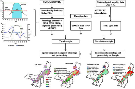
The Global Inventory Modeling and Mapping Studies (GIMMS) 15-day composite NDVI3g dataset with an 8 km spatial resolution applied here has been shown to be more accurate than the GIMMS NDVI for monitoring vegetation activity and phenological change [33]. Data were derived from the AVHRR instrument on board the NOAA satellite series (7, 9, 11, 14, 16–19) for the time period of July 1981 to December 2013. These data had been corrected for calibration, solar geometry, heavy aerosols, clouds, and other effects not related to vegetation change with flag information [34]. If the flag shows 1, 2, or 7, it represents a good value or missing data, respectively. Other flag values mean that NDVI was retrieved from different methods [35]. Although GIMMS NDVI3g data has limitations, it is the longest time series of NDVI for monitoring the characterization and variability of vegetation. The dataset was directly downloaded from the NASA website [35]. For each pixel, the GIMMS NDVI3g time series dataset was pre-processed using the Savitzky-Golay Filter to smooth NDVI with erroneous spikes due to clouds [36].
2.2.2. Drought Index and Meteorological Data
As a site-specific drought indicator, SPEI is particularly suited to detecting, monitoring, and exploring the consequences of global warming on drought conditions [37]. It is formulated based on precipitation and potential evapotranspiration (PET) [31,32]. Different SPEIs are obtained for different time-scales representing the cumulative water balance over the previous several months [15]. To calculate SPEI at different scales, we collected mean monthly air temperature and total monthly precipitation data during the period 1982–2012 from the China Meteorological Data Sharing Service System [38]. Some missing data in the specific stations were replaced by linear regression estimation according to the closest series.
Here, three-month scale and 12-month scale SPEI values were calculated at 116 weather stations via the SPEI Calculator (SPEI calc) [39,40]). We chose the three-month scale SPEI from May as the spring drought index (SPEI_May) and from October as the autumn drought index (SPEI_Oct), and the 12-month scale SPEI value from December as the annual drought index (SPEI_year). Based on the categorization of dryness/wetness grade by SPEI [41], drought is defined as when SPEI was less than −1.0, and wet was defined as greater than 1.0. The normal period was defined as −1.0 < SPEI < 1.0.
All meteorological monthly data were interpolated 8 km spatial resolution grid data based on Partial Thin Plate Smoothing Splines (PTPSS) Models via ANUSPLIN software [42,43]. The interpolation method accuracy of ANUSPLIN is higher than that based on the inverse distance weight method and ordinary Kriging method in China [44]. According to the interpolation, the average signal to noise ratio (SNR) of precipitation, temperature, and SPEI is 0.340, 0.372, and 0.371, respectively, which is smaller than 1. The mean square for error (MSE) of the meteorological elements (precipitation, 0.0012; temperature, 0.0018; SPEI, 0.0065) is less than the generalized cross validation (GCV) value (precipitation, 0.0052; temperature, 0.0055; SPEI, 0.0336). These assessment indicators showed that the PTPSS Models and simulated surface are good for interpolating meteorological elements.
2.2.3. Other Auxiliary Data
MODIS IGBP land cover data (MCD12Q1) with a 500m spatial resolution and 75% accuracy [45] from 2001 to 2012 were analyzed to trace land cover changes and a relatively stable area (Figure S1), where change times are non-zero and zero values, respectively. Then, the stable areas were reclassified into five main classes, including forest, grassland, cropland, shrub, and barren/sparsely vegetated lands (Figure 1b). We extracted the percentage for the five land cover types at 8 km. The largest percentage type was defined as a new type for the 8-km pixel. Additionally, elevation data were derived from the “China Western Environment and Ecology Science Data Center” [46] with a spatial resolution of 1 km, and were resampled into 8 km to interpolate meteorological data via ANUSPLIN.
2.3. Extraction of Phenological Metrics and Vegetation Productivity
Here, the dynamic threshold method and derivative method were selected to extract phenological metrics (e.g., SOS, EOS, LOS) with smoothed GIMMS NDVI3g data, based on previous research and characteristics of the study area [47,48,49,50,51].
2.3.1. Dynamic Threshold Method (m1)
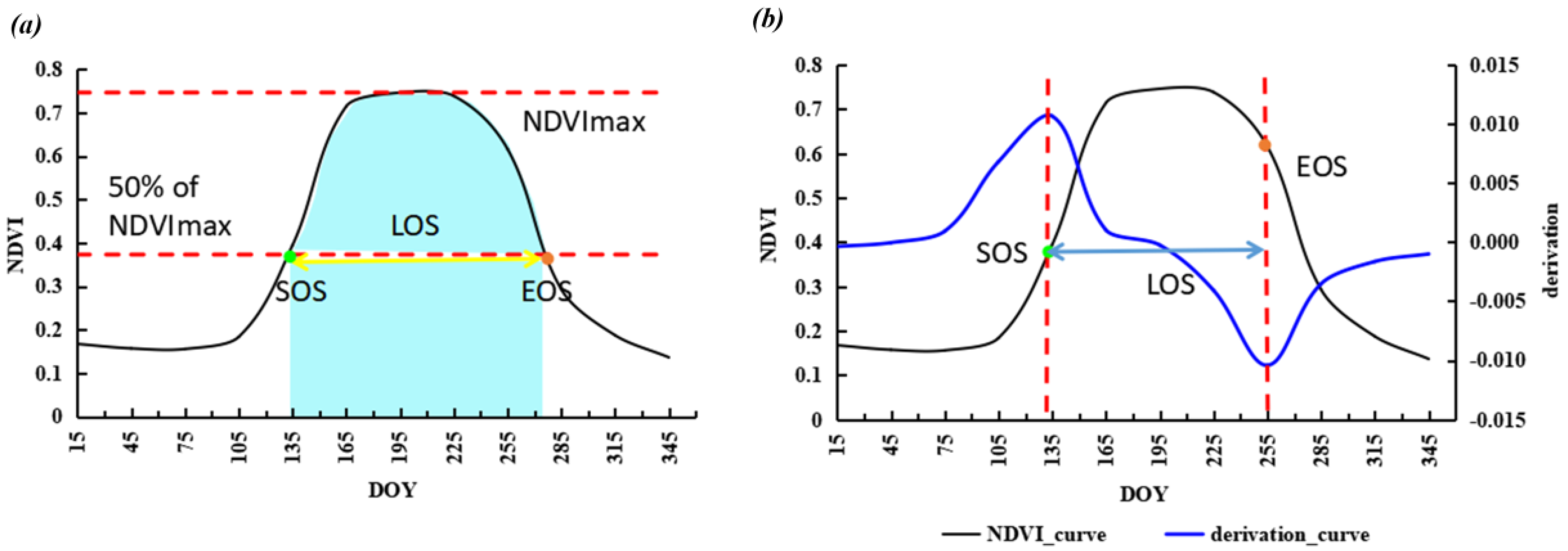
Taking 50% of the maximum NDVI value as the threshold to extract SOS and EOS (Figure 2a) could be reliable for different land cover types in semi-arid regions of China referencing previous studies [48]. LOS was calculated as the difference between SOS and EOS. Finally, the integral value of smoothed NDVI during the growing season (iNDVI) was taken as a proxy of NPP (light blue part in Figure 2a).
2.3.2. Derivative Method Based on the Fitted Double Logistic Function (m2)
The theory of the derivative method is based on the NDVI time series curve and its derivation function to retrieve SOS and EOS. The date of maximum and minimum derivation is SOS and EOS, respectively (Figure 2b) [51]. The Double Logistic function was used for fitting the NDVI time series curve. The fitted equitation is as follows [52,53]:
where NDVImin and NDVImax are the minimum and the maximum NDVI during the growing year season, respectively; S and A are two inflection points, one as the curve rises (S) and one as it drops (A); and ri and rm are the rate of increase or decrease of the curve at the inflection points, respectively.
2.4. Statistics
2.4.1. Trend Analysis
Temporal trends in the datasets were examined by applying the Theil–Sen (TS) median slope trend analysis, which is a robust trend detection method. Functionally similar to linear least squares regression, it operates on non-parametric statistics and is independent of the assumptions of linear regression. Trends are estimated using the median values and are therefore less susceptible to noise and outliers [54,55].
where, xi and xj are the value of the ith or jth year, respectively.
A non-parametric test (Mann-Kendall significance test) was used to test the significance of the TS median slope value, producing z scores and providing information on both the significance and direction of the trend. A positive slope (z ≥ 1.96) represents a significant increase and a negative slope (z ≤ −1.96) indicates a significant decrease (p < 0.05) over time [56].
2.4.2. Correlation Analysis
The anomalies of SOS, EOS, LOS, and iNDVI were calculated to assess the response of phenology and productivity to drought by correlation analysis. Standardized anomalies were calculated by dividing anomalies by the standard deviation:
where, xsd is the standard anomalies of SOS, EOS, LOS, and iNDVI; x is the SOS, EOS, LOS, and iNDVI at any given year; and μ and σ are the mean and standard deviation of SOS, EOS, LOS, and iNDVI during the 1982–2012 time period, respectively.
The slope, p-value and correlation coefficients of the linear regression between anomalies and SPEI were analyzed. All the data processing was finished in IDL 8.3 and ArcGIS 10.2.
3. Results
3.1. Climatic Variation Analysis in Semi-Arid Regions of Northern China
The climatic variation or dry-wet conditions in the study area were characterized by precipitation, temperature, and SPEI values. Four main land cover types, namely: grassland, cropland, barren/sparsely vegetated lands, and shrub, showed a significant warming trend from 1982 to 2012 (Figure S2). Although precipitation has seen no significant trend during the last three decades, the amplitudes of inter-annual variation for grassland and shrub regions were higher than those for cropland and barren/sparsely vegetated lands (Figure S2). For example, precipitation increased abnormally in 1998 for grassland and decreased abnormally in 1991 for shrubland. From the SPEI perspective, grassland (Figure S2b), cropland, and barren or sparsely vegetated lands (Figure S2d) presented a wetter trend during the first 15 years and a drier one for the last 15 years, except for 2010. Annual drought was more severe in 1999, 2000, 2005, and 2009, spring drought in 2000 and 2009, and autumn drought in 1999.
3.2. Spatial-Temporal Patterns of Vegetation Phenology and Productivity
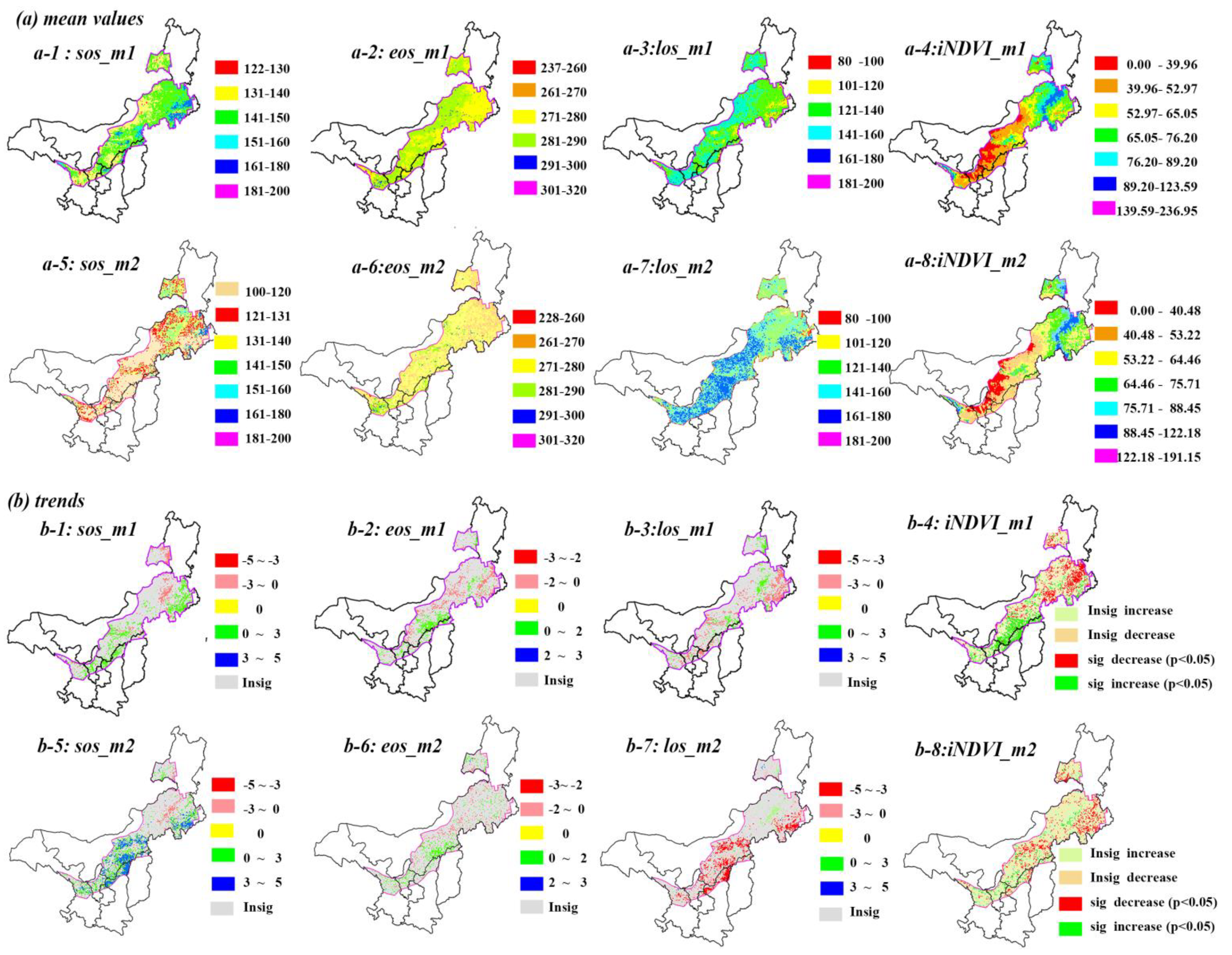
In semi-arid regions, phenology showed different mean values via two different methods. SOS generally falls in the range between DOY 122 and 160 (Figure 3(a-1)) based on the threshold method, whereas it advanced for 10–20 days based on the derivative method (Figure 3(a-5)). Similarly, EOS also advanced for around 10 days via the derivative method, with a range of DOY 260-290 (Figure 3(a-2),(a-6)). Consequently, the retreat of LOS for the derivative method is longer than that for the threshold method in Mu Us Sandy Land and north of Yinshan Mountains due to advanced SOS. LOS ranged from 121 to 180 days in most semi-arid regions (Figure 3(a-3),(a-7)).
Spatial distributions of vegetation phenology, however, are fairly similarly derived from the threshold and derivative method. For instance, late SOS (e.g., after DOY 160) regions mainly surrounded the Horqin Sandy Land. Early EOS (260 < DOY < 280) regions mainly included the whole Horqin Sandy Land, the Da Hinggan Ling Mountains, the Yinshan Mountains, and the middle of the Mu Us Sandy Land, while late EOS has a scattered distribution in the study area (Figure 3(a-2),(a-6)). The iNDVI showed the same spatial patterns over this region. It decreased from east to west, except along the Da Hinggan Ling Mountains (Figure 3(a-4),(a-8)). In contrast, SOS, EOS, LOS, and iNDVI took on more obvious latitude and longitude trends via the threshold method than via the derivation method.
From the perspective of phenology dynamic trends, the results of the two methods were almost consistent, even though the rates of variation show little difference. SOS caused delays of one to five days per decade (1–3 days for m1, 3–5 days for m2, p < 0.05) in the Horqin Sandy Land and the eastern Ordos Plateau. Advanced SOS regions (Figure 3(b-1),(b-4)) were found along the Da Hinggan Ling Mountains with the rate of three to five days per decade (p < 0.05). EOS caused an advance of two days per decade (p < 0.05) in the middle and east of Inner Mongolia, and a delay of two days per decade (p < 0.05) around the junction regions of Inner Mongolia and Shanxi province during 1982-2012 (Figure 3(b-2),(b-4)). The shortened LOS surrounded the Horqin Sandy Land and local places of the Yinshan Mountains. Other regions showed a decreased trend from east to west (Figure 3(b-3),(b-7)), that was similar to the delayed SOS regions (Figure 3(b-1),(b-3)). A significantly decreased area of iNDVI was mostly distributed in the north of semi-arid regions, while in the south of semi-arid regions, such as the Mu Us sandy land and Loess Plateau, an increased trend of iNDVI was found to be significant via the threshold method, and insignificant via the derivation method.
3.3. Response of Phenology and Productivity to Drought
In semi-arid regions, the significant correlations between SOS anomalies to spring drought were almost negative (8.28% for m1, 11.04% for m2, Table 1), and were located in the north of semi-arid regions (Figure 4). These regions, however, were not completely consistent with delayed SOS regions (Figure 3b). The significantly positive responses of EOS to autumn drought were in the southwest and middle-east of the study area and two-sides of the agro-pastoral transition zone, similarly to the EOS delayed or advanced regions (Figure 3b). Compared with EOS, an opposite result was found for LOS. Some shortened growing season length regions did not show a significant correlation with SPEI, e.g., in the region of the Horqin Sandy Land (Figure 3b and Figure 4). Similar to EOS, iNDVI presented a significant positive correlation with SPEI in the north of semi-arid regions, where productivity had an obvious negative trend (Figure 3b and Figure 4). It should be noted that the significantly correlated area of m1 is smaller than that of m2 for SOS, and larger for EOS and iNDVI. The difference between the two methods for correlated patterns of LOS and SPEI is obvious except in the Hulun Buir Sandy Land. However, the sensitivity of phenology and productivity to drought disturbance was consistent based on these two methods. The following relation holds: SOS < LOS < EOS < iNDVI.
3.4. The Phenology and Productivity among Different Land Cover Types
Since there are more obvious latitude and longitude trends of phenology, a more significant iNDVI dynamics area, and a larger correlated area than that of derivation method, the threshold method was chosen to analyze the dynamics of phenology and productivity among different land cover types.
3.4.1. The Spatio-Temporal Trends of Phenology among Different Land Cover Types
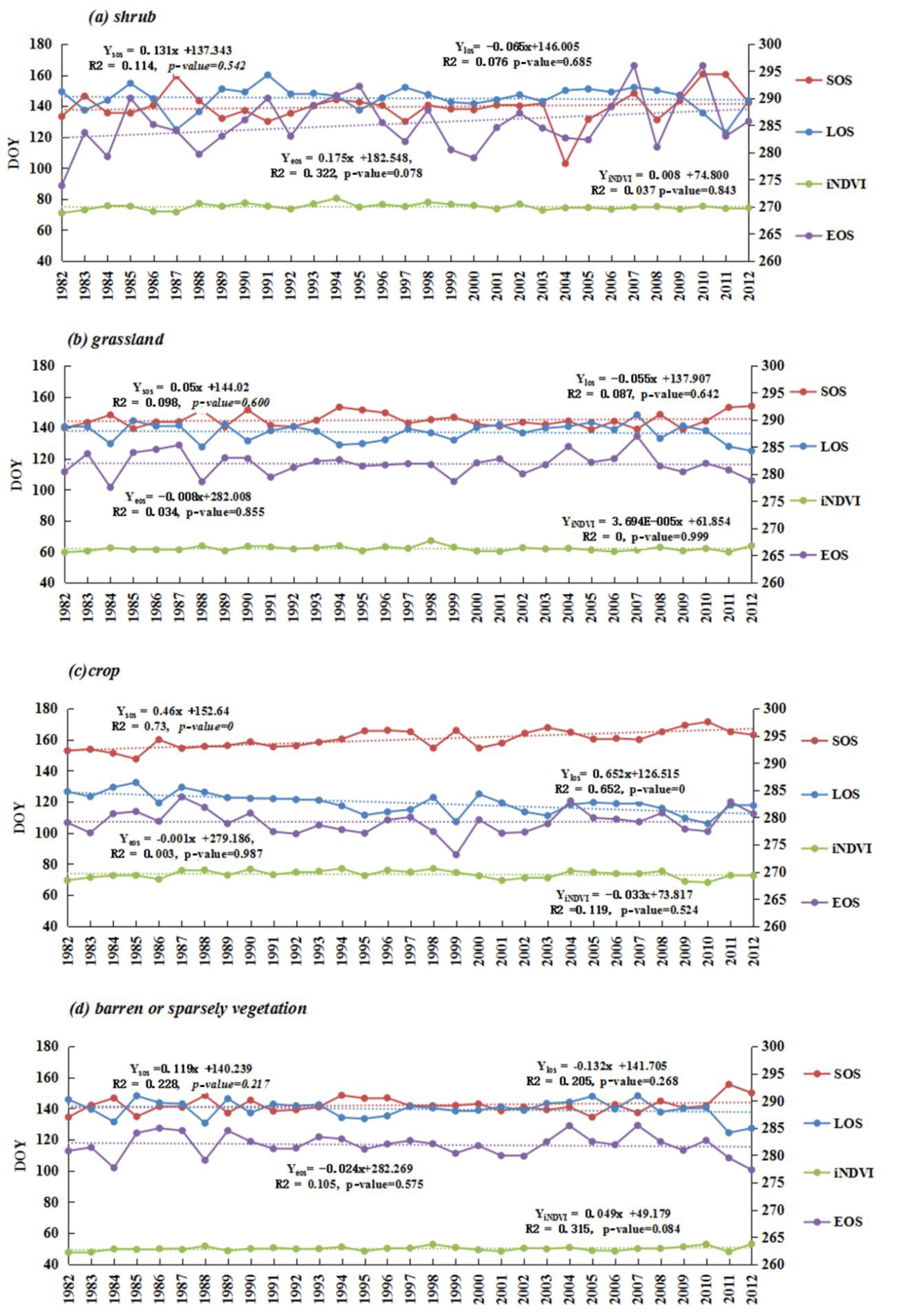
At land cover type stable regions, grassland, shrub, and barren or sparsely vegetated land did not show a significant trend of phenology and iNDVI, except in the case of cropland (Figure 5). Combined with climate analysis, EOS advanced in most autumn drought years at shrub, cropland and barren or sparsely vegetated land, such as in 1999. Grassland and cropland showed that SOS caused a delay in the spring drought years (e.g., in 1994 for grassland, 2001–2004 for cropland) and LOS was shortened in the 1999 drought year (Figure 5, Figure S2). Additionally, most significant changes in the regions of phenology have high chances of land cover variation (Figure 3b, Figure S1).
3.4.2. The Response of Phenology and Productivity among Different Land Cover Types
Among the different land cover types, dramatic heterogeneity phenology parameters (SOS and EOS) with dry-wet conditions were found (Table 2). An insignificant negative correlation between SOS anomaly and SPEI_May presented in grassland, barren/sparsely vegetation, and cropland. EOS anomalies have a significant positive correlation with SPEI_Oct in grassland and barren/sparsely vegetated lands (p < 0.05); LOS has a significant positive correlation with SPEI_ year for grassland (p < 0.05). Similarly, iNDVI also showed a positive correlation with SPEI_year at grassland, shrub, and barren/sparsely vegetated land, and the correlation coefficients are higher than those of LOS (Table 1 and Table 2; Figure 5). This revealed that vegetation productivity presented much more sensitivity than phenology metrics.
4. Discussions
In this study, we analyzed the spatio-temporal changes of vegetation phenology and productivity, and investigated the responses of phenology and productivities to drought disturbance among different land cover types. The results showed that vegetation phenology and productivity have different trends and responses to drought disturbance.
4.1. Spatio-Temporal Trends of Vegetation Phenology and Productivity
Vegetation phenological metrics showed dramatic spatial heterogeneity over the study area, indicating the complicated effects of climate, vegetation, and soil conditions on phenology [17]. Certainly, different methods increase the heterogeneity and uncertainty of phenology. In this study, the trends have fairly similar patterns based on two different methods, even though the rates are slightly different. For instance, the majority of advanced SOS trends occurred along the Da Hinggan Ling Mountains, with a minority occurring along the Yinshan Mountains. Delayed EOS is mainly distributed in the junction regions of Inner Mongolia and Shanxi province (Figure 3b). These results are supported by the conclusions of Wu et al. [17], Cong et al. [57], and Liu et al. [23]. On account of different vegetation types, climatic zones, and water-heat conditions, the positive and negative change trends of phenology have different rates: SOS advanced by three days per decade (p < 0.05), and EOS delayed by two days per decade (p < 0.05) in semi-arid regions of Northern China. These results strongly support previous findings of phenology trends in the Northern Hemisphere [58] and China [59], but the results are lower than in the Inner Mongolia grassland regions [44]. For grassland, advanced EOS was confirmed by Yang et al. [59], whereas phenology variation in shrubland was slightly different than that described by Liu et al. [23]. The positive and negative trend of iNDVI during the growing season based on the threshold method is consistent with the results of Gong et al. [19] and Cao et al. [60]. Hence, compared with the derivative method, the threshold method may be relatively effective for phenology analysis in the semi-arid region of northern China.
4.2. The Responses of Vegetation Phenology and Productivity to Drought
Commonly, temperature and precipitation are widely used to reveal the impacts of climate change on vegetation phenology and productivity [15,16,17,18,19]. Here, focusing on the responses of phenology and productivity to dry-wet conditions based on SPEI, several new insights were obtained by our results. First, drought could explain the anomalies of phenology and productivity (Figure 4). Spring drought delayed SOS and autumn drought significantly advanced EOS, which confirms our assumption and lies in the dynamics of hydrothermal conditions [48]. As we mentioned in introduction, drought shifts the phenology by carbon and water processes [7,11,12]. Due to spring drought, there is not enough available soil water for carbon synthesis during the photosynthesis process, so vegetation grows much more slowly than the normal situation [61,62]. In contrast, on the one hand, autumn drought prompts leaves to close the stoma to decrease the transpiration and photosynthesis rates. On the other hand, respiration maintain higher rates to accelerate carbon degradation, and vegetation starts to stop growing earlier than normal years [62,63]. Similar results also occurred in the cropland/grassland mosaic of North East China Transect [30].
Second, the sensitivity of productivity on drought disturbance is larger than vegetation phenology (Table 1 and Table 2 and Figure 4). Productivity is the direct response to drought, while phenology is the indirect response to drought. It should be noted that the uncertainty of productivity assessment based on NDVI and phenology parameters might overestimate the sensitivity. Additionally, some researches realize the positive correlation between SOS and EOS [64,65]. Nonetheless, it should be noted that the influence of earlier SOS on the determination of EOS was weaker than climatic variables [64,65]. Although we did not take the relationship into consideration for phenology analysis, it has been noted that negative correlations were found in barren/sparsely vegetated land during 1982–2012 (Figure 5).
4.3. Analysis at Different Land Cover Types
The most significant regions of change in phenology occurred not in stable land cover type regions, but in the regions with high chances of land cover variation (Figure 3b, Figure S1). This verifies that land cover is an important factor for phenology change [51]. Significant phenology dynamics in stable cropland may result from human disturbance. Different land cover types showed different responses to drought (Table 2). Because water is the main limiting factor in the grassland of Northern China’s semi-arid regions, grassland showed a much more significant response to drought. In contrast, irrigation could help the phenology of cropland to maintain stable changes.
4.4. Uncertainty Analysis
One of the major uncertainties associated with satellite-derived phenology lies in the different methods. As the results showed, the phenology differences of two methods are obvious (Figure S3). Both mean SOS and EOS advanced by 10 days via the derivative method, compared with the dynamic threshold method (Figure 3a). The SOS values derived by the threshold method and EOS by the derivative method agree with that of Wu et al. [20]. The EOS derived by the threshold method is similar to that of the Double Logistic methods by Liu et al. [57] and that of the Polyfit method by Yang et al. [59]. Due to lack of field investigation data, it is difficult to decide which method is best for different land cover types and different study areas. Fortunately, several researches focus on productivity dynamics. The consistent conclusion is that the vegetation productivity of Mu Us sandy land has significant increased trends [19,66], which agree with our results based on the threshold method. Furthermore, more obvious latitude and longitude trends of the mean values of phenology via the threshold method are related to thermal and hydrological conditions. Therefore, relatively speaking, the dynamic threshold method is much more reliable in the semi-arid region of northern China.
Another uncertainty results from satellite data sources. GIMMS NDVI3g, SPOT-VGT, and MODIS NDVI data are the most commonly used for monitoring phenology [51]. Due to the characteristics of resolution, different NDVI data sources have different accuracies of phenology. Some showed large discrepancies for SOS, comparing GIMMS NDVI 3g NDVI and MODIS NDVI data in Europe [67], equatorial areas, Artic areas, and arid areas [68]. Other research considered that long-term GIMMS data was more accurate than SPOT-4 VGT NDVI [69], showing consistency and strong correlations between GIMMS NDVI3g and MODIS NDVI in the semi-arid West Africa zone [70,71] and China [68]. Furthermore, the coarse time resolution of GIMMS NDVI3g may underestimate the magnitude of phenology variation. Daily data, however, are not sufficient to detect the change accurately enough to match the weather data. Integrated GIMMS NDVI and MODIS NDVI might show spatial heterogeneity for different regions and vegetation types [72], enabling phenology analysis.
Although uncertainties remain, this study has revealed the response of vegetation phenology and productivity to drought. This could be used for ecosystem stability assessment in the future.
5. Conclusions
In semi-arid regions of northern China, the dynamics of vegetation phenology showed dramatic spatial heterogeneity with different rates during the period 1982–2012. Horqin Sandy Land and the eastern Ordos Plateau presented delayed SOS (1–3 days/decade, p < 0.05), and along the Da Hinggan Ling Mountains, advanced SOS was observed (3–5 days/decade, p < 0.05). Advanced EOS (2 days/decade p < 0.05) occurred in the middle and east of Inner Mongolia, while delayed EOS (2 days/decade p < 0.05) was distributed around the junction regions of Inner Mongolia and Shanxi province. Additionally, the significant trends of phenology occurred not in land cover type stable regions, but in the regions with high chances of land cover type variation. In contrast, vegetation productivity presented a clear pattern: in the north of the semi-arid regions there was a significant decrease, while in the south there was a significant increase, particularly in the Mu Us sandy land and Loess Plateau. The response of phenology and productivity to drought was significant and different among land cover types. Spring drought delayed SOS in grassland, barren/sparsely vegetated land, and cropland, while autumn drought significantly advanced EOS in grassland and barren/sparsely vegetated lands. Significant decreased productivity mainly resulted from drought, and the sensitivity of productivity to drought disturbance was larger than that of phenology. These results will be useful for undertaking ecosystem stability assessments in the future.
Supplementary Materials
The following are available online at https://www.mdpi.com/2072-4292/10/5/727/s1. Figure S1: The variation of MODIS land cover types during 2001–2012. Figure S2: Meteorological metrics analysis during 1982–2012 among different land cover types. Figure S3: Comparison phenology metrics between the threshold and derivation method.
Author Contributions
The research was developed and analyzed by W.K.; S.L. and T.W. advised and coordinated the study; the manuscript was written by W.K. with contributions from T.W. and S.L.
Acknowledgments
This study is supported by the Project of National Key Research and Development Program of China, “Assessment on evolution trend and stability of desertified land in the semi-arid region of northern China” (2016YFC0500902).
Conflicts of Interest
The authors declare no conflict of interest.
References
- Poulter, B.; Pederson, N.; Liu, H.; Zhu, Z.; D’Arrigo, R.; Ciais, P.; Davi, N.; Frank, D.; Leland, C.; Myneni, R. Recent trends in inner Asian forest dynamics to temperature and precipitation indicate high sensitivity to climate change. Agric. For. Meteorol. 2013, 178, 31–45. [Google Scholar] [CrossRef]
- Liu, Y.; Zhou, Y.; Ju, W.; Wang, S.; Wu, X.; He, M.; Zhu, G. Impacts of droughts on carbon sequestration by China’s terrestrial ecosystems from 2000 to 2011. Biogeosciences 2014, 11, 2583. [Google Scholar] [CrossRef]
- Hu, S.; Mo, X.; Lin, Z. Projections of spatial-temporal variation of drought in north China. Arid Land Geogr. 2015, 38, 239–248. [Google Scholar]
- Huang, J.; Zhai, J.; Jiang, T.; Wang, Y.; Li, X.; Wang, R.; Xiong, M.; Su, B.; Fischer, T. Analysis of future drought characteristics in China using the regional climate model CCLM. Clim. Dyn. 2017, 50, 1–19. [Google Scholar] [CrossRef]
- Stocker, T. Climate Change 2013: The Physical Science Basis: Working Group I Contribution to the Fifth Assessment Report of the Intergovernmental Panel on Climate Change; Cambridge University Press: Cambridge, UK, 2014. [Google Scholar]
- Ni, J. Plant functional types and climate along a precipitation gradient in temperate grasslands, North-East China and south-east Mongolia. J. Arid Environ. 2003, 53, 501–516. [Google Scholar] [CrossRef]
- Van der Molen, M.K.; Dolman, A.J.; Ciais, P.; Eglin, T.; Gobron, N.; Law, B.E.; Meir, P.; Peters, W.; Phillips, O.L.; Reichstein, M.; et al. Drought and ecosystem carbon cycling. Agric. For. Meteorol. 2011, 151, 765–773. [Google Scholar] [CrossRef]
- D’Odorico, P.; Bhattachan, A.; Davis, K.F.; Ravi, S.; Runyan, C.W. Global desertification: Drivers and feedbacks. Adv. Water Resour. 2013, 51, 326–344. [Google Scholar] [CrossRef]
- Huang, L.; He, B.; Chen, A.; Wang, H.; Liu, J.; Lu, A.; Chen, Z. Drought dominates the interannual variability in global terrestrial net primary production by controlling semi-arid ecosystems. Sci. Rep. 2016, 6, 24639. [Google Scholar] [CrossRef] [PubMed]
- Ivits, E.; Horion, S.; Fensholt, R.; Cherlet, M. Drought footprint on european ecosystems between 1999 and 2010 assessed by remotely sensed vegetation phenology and productivity. Glob. Chang. Biol. 2014, 20, 581–593. [Google Scholar] [CrossRef] [PubMed]
- Hu, Z.; Yu, G.; Fan, J.; Wen, X. Effects of drought on ecosystem carbon and water processes: A review at different scales. Prog. Geogr. 2006, 25, 12–20. [Google Scholar]
- Zhao, M.; Running, S.W. Drought-induced reduction in global terrestrial net primary production from 2000 through 2009. Science 2010, 329, 940–943. [Google Scholar] [CrossRef] [PubMed]
- Ma, X.; Huete, A.; Moran, S.; Ponce Campos, G.; Eamus, D. Abrupt shifts in phenology and vegetation productivity under climate extremes. J. Geophys. Res. Biogeosci. 2015, 120, 2036–2052. [Google Scholar] [CrossRef]
- Poulter, B.; Frank, D.; Ciais, P.; Myneni, R.B.; Andela, N.; Bi, J.; Broquet, G.; Canadell, J.G.; Chevallier, F.; Liu, Y.Y. Contribution of semi-arid ecosystems to interannual variability of the global carbon cycle. Nature 2014, 509, 600–603. [Google Scholar] [CrossRef] [PubMed]
- Piao, S.; Wang, X.; Ciais, P.; Zhu, B.; Wang, T.; Liu, J. Changes in satellite-derived vegetation growth trend in temperate and Boreal Eurasia from 1982 to 2006. Glob. Chang. Biol. 2011, 17, 3228–3239. [Google Scholar] [CrossRef]
- Zhou, Y.Z.; Jia, G.S. Precipitation as a control of vegetation phenology for temperate steppes in China. Atmos. Ocean. Sci. Lett. 2016, 9, 162–168. [Google Scholar] [CrossRef]
- Wu, C.; Hou, X.; Peng, D.; Gonsamo, A.; Xu, S. Land surface phenology of China’s temperate ecosystems over 1999–2013: Spatial–temporal patterns, interaction effects, covariation with climate and implications for productivity. Agric. For. Meteorol. 2016, 216, 177–187. [Google Scholar] [CrossRef]
- Wu, X.; Liu, H. Consistent shifts in spring vegetation green-up date across temperate biomes in China, 1982–2006. Glob. Chang. Biol. 2013, 19, 870–880. [Google Scholar] [CrossRef] [PubMed]
- Gong, Z.; Kawamura, K.; Ishikawa, N.; Goto, M.; Wulan, T.; Alateng, D.; Yin, T.; Ito, Y. Modis normalized difference vegetation index (NDVI) and vegetation phenology dynamics in the inner Mongolia grassland. Solid Earth 2015, 6, 1185–1194. [Google Scholar] [CrossRef]
- Piao, S.; Fang, J.; Zhou, L.; Ciais, P.; Zhu, B. Variations in satellite-derived phenology in China’s temperate vegetation. Glob. Chang. Biol. 2006, 12, 672–685. [Google Scholar] [CrossRef]
- Shen, M.; Piao, S.; Cong, N.; Zhang, G.; Jassens, I.A. Precipitation impacts on vegetation spring phenology on the Tibetan Plateau. Glob. Chang. Biol. 2015, 21, 3647–3656. [Google Scholar] [CrossRef] [PubMed]
- Wang, X.; Piao, S.; Ciais, P.; Li, J.; Friedlingstein, P.; Koven, C.; Chen, A. Spring temperature change and its implication in the change of vegetation growth in North America from 1982 to 2006. Proc. Natl. Acad. Sci. USA 2011, 108, 1240–1245. [Google Scholar] [CrossRef] [PubMed]
- Liu, Q.; Fu, Y.H.; Zeng, Z.; Huang, M.; Li, X.; Piao, S. Temperature, precipitation, and insolation effects on autumn vegetation phenology in temperate China. Glob. Chang. Biol. 2016, 22, 644–655. [Google Scholar] [CrossRef] [PubMed]
- Wang, H.; Liu, G.; Li, Z.; Ye, X.; Wang, M.; Gong, L. Impacts of climate change on net primary productivity in arid and semiarid regions of China. Chin. Geogr. Sci. 2015, 26, 35–47. [Google Scholar] [CrossRef]
- Vicente-Serrano, S.M.; Gouveia, C.; Camarero, J.J.; Beguería, S.; Trigo, R.; López-Moreno, J.I.; Azorín-Molina, C.; Pasho, E.; Lorenzo-Lacruz, J.; Revuelto, J. Response of vegetation to drought time-scales across global land biomes. Proc. Natl. Acad. Sci. USA 2013, 110, 52–57. [Google Scholar] [CrossRef] [PubMed] [Green Version]
- Keenan, T.F.; Gray, J.; Friedl, M.A.; Toomey, M.; Bohrer, G.; Hollinger, D.Y.; Munger, J.W.; O’Keefe, J.; Schmid, H.P.; Wing, I.S. Net carbon uptake has increased through warming-induced changes in temperate forest phenology. Nat. Clim. Chang. 2014, 4, 598–604. [Google Scholar] [CrossRef]
- Zhang, X.; Tarpley, D.; Sullivan, J.T. Diverse responses of vegetation phenology to a warming climate. Geophys. Res. Lett. 2007, 34. [Google Scholar] [CrossRef]
- Wang, T.; Song, X.; Yan, C.; Li, S.; Xie, J. Remote sensing analysis on aeolian desertification trends in northern China during 1975–2010. J. Desert Res. 2011, 31, 1351–1356. [Google Scholar]
- Glade, F.E.; Miranda, M.D.; Meza, F.J.; van Leeuwen, W.J. Productivity and phenological responses of natural vegetation to present and future inter-annual climate variability across semi-arid river basins in chile. Environ. Monit. Assess. 2016, 188, 676. [Google Scholar] [CrossRef] [PubMed]
- Tao, F.; Yokozawa, M.; Zhang, Z.; Hayashi, Y.; Ishigooka, Y. Land surface phenology dynamics and climate variations in the north east China transect (NECT), 1982–2000. Int. J. Remote Sens. 2008, 29, 5461–5478. [Google Scholar] [CrossRef]
- Cui, T.; Martz, L.; Guo, X. Grassland phenology response to drought in the Canadian prairies. Remote Sens. 2017, 9, 1258. [Google Scholar] [CrossRef]
- United Nations Environment Programme. World Atlas of Desertification; UNEP: Nairobi, Kenya, 1992. [Google Scholar]
- Miao, L.; Ye, P.; He, B.; Chen, L.; Cui, X. Future climate impact on the desertification in the dry land Asia using AVHRR gimms NDVI3g data. Remote Sens. 2015, 7, 3863–3877. [Google Scholar] [CrossRef]
- Pinzon, J.; Tucker, C. A non-stationary 1981–2012 AVHRR NDVI3g time series. Remote Sens. 2014, 6, 6929–6960. [Google Scholar] [CrossRef]
- Gimms NDVI3g Data. Available online: https://ecocast.arc.nasa.gov/data/pub/gimms/3g.v0/ (accessed on 5 May 2018).
- Chen, J.; Jönsson, P.; Tamura, M.; Gu, Z.; Matsushita, B.; Eklundh, L. A simple method for reconstructing a high-quality ndvi time-series data set based on the savitzky–golay filter. Remote Sens. Environ. 2014, 91, 332–344. [Google Scholar] [CrossRef]
- Vicente-Serrano, S.M.; Beguería, S.; López-Moreno, J.I. A multiscalar drought index sensitive to global warming: The standardized precipitation evapotranspiration index. J. Clim. 2010, 23, 1696–1718. [Google Scholar] [CrossRef]
- China Meteorological Data Sharing Service System. Available online: http://cdc.cma.gov.cn/ (accessed on 5 May 2018).
- Liu, S.; Kang, W.; Wang, T. Drought variability in inner mongolia of northern China during 1960–2013 based on standardized precipitation evapotranspiration index. Environ. Earth Sci. 2016, 75, 145. [Google Scholar] [CrossRef]
- Speicalc. Available online: http://digital.csic.es/handle/10261/10002 (accessed on 5 May 2018).
- Yu, M.; Li, Q.; Hayes, M.J.; Svoboda, M.D.; Heim, R.R. Are droughts becoming more frequent or severe in China based on the standardized precipitation evapotranspiration index: 1951–2010? Int. J. Climatol. 2014, 34, 545–558. [Google Scholar] [CrossRef]
- Hutchinson, M.F.; Xu, T. Anusplin Version 4.2 User Guide; The Australian National University: Canberra, Australia, 2004. [Google Scholar]
- Liu, Z.; Li, L.; McVicar, T.; Van Niel, T.; Yang, Q.; Li, R. Introduction of the professional interpolation software for meteorology data: Anusplin. Meteorol. Mon. 2008, 34, 92–100. [Google Scholar]
- Qian, Y.; Lv, H.; Zhang, Y. Application and assessment of spatial interpolation method on daily meteorological elements based on anusplin software. J. Meteorol. Environ. 2010, 26, 7–15. [Google Scholar]
- Friedl, M.A.; Sulla-Menashe, D.; Tan, B.; Schneider, A.; Ramankutty, N.; Sibley, A.; Huang, X. Modis collection 5 global land cover: Algorithm refinements and characterization of new datasets. Remote Sens. Environ. 2010, 114, 168–182. [Google Scholar] [CrossRef]
- China Western Environment and Ecology Science Data Center. Available online: http://westdc.westgis.ac.cn (accessed on 5 May 2018).
- Jonsson, P.; Eklundh, L. Seasonality extraction by function fitting to time-series of satellite sensor data. IEEE Trans. Geosci. Remote Sens. 2002, 40, 1824–1832. [Google Scholar] [CrossRef]
- Hou, X.; Niu, Z.; Gao, S.; Huang, N. Monitoring vegetation phenology in farming-pastoral zone using SPOT-VGT NDVI data. Trans. Chin. Soc. Agric. Eng. 2013, 29, 142–150. [Google Scholar]
- White, M.A.; Thornton, P.E.; Running, S.W. A continental phenology model for monitoring vegetation responses to interannual climatic variability. Glob. Biogeochem. Cycles 1997, 11, 217–234. [Google Scholar] [CrossRef]
- Sakamoto, T.; Yokozawa, M.; Toritani, H.; Shibayama, M.; Ishitsuka, N.; Ohno, H. A crop phenology detection method using time-series modis data. Remote Sens. Environ. 2005, 96, 366–374. [Google Scholar] [CrossRef]
- Fan, D.; Zhao, X.; Zhu, W.; Zheng, Z. Review of influencing factors of accuracy of plant phenology monitoring based on remote sensing data. Prog. Geogr. 2016, 35, 304–319. [Google Scholar]
- Beck, P.S.; Atzberger, C.; Høgda, K.A.; Johansen, B.; Skidmore, A.K. Improved monitoring of vegetation dynamics at very high latitudes: A new method using modis NDVI. Remote Sens. Environ. 2006, 100, 321–334. [Google Scholar] [CrossRef]
- Yu, L.; Liu, T.; Bu, K.; Yan, F.; Yang, J.; Chang, L.; Zhang, S. Monitoring the long term vegetation phenology change in northeast China from 1982 to 2015. Sci. Rep. 2017, 7, 14770. [Google Scholar] [CrossRef] [PubMed]
- Sen, P.K. Estimates of the regression coefficient based on kendall’s tau. J. Am. Stat. Assoc. 1968, 63, 1379–1389. [Google Scholar] [CrossRef]
- Theil, H. A rank-invariant method of linear and polynomial regression analysis. In Henri Theil’s Contributions to Economics and Econometrics; Springer: Berlin, Germany, 1992; pp. 345–381. [Google Scholar]
- Fensholt, R.; Rasmussen, K.; Kaspersen, P.; Huber, S.; Horion, S.; Swinnen, E. Assessing land degradation/recovery in the African sahel from long-term earth observation based primary productivity and precipitation relationships. Remote Sens. 2013, 5, 664–686. [Google Scholar] [CrossRef] [Green Version]
- Cong, N.; Wang, T.; Nan, H.; Ma, Y.; Wang, X.; Myneni, R.B.; Piao, S. Changes in satellite-derived spring vegetation green-up date and its linkage to climate in China from 1982 to 2010: A multimethod analysis. Glob. Chang. Biol. 2013, 19, 881–891. [Google Scholar] [CrossRef] [PubMed]
- Zhao, J.; Zhang, H.; Zhang, Z.; Guo, X.; Li, X.; Chen, C. Spatial and temporal changes in vegetation phenology at middle and high latitudes of the northern hemisphere over the past three decades. Remote Sens. 2015, 7, 10973–10995. [Google Scholar] [CrossRef]
- Yang, Y.; Guan, H.; Shen, M.; Liang, W.; Jiang, L. Changes in autumn vegetation dormancy onset date and the climate controls across temperate ecosystems in China from 1982 to 2010. Glob. Chang. Biol. 2015, 21, 652–665. [Google Scholar] [CrossRef] [PubMed]
- Cao, L.; Xu, J.; Chen, Y.; Li, W.; Yang, Y.; Hong, Y.; Li, Z. Understanding the dynamic coupling between vegetation cover and climatic factors in a semiarid region-a case study of inner Mongolia, China. Ecohydrology 2013, 6, 917–926. [Google Scholar] [CrossRef]
- Hinckley, T.; Dougherty, P.; Lassoie, J.; Roberts, J.; Teskey, R. A severe drought: Impact on tree growth, phenology, net photosynthetic rate and water relations. Am. Midl. Nat. 1979, 102, 307–316. [Google Scholar] [CrossRef]
- Chapin, F.S.; Maston, P.; Mooney, H.A. Principles of Terrestrial Ecosystem; Higher Education Press: Beijing, China, 2005; pp. 168–183. [Google Scholar]
- Xu, Z.; Zhou, G.; Shimizu, H. Plant responses to drought and rewatering. Plant Signal. Behav. 2010, 5, 649–654. [Google Scholar] [CrossRef] [PubMed]
- Liu, Q.; Fu, Y.H.; Zhu, Z.; Liu, Y.; Liu, Z.; Huang, M.; Janssens, I.A.; Piao, S. Delayed autumn phenology in the northern hemisphere is related to change in both climate and spring phenology. Glob. Chang. Biol. 2016, 22, 3702–3711. [Google Scholar] [CrossRef] [PubMed]
- Keenan, T.F.; Richardson, A.D. The timing of autumn senescence is affected by the timing of spring phenology: Implications for predictive models. Glob. Chang. Biol. 2015, 21, 2634–2641. [Google Scholar] [CrossRef] [PubMed]
- Yao, Y.; Wang, X.; Li, Y.; Wang, T.; Shen, M.; Du, M.; He, H.; Li, Y.; Luo, W.; Ma, M. Spatiotemporal pattern of gross primary productivity and its covariation with climate in China over the last thirty years. Glob. Chang. Biol. 2017, 24, 184–196. [Google Scholar] [CrossRef] [PubMed]
- Atzberger, C.; Klisch, A.; Mattiuzzi, M.; Vuolo, F. Phenological metrics derived over the european continent from NDVI3g data and modis time series. Remote Sens. 2013, 6, 257–284. [Google Scholar] [CrossRef]
- Fensholt, R.; Proud, S.R. Evaluation of earth observation based global long term vegetation trends—Comparing gimms and modis global NDVI time series. Remote Sens. Environ. 2012, 119, 131–147. [Google Scholar] [CrossRef]
- Fensholt, R.; Nielsen, T.T.; Stisen, S. Evaluation of AVHRR pal and gimms 10-day composite NDVI time series products using spot-4 vegetation data for the African continent. Int. J. Remote Sens. 2006, 27, 2719–2733. [Google Scholar] [CrossRef]
- Schucknecht, A.; Erasmi, S.; Niemeyer, I.; Matschullat, J. Assessing vegetation variability and trends in north-eastern Brazil using AVHRR and modis NDVI time series. Eur. J. Remote Sens. 2013, 46, 40–59. [Google Scholar] [CrossRef]
- Fensholt, R.; Rasmussen, K.; Nielsen, T.T.; Mbow, C. Evaluation of earth observation based long term vegetation trends—Intercomparing NDVI time series trend analysis consistency of sahel from avhrr gimms, terra modis and spot vgt data. Remote Sens. Environ. 2009, 113, 1886–1898. [Google Scholar] [CrossRef]
- Mao, D.; Wang, Z.; Luo, L.; Ren, C. Integrating AVHRR and modis data to monitor NDVI changes and their relationships with climatic parameters in northeast China. Int. J. Appl. Earth Obs. Geoinf. 2012, 18, 528–536. [Google Scholar] [CrossRef]
Figure 1.
Background information of study area. (a) location and elevation; (b) land cover types; (c) mean annual precipitation during 1982–2012; (d) mean annual temperature during 1982–2012.
Figure 1.
Background information of study area. (a) location and elevation; (b) land cover types; (c) mean annual precipitation during 1982–2012; (d) mean annual temperature during 1982–2012.
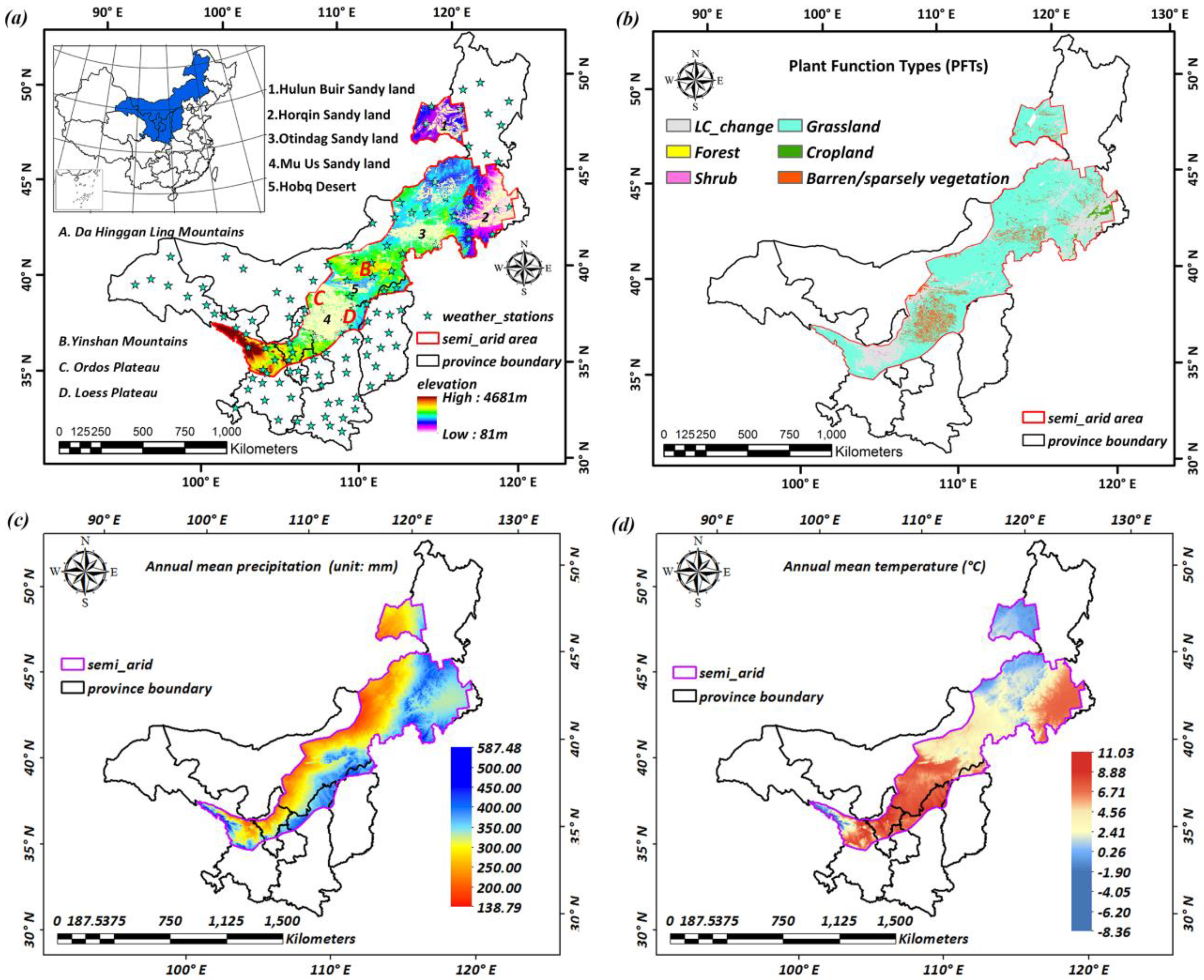
Figure 2.
Diagram of algorithm for deriving phenological metrics and Net Primary Productivity (NPP) proxy. (a) is the algorithm of Dynamic Threshold Method, (b) is the algorithm of Derivative Method.
Figure 2.
Diagram of algorithm for deriving phenological metrics and Net Primary Productivity (NPP) proxy. (a) is the algorithm of Dynamic Threshold Method, (b) is the algorithm of Derivative Method.

Figure 3.
Phenology and productivity average values and spatio-temporal trends based on two different methods. Note, m1 is threshold method, m2 is derivation methods, (a) is the mean value of phenology and iNDVI during 1982–2012, (b) is the temporal trends of phenology and iNDVI during 1982–2012. The unit for phenology mean values and trends are day or days per decade, respectively.

Figure 4.
The correlation coefficients and p-values between phenological metrics, productivity, and SPEI, (a,b) is based on m1 and m2, respectively.
Figure 4.
The correlation coefficients and p-values between phenological metrics, productivity, and SPEI, (a,b) is based on m1 and m2, respectively.

Figure 5.
Phenology and productivity analysis among different land cover types based on threshold method. (a–d) represent shrub, grassland, cropland and barren/sparsely vegetated land.
Figure 5.
Phenology and productivity analysis among different land cover types based on threshold method. (a–d) represent shrub, grassland, cropland and barren/sparsely vegetated land.

Table 1.
Statistical results of significantly correlated area between phenological metrics, productivity, and SPEI based on threshold and derivation methods.
Table 1.
Statistical results of significantly correlated area between phenological metrics, productivity, and SPEI based on threshold and derivation methods.
| Dependent Variables | Independent Variables | Sig Negative (p < 0.05) | Sig Positive (p < 0.05) | Total (p < 0.05) | |||
|---|---|---|---|---|---|---|---|
| m1 | m2 | m1 | m2 | m1 | m2 | ||
| SOS anomaly | SPEI-May | 8.28% | 11.04% | 2.00% | 4.48% | 10.28% | 15.52% |
| EOS anomaly | SPEI-Oct | 0.27% | 1.19% | 18.16% | 7.03% | 18.43% | 8.22% |
| LOS anomaly | SPEI_year | 10.45% | 8.07% | 4.78% | 3.92% | 15.23% | 11.99% |
| iNDVI anomaly | SPEI_year | 0.03% | 0.44% | 37.85% | 7.53% | 37.88% | 7.97% |
Table 2.
Correlation coefficient between anomalies of SOS, EOS, LOS, iNDVI, and SPEI among different land cover types.
Table 2.
Correlation coefficient between anomalies of SOS, EOS, LOS, iNDVI, and SPEI among different land cover types.
| Grassland | Shrub | Barren/Sparsely Veg | Cropland | |||||||
|---|---|---|---|---|---|---|---|---|---|---|
| Dependent Variables | Independent Variables | r | p-Value | r | p-Value | r | p-Value | r | p-Value | |
| SOS anomaly | SPEI-May | −0.04 | 0.85 | 0.14 | 0.44 | −0.16 | 0.50 | −0.05 | 0.78 | |
| EOS anomaly | SPEI-Oct | 0.19 * | 0.03 | 0.14 | 0.27 | 0.31 * | 0.06 | 0.25 | 0.18 | |
| LOS anomaly | SPEI_year | 0.41 * | 0.02 | 0.19 | 0.32 | 0.28 | 0.12 | 0.27 | 0.14 | |
| iNDVI anomaly | SPEI_year | 0.54 * | 0.00 | 0.34 * | 0.05 | 0.36 * | 0.04 | 0.32 | 0.07 | |
Note: ‘*’ means the relationship is significant at 95% confidence level.
© 2018 by the authors. Licensee MDPI, Basel, Switzerland. This article is an open access article distributed under the terms and conditions of the Creative Commons Attribution (CC BY) license (http://creativecommons.org/licenses/by/4.0/).
Share and Cite
MDPI and ACS Style
Kang, W.; Wang, T.; Liu, S. The Response of Vegetation Phenology and Productivity to Drought in Semi-Arid Regions of Northern China. Remote Sens. 2018, 10, 727. https://doi.org/10.3390/rs10050727
AMA Style
Kang W, Wang T, Liu S. The Response of Vegetation Phenology and Productivity to Drought in Semi-Arid Regions of Northern China. Remote Sensing. 2018; 10(5):727. https://doi.org/10.3390/rs10050727
Chicago/Turabian StyleKang, Wenping, Tao Wang, and Shulin Liu. 2018. "The Response of Vegetation Phenology and Productivity to Drought in Semi-Arid Regions of Northern China" Remote Sensing 10, no. 5: 727. https://doi.org/10.3390/rs10050727
Note that from the first issue of 2016, this journal uses article numbers instead of page numbers. See further details here.