Article

Is Ocean Reflectance Acquired by Citizen Scientists Robust for Science Applications?

1
Department of Mathematics and Statistics, University of Victoria, Victoria, BC V8W 2Y2, Canada
2
Department of Geography, University of Victoria, Victoria, BC V8W 2Y2, Canada
*
Author to whom correspondence should be addressed.
Remote Sens. 2018, 10(6), 835; https://doi.org/10.3390/rs10060835
Submission received: 2 May 2018 / Revised: 18 May 2018 / Accepted: 24 May 2018 / Published: 26 May 2018
(This article belongs to the Special Issue Citizen Science and Earth Observation II)

Abstract

:
Monitoring the dynamics of the productivity of ocean water and how it affects fisheries is essential for management. It requires data on proper spatial and temporal scales, which can be provided by operational ocean colour satellites. However, accurate productivity data from ocean colour imagery is only possible with proper validation of, for instance, the atmospheric correction applied to the images. In situ water reflectance data are of great value due to the requirements for validation and reflectance is traditionally measured with the Surface Acquisition System (SAS) solar tracker system. Recently, an application for mobile devices, “HydroColor”, was developed to acquire water reflectance data. We examined the accuracy of the water reflectance measures acquired by HydroColor with the help of both trained and untrained citizens, under different environmental conditions. We used water reflectance data acquired by SAS solar tracker and by HydroColor onboard the BC ferry Queen of Oak Bay from July to September 2016. Monte Carlo permutation F tests were used to assess whether the differences between measurements collected by SAS solar tracker and HydroColor with citizens were significant. Results showed that citizen HydroColor measurements were accurate in red, green, and blue bands, as well as red/green and red/blue ratios under different environmental conditions. In addition, we found that a trained citizen obtained higher quality HydroColor data especially under clear skies at noon.

Graphical Abstract

1. Introduction

Improved understanding of the long-term spatio-temporal productivity of coastal oceans is of fundamental importance for the management of natural resources, especially fisheries [1]. However, the scale of ocean productivity data is generally poor due to constraints related to research ship-based data acquisition. Operational ocean colour satellites such as MODIS-AQUA, VIIRS, and Sentinel-3 can provide data at the required scale; however, data validation is required [2,3]. These satellites measure water reflectance at different wavelengths, which is the basis for the models used to derive concentration of chlorophyll, a proxy for the ocean’s productivity [4]. Limitations on the use of satellite-derived reflectance measurements to retrieve accurate chlorophyll concentrations exist [5]. These limitations are generally a function of inaccurate atmospheric correction of the satellite measured signal and consequently inability to relate this signal to chlorophyll concentrations [6,7,8,9].
The successful use of satellite data requires in situ data to validate both the atmospheric correction and the chlorophyll derived concentrations [10]. Validation of atmospheric correction models, generally, makes use of data acquired with the AERONET (atmospheric transmittance data) and AERONET-OC (water reflectance data) sensors, which are globally distributed, but do not offer sufficient data in certain regions [11,12,13]. Specifically, on the west coast of Canada, there is a lack of sufficient in situ water reflectance data for validation of atmospherically corrected imagery [9,14].
A variety of different instrumentations and techniques for measuring in situ water reflectance exists [15,16]. For instance, the Hyperspectral Surface Acquisition System (HyperSAS, Satlantic Inc., Halifax, NS, Canada) is a common instrument used to measure above-water reflectance ( R r s ) [17,18,19], and has been used extensively in the Salish Sea [9,14,20,21,22]. Recently, the Surface Acquisition System (SAS) solar tracker system, which tracks the position of the Sun for an optimal geometry of data acquisition, has also been used on local waters [23]. A disadvantage of these instruments is that they are both relatively expensive, thus making it difficult to acquire ocean reflectance on a large spatial scale. An alternative is to engage the public, or “citizen scientists”, in ocean reflectance data acquisition to improve the spatial and temporal domain of the data [24].
Citizen science generally refers to the participation of non-scientists in a scientific research project [25]. Although the engagement of citizens allows researchers to gain data on a larger scale with less cost, the quality of citizen scientist data could be a concern. Therefore, citizen science data accuracy assessment is first assessed with regards to effectiveness for the scientific framework [26,27,28], with consideration of accuracy based on providing specialized training [28], and statistical solutions for potential biases [29].
Citizen science has been widely used in different fields, predominantly terrestrial projects [27,28,30,31] and a few ocean related projects [32,33,34,35]. With increasing popularity of sensor-equipped (e.g., inclinometer, digital compass, GPS, camera) and programmable mobile devices, many mobile sensing applications have been developed and can be used to acquire water data for scientific research [36]. Presently, there are many useful mobile sensing applications available to citizens, such as: (1) “EyeonWater” (formerly “Citclops”) developed based on the Forel-Ule colour index system for distinguishing the colours of water bodies [37]; (2) “Creek watch” for the public to report the water flow rate and the amount of water trash [38]; (3)“Marine LitterWatch” for monitoring different kinds of trash in the ocean [39]; (4) “Secchi3000” water quality measurement system for measuring the Secchi depth and turbidity [40]; (5) “HydroColor” for monitoring water quality [41]; and (6) “Algal Watch” for evaluating occurrences of algae with both spatial and temporal scales [42]. To the best of our knowledge, EyeonWater, Algal Watch, and Marine LitterWatch have been used for citizen marine data acquisition in published citizen science studies [42,43,44]. In addition, the accuracy of EyeonWater measurements has been demonstrated in controlled laboratory conditions [45] and ocean satellite reflectance [24]. Other than EyeonWater and Algal Watch, the accuracy of the information derived by the public from these applications is still unknown.
We assessed the feasibility of using the HydroColor application to acquire water reflectance data under different environmental conditions with the help of both trained and untrained citizens onboard the British Columbia ferry Queen of Oak Bay across the Salish Sea. This assessment was performed based on the comparison between citizen HydroColor data and SAS solar tracker data acquired simultaneously on the ferry under different time and cloud cover conditions using Monte Carlo permutation F tests. This project can potentially help with providing in situ R r s data for validating atmospheric correction of satellite imagery by increasing the spatial-temporal match-ups between in situ R r s and satellite imagery. This evaluation will allow us to consider expanding HydroColor data acquisition to “fisher scientists”, an initiative of the Salish Sea Marine Survival project and Ocean Networks Canada (https://marinesurvivalproject.com), thus providing data at a larger spatial scale.

2. Methods

2.1. Study Area

Sampling was conducted along the ferry route from Departure Bay, Nanaimo to Horseshoe Bay, West Vancouver in the area of the Salish Sea, west coast of Canada (Figure 1). This ferry route crosses the Strait of Georgia (SoG), which is a wide semi-enclosed sea approximately 220 km in length between the mainland of British Columbia and Vancouver Island [46]. The water productivity of the SoG is profoundly affected by the outflow of the Fraser River, which generally peaks in June [47,48]. Phytoplankton abundance in the SoG varies seasonally, and is generally highest in the spring and followed by a weaker boom in the fall [9,46]. This variability is associated with the Fraser River plume, tidal mixing, wind, and cloud cover [48]. Turbidity in the SoG has been found to be high at the surface, particularly in the spring and summer coinciding with the Fraser River freshet [49]. In this region, measurements of above-water reflectance ( R r s ) at visible and near infra-red wavelengths show a large magnitude range from 0.001 to 0.027 s r 1 at 400–750 nm due to the variable concentrations of water optical constituents [21]. Spectrally, Phillips and Costa [21] have shown that R r s in the SoG is typically low in the blue wavelengths, high in the green, and low again in the red wavelengths, typical of coastal water bodies [50,51,52].

2.2. Dataset

R r s , turbidity, and chlorophyll- α (Chl α ) measurements were acquired along the Queen of Oak Bay ferry route between 1 July and 5 September 2016. R r s was derived from data collected by ferry passengers with the mobile application HydroColor, and an autonomous hyperspectral radiometer system, SAS solar tracker system.

2.2.1. Citizen HydroColor Measurements

Citizen water reflectance data ( R r s , H ) were collected by HydroColor developed by Leeuw and Boss [41], and available on both Android and iOS mobile devices. This application uses the camera to detect the light intensity coming from the water and sky, and then calculates the red, green, and blue reflectance (denoted as R r s , H ( R ) , R r s , H ( G ) , and R r s , H ( B ) , respectively). HydroColor leverages the GPS, compass, and inclinometer in mobile devices to ensure users obtain precise measurements with an azimuth angle of 135 from the Sun and a zenith angle of 40 from the nadir according to the optimal geometry defined by Mobley [53]. For measuring R r s , H , the user takes a photo of an 18% exposure photography grey card, a photo of the sky, and a photo of the water in the correct direction denoted by green arrows (illustrated in Figure 2). These photos are used to derive downward plane irradiance, sky radiance, and water leaving radiance, respectively. From these measurements, water reflectances of red, green, and blue wavelengths are calculated, and turbidity (0-80 NTU), concentration of SPM (g/m 3 ), and the backscattering coefficient in the red spectra (m 1 ) are estimated based on Gordon et al. [54] and Neukermans et al. [55].
HydroColor measurements were acquired from July to September 2016 every Friday to Monday during two ferry routes: morning (8:30–10:10 a.m.) with a solar zenith angle range from 40.5 to 67.6 and noon (12:50–2:30 p.m.) with a solar zenith angle range from 17.4 to 39.3 [56]. Three iPad mini 4 (Apple Inc., Cupertino, CA, USA) tablets with the HydroColor application were used to acquire data, and two 18% photography grey cards were installed on the railing of the ferry deck for photo taking (Figure 3).
As part of the BC Ferries and Parks Canada Coastal Naturalist Program, a biologist (the same person for the entire sampling period), called a Coastal Naturalist (CN), was trained to use the HydroColor application (trained citizen) before working with ferry passengers (FP, untrained citizens). For quality control, only adults (age 18 or older) were invited to collect data. The established protocol was that the CN gave a 25-min presentation prior to inviting FP to collect data, so a minimum level of information was provided to FP (Figure 4). A total of 446 FP were involved in data collection resulting in a total of 1270 HydroColor samples acquired by CN and FP.
HydroColor data and images were first sorted by environmental conditions: (1) cloud cover; and (2) solar zenith (route time); and subsequently by (3) level of training (Table 1). Cloud cover conditions affect the quality of the R r s data because the reflectance of clouds is brighter than the background sky and therefore produces cloud glitter effects [53]. The time effect was considered because, as the solar zenith angle becomes larger, there is less radiance that is backscattered from the ocean water [57]; consequently, a lower reflectance signal is expected to be detected in the morning. Subsequently, HydroColor data were classified into three categories according to photo quality within the white square (Figure 5): perfect, good, and bad. A sample was classified as “perfect” if all three photos (water, sky, and grey card) had no shadows or other contaminants (Figure 5a); as “good” if only one of them was less than 1/3 contaminated (Figure 5b); and as “bad” if more than one photo was contaminated, or if any of the water reflectance values were zero (Figure 5c). Typical reasons for bad photos were: (1) shade covering grey card or water; (2) white foam or sun glint in the water photo; and/or (3) the photo was entirely different from the object, for example a sky image captured for the photo titled “water”. Conditions (1) and (2) are generally considered as main sources of contamination for R r s measurements [41,58,59]. Only perfect and good samples were considered in the statistical analyses.

2.2.2. Autonomous SAS Solar Tracker Measurements

The SAS solar tracker was installed aboard the ferry to obtain precise R r s measurements for comparison with HydroColor. The system was mounted in the front of the upper deck of the vessel to avoid capturing the vessel structure or its shadow in the measurements [23]. This instrument has three sensors to simultaneously acquire high precision hyperspectral measurements of water-surface radiance, L t ( λ ) , sky radiance, L s ( λ ) , and sky irradiance, E s ( λ ) , where λ is the wavelength from 350 to 800 nm, at a 3-nm resolution. The SAS solar tracker automatically adjusts its sensors’ pointing angles to the correct geometry setting with respect to the vessel’s heading angle and the local sun azimuth angle according to Hooker and Morel [60]. Measurements were acquired continuously when the ferry was travelling and the solar zenith angle was less than 60 [56].
The raw SAS solar tracker data were processed by the automated raw data processing software PySciDon [61] in a 90-s interval, and the above-water reflectance R r s , S A S ( λ ) was calculated according to Ruddick et al. [62]:
R r s , S A S ( λ ) = L t ( λ ) ρ s k y L s ( λ ) E s ( λ )
ρ s k y = 0.0256 + 0.00039 W + 0.000034 W 2 , w h e n L s ( 750 ) E s ( 750 ) < 0.05
ρ s k y = 0.0256 , w h e n L s ( 750 ) E s ( 750 ) 0.05
where ρ s k y is the proportion of sky radiance that is reflected off the surface of the water and is dependent on wind speed W, and on the proportion of cloud cover in the sky radiance measurements. A similar approach has been effectively used by other researchers in this region [9,14,21]. The wind speed obtained from the Government of Canada website (http://climate.weather.gc.ca/) was the average of the hourly wind speeds at buoy 46146 (49.340 N 123.730 W), which is near the mainland, and at Entrance Island (49.209 N 123.811 W), near Nanaimo, both, the closest to the ferry route.
To allow statistical comparison with R r s , H , R r s , S A S ( λ ) was convolved into three broader spectral bands (red, green, and blue) using the spectral sensitivity function (SSF) of the iPad:
R r s , S A S ( i ) = λ = 400 800 R r s , S A S ( λ ) S S F i ( λ ) λ = 400 800 S S F i ( λ ) , i = R , G , B ;
where R r s , S A S ( i ) is the water reflectance of the i t h band, i = R , G , B represents red, green, and blue channels, respectively; S S F i ( λ ) is the spectral sensitivity function of the i t h band; and R r s , S A S ( λ ) is the above-water remote sensing reflectance acquired by SAS solar tracker and computed by Equations (1)–(3).
The SSF of the iPad mini 4 was not available from the manufacturer, and therefore the SSF of the iPhone 5 [41] was used instead after examining for interchangeability. HydroColor data acquired with the iPad mini 4 and the iPhone 5 under a clear sky and green water conditions during 11:30 a.m.–12:30 p.m. on 10 October 2016 were compared. The magnitude and variability of mean difference of the R r s , H between these devices were small, particularly for the red band (Table 2). The mean absolute percentage differences of bands were relatively small compared with a similar study, 69%, 67%, and 77% for red, green, and blue respectively [45], which compared the differences of three bands generated by the iPhone 5 camera’s SSF and the CIE1931 two-degree colour matching function. Therefore, we assumed that using the iPhone 5 camera’s sensitivity function as an alternative was acceptable when the actual function was unavailable.

2.3. Statistical Analyses

Data analyses included examinations of: (1) whether environmental conditions and training affect HydroColor photos’ quality; and (2) whether R r s , H is accurate compared to R r s , S A S and, if not, whether R r s , H can be corrected. We used RStudio version 1.0.136 [63] for all analyses.
First, we used contingency tables and Person’s chi-squared tests on the analysis of the quality of HydroColor photos with environmental conditions (cloud cover and sun zenith) and training to obtain a preliminary understanding of citizen data quality and to assess whether these factors were significant. Second, we analysed the qualified R r s , H and R r s , S A S to assess whether the citizen R r s , H was accurate enough for scientific purposes under all environmental conditions. This analysis considered the R r s values for the blue, green and red bands and the ratios of any two bands’ R r s (red/green, blue/green, and red/blue) for both SAS solar tracker (denoted as R r s , S A S ( R / G ) , R r s , S A S ( B / G ) , and R r s , S A S ( R / B ) , respectively) and HydroColor (denoted as R r s , H ( R / G ) , R r s , H ( B / G ) , and R r s , H ( R / B ) , respectively). Band ratios are generally used in ocean colour chlorophyll algorithms, especially the blue/green ratio [8,64]. All bands and band ratios were considered to be independent and identically distributed random variables.
To assess the accuracy of R r s , H , we evaluated the significance level of mean differences between time-matched R r s , H and R r s , S A S . For this analysis, the differences between R r s , H and R r s , S A S was denoted as:
c c d i j k = R r s , S A S , i j k R r s , H , i j k , i = 1 , 2 , 3 , 4 , 5 , 6 ; j = 1 , 2 , 3 , 4 ; k = 1 , , n j
where R r s , S A S , i j k and R r s , H , i j k are the above-water reflectance acquired by SAS solar tracker and HydroColor under the i t h band or ratio and the j t h environmental condition, respectively. The index i = 1 , , 6 represents the red, green, and blue bands and red/green, red/blue, and blue/green band ratios, respectively; index j = 1 , , 6 represents clear sky morning, cloudy morning, overcast morning, clear sky noon, cloudy noon, and overcast noon respectively; and index k represents the sample number of the j t h environmental condition.
For each band or band ratio, we first tested the normality of d i j · , and subsequently a Monte Carlo permutation F test was used to examine whether the mean of d i j · was significantly different to zero under all environmental conditions [65]. The permutation test is a nonparametric statistical test that does not require distributional assumption, for instance, the normal distribution of standard statistical methods [66].
For those bands and band ratios that showed the mean d i j · were significant, we built piecewise models with environmental condition variables (Equation (5)) to correct the R r s , H based on the corresponding R r s , S A S for future HydroColor data acquisition. The correction error was examined by leave-one-out cross-validation method, the idea and algorithm of which are well documented [67,68]. The leave-one-out error we used was root mean squared error, which has the same scale as R r s .
E ( R r s , c o r r e c t e d ) = β 0 + β 1 R r s , H + β 2 C l o u d + β 3 T i m e + β 4 R r s , H × C l o u d + β 5 R r s , H × T i m e
T i m e = 0 , morning 1 , noon ; C l o u d = 0 , clear 1 , cloudy

3. Results

3.1. HydroColor Photos Quality

A total of 1270 HydroColor citizen samples were collected, in which the number classified as perfect, good, and bad samples were 791, 276, and 203, respectively. The distributions of perfect, good, and bad categories versus training, sun zenith, and cloud cover are shown in Table 3, Table 4 and Table 5, respectively.
The training effect was significantly associated with the quality of HydroColor data ( X 2 2 = 236.3, p < 0.001). The CN (trained) acquired a significantly much higher percentage of perfect data than the FP (untrained) (Table 3). We also observed that data acquired at noon (lower sun zenith) showed slightly higher quality than data acquired in the morning (higher sun zenith) (65% versus 58% of the “perfect category”) (Table 4). The association between HydroColor data quality and the time of day was also significant ( X 2 2 = 14.2, p < 0.001). Moreover, the association between HydroColor image quality and cloud cover was significant ( X 4 2 = 48.5, p < 0.001). Table 5 shows that clear conditions had a higher percentage of perfect data than cloudy or overcast conditions. The highest percentage of bad data (28%) was with overcast conditions since most of the R r s , H values (58 samples, 89% of the bad data) were zero with this condition.

3.2. Accuracy and Correction of R r s , H

For the perfect or good categories, R r s , S A S were first matched with the corresponding R r s , H data by time stamps; a total of n = 214 matches were considered in the analysis. Bad category R r s , H were removed from analyses.
The descriptive statistics for matched R r s , S A S and R r s , H show that the mean and standard deviation of all bands of R r s , H were slightly higher than the corresponding statistics of R r s , S A S (Table 6). The range and trend of both R r s , S A S and R r s , H were similar to another study in this region [21].
The nonparametric Monte Carlo permutation F tests were deemed appropriate because the normality tests indicate that the differences between R r s , S A S and R r s , H for the perfect and good category in most bands and band ratios were not normally distributed. Results of the permutation F tests showed that there were no significant differences between the mean difference and zero under any environmental conditions for red, green bands, and the red/green, red/blue ratios, except for the blue band and the blue/green band ratio, which showed that the true mean difference was significant (Table 7). In addition, R r s , H tended to overestimate the R r s signals for all bands compared to R r s , S A S , although the overestimations were low (Table 7). When only perfect category R r s , H were evaluated, the difference of blue band R r s , H and R r s , S A S was not significant; however, the blue/green ratio R r s , H was still significant (Table 8).
Given the statistically significant observed differences between R r s , H and R r s , S A S for the blue/green ratio, a linear model was built to correct R r s , H ( B / G ) based on R r s , S A S ( B / G ) (Equation (6)). The overcast condition was not included in this model because of the low number of samples (n = 1 for noon, n = 0 for morning).
R r s , c o r r e c t e d ( B / G ) = 0.599 + 0.241 R r s , H ( B / G ) + 0.097 C l o u d 0.146 T i m e 0.084 R r s , H ( B / G ) × C l o u d 0.213 R r s , H ( B / G ) × T i m e
T i m e = 0 , morning 1 , noon ; C l o u d = 0 , clear 1 , cloudy
This can also be written as piecewise models, respectively:
R r s , c o r r e c t e d ( B / G ) = 0.453 + 0.028 R r s , H ( B / G ) , c l e a r n o o n 0.550 0.056 R r s , H ( B / G ) , c l o u d y n o o n 0.599 + 0.241 R r s , H ( B / G ) , c l e a r m o r n i n g 0.696 0.157 R r s , H ( B / G ) , c l o u d y m o r n i n g
This linear model was significant ( F 5 , 207 = 16.18, p < 0.001) with a weak adjusted R 2 (0.26). The prediction performance was assessed by the leave-one-out root mean squared error. Results showed that the magnitude of error was small (0.074), but the percentage of this error compared with mean was high (124%). The correction model does solve the underestimation problem in the original R r s , H ( B / G ) with a fairly high improvement rate (42%). However, Figure 6b also shows a horizontal trend for the morning conditions. This discrepancy may be a result of the small sample sizes of these conditions for parameter estimation.

4. Discussion

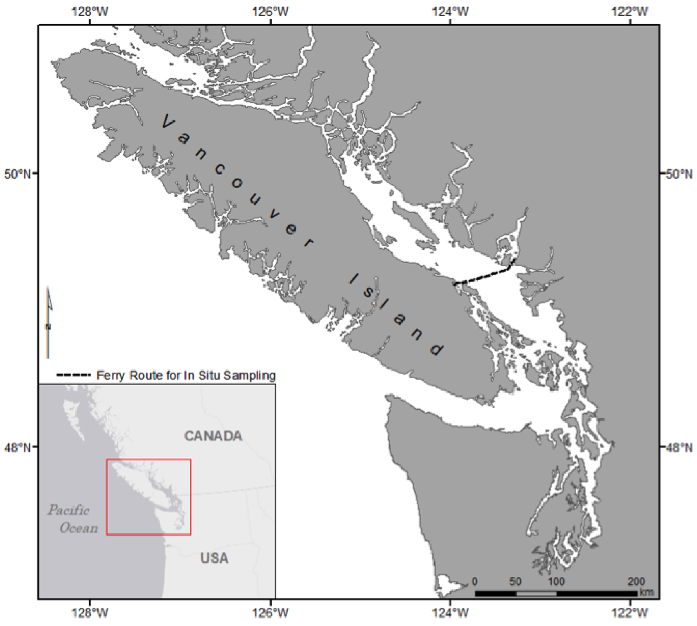
The objective of this study was to examine the accuracy of water reflectance measurements acquired by citizens using the HydroColor application, aiming to provide recommendations for extending the use of Hydrocolor to “fisher scientists”. Although other mobile sensing applications exist, HydroColor is the focus of this research. Water reflectance samples from HydroColor and SAS solar tracker were collected on the BC Ferry Queen of Oak Bay crossing the Strait of Georgia daily, during July to September 2016. The main findings show that the HydroColor citizen data are accurate compared with hyperspectral instrument data for most bands and band ratios; however, citizen level of training and environmental conditions play a role in the data quality.

4.1. Citizen Participation and Data Quality

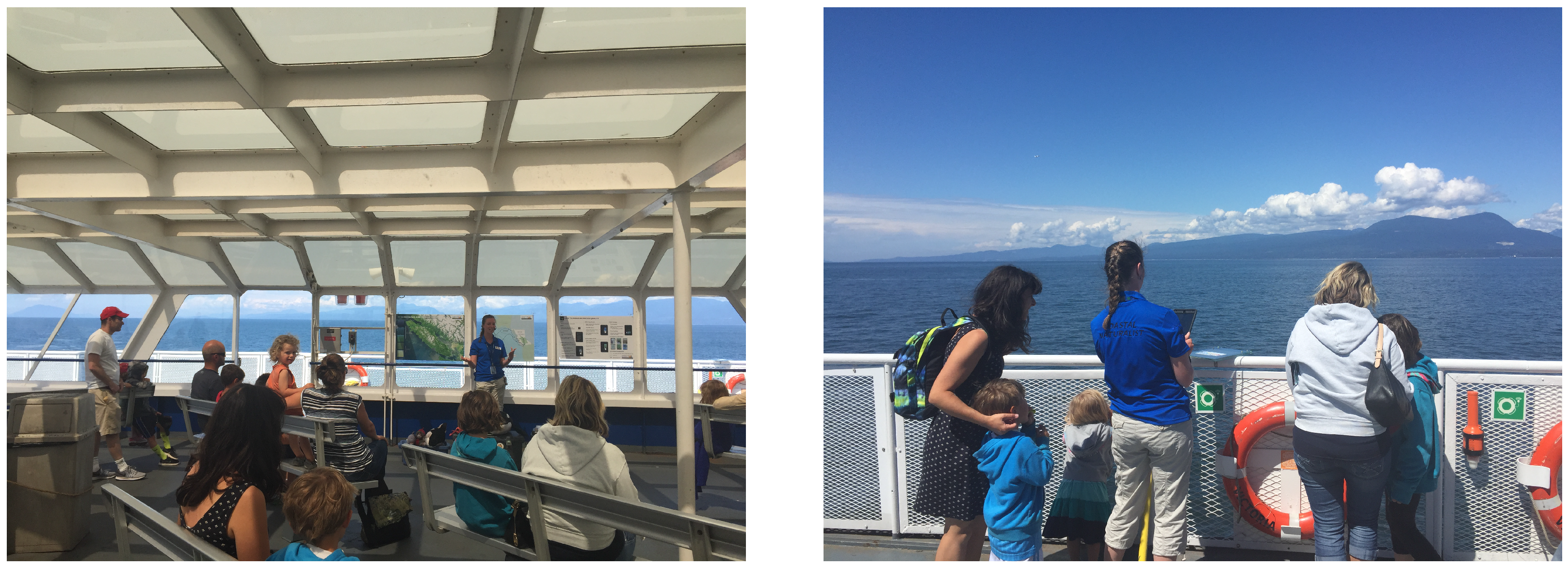
During the study period, which corresponds to the regional tourist season, over 200,000 passengers per month travelled along the ferry route from Departure Bay to Horseshoe Bay (traffic data provided by BC Ferries: http://www.bcferries.com/about/traffic.html). The total number of passengers participating in the data collection was lower than the number attending the educational talk just before the measurements. In addition, the total sample number acquired by regular citizens (FP) was lower than the trained citizen (CN) (Table 3, 446 versus 824). This result suggests that either: (1) volunteer participation for this type of data acquisition may not be as effective, similar to the findings by Kotovirta et al. [42] studying the surface algal bloom citizen monitoring data; or (2) the used methodology prevents larger volunteer participation. The first can be dealt with using an incentive mechanism, such as micro-payments [69]. The second, most likely in this case, could be prevented by having more trained citizens aboard the ferry to help passengers with data acquisition.
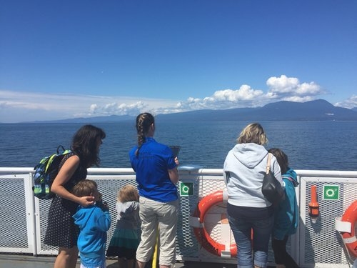
In our methodological framework, only one trained citizen, “the coastal naturalist”, was allowed to guide passengers interested in participating in the experiment (a requirement from BC Ferries). The CN frequently had several people asking questions after the presentation, making it difficult to help all passengers who were willing to acquire data. It would have been useful to have more than one trained citizen (CN) to help with the data collection. In addition, only adults (over age 18) were allowed to participate in data collection. Interestingly, children showed a large interest in using HydroColor for data acquisition, and it would be a valuable experiment to obtain data quality measures for various age groups in future studies.
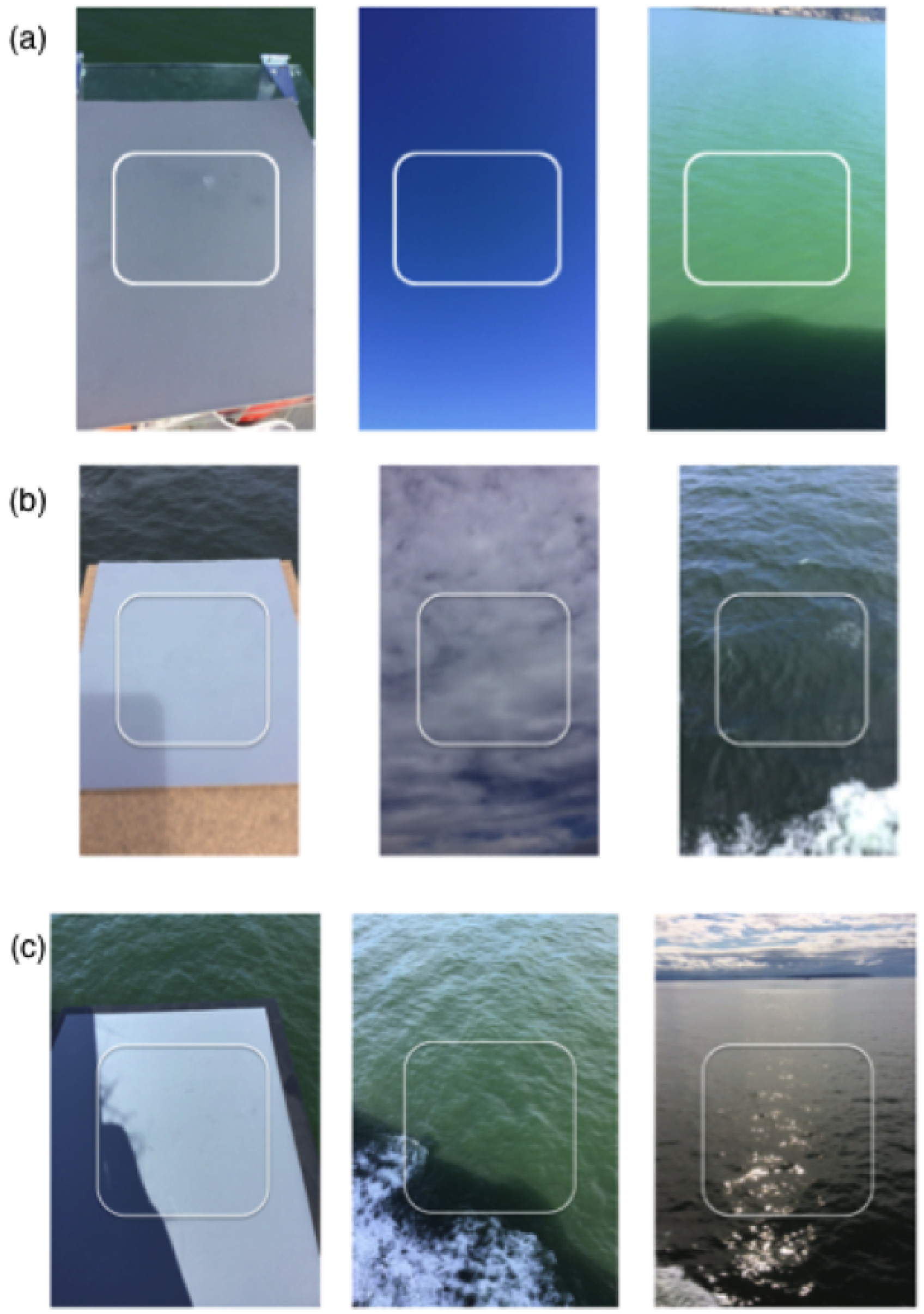
The CN (trained citizen) collected a higher number of samples of higher quality than the passengers (untrained citizen) (77% versus 35%, 
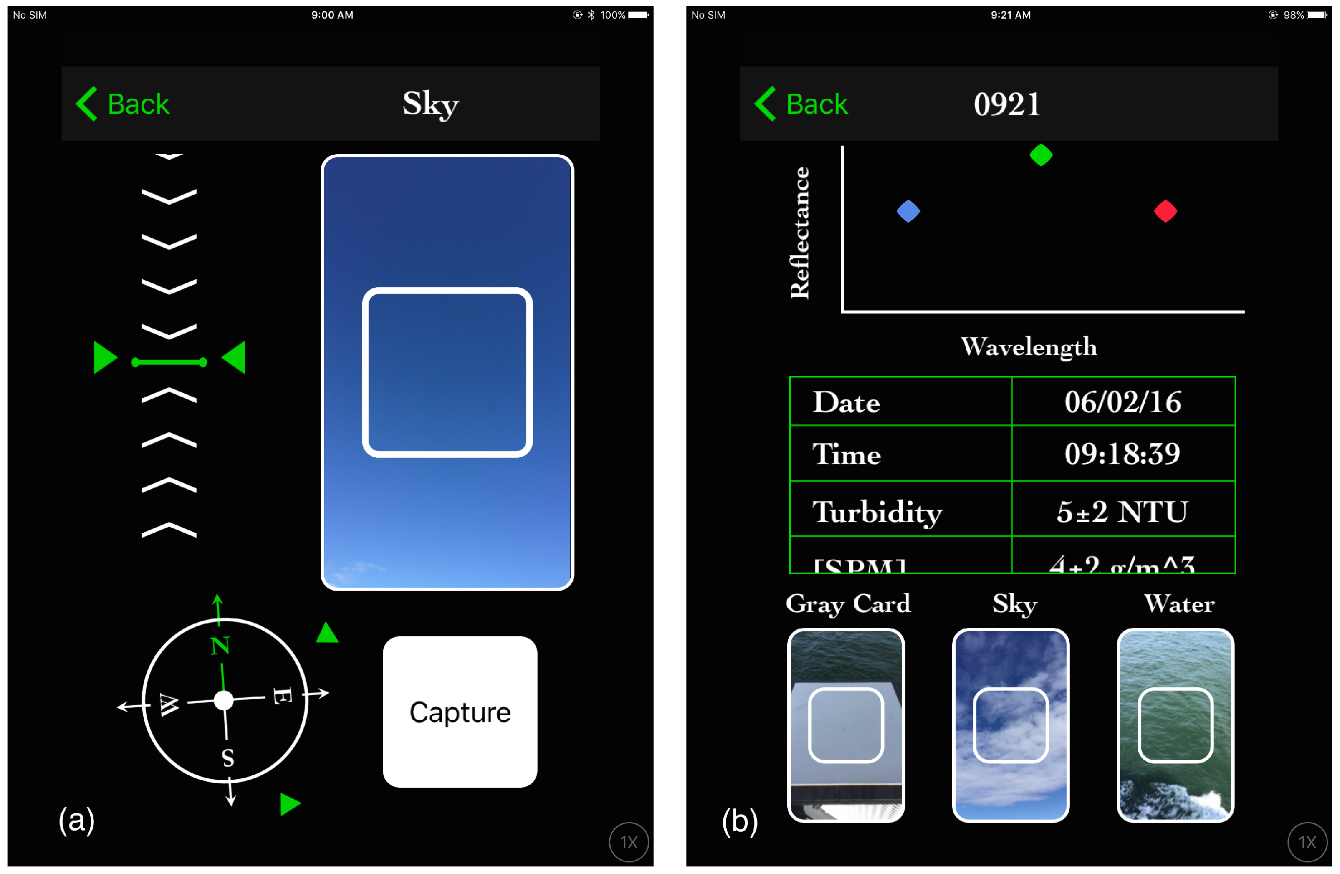
Table 3). This result was not a surprise as the CN had an educational background in environmental science and received training on the use of HydroColor before working on this program. When classifying the untrained citizens’ samples, the main errors were associated with capturing the ship’s shadow and white foam in water photos (Figure 5c). Given the required geometry for data acquisition azimuth angle of 135 from the Sun [41], and the size of the ferry structure, the ship’s shadow and foam are likely to appear in some of the water photos if care is not taken. Focused training such as that given to the CN, can help with improving skills to avoid these errors. The training effect is highly significant (p < 0.001), which implies that a certain degree of training is necessary for high-quality water reflectance sample acquisition using HydroColor. This finding is similar to other studies working with plant species/phenophase [26] and terrestrial invertebrate biodiversity [28]. Volunteers, having around six hours of previous training, could correctly identify 91% of the plant phenophases for a variety of species compared with experts (Fuccillo et al., 2015). The volunteers’ sampling performance for invertebrates, with training in the field, is similar to (p > 0.05) expert researchers [28]. Thiel et al. [34] indicated that appropriate training varies from study to study and should be considered before instructing volunteers.
Besides training, the patience of citizen scientists is also a concern for data quality; for instance, some volunteers did not finish crabs’ size measurements in a study by Delaney et al. [32] since these volunteers thought this process was tedious. In our case, passengers needed the patience to find the correct direction for taking high quality samples. Another approach to improve crowdsourcing data quality suggested by Rogstadius et al. [70] is to emphasize intrinsic motivation such as helping other people.

4.2. Environmental Variables and Data Quality

Similar to many studies [53,57,60,71], our results demonstrated the importance of environmental variables (sun zenith and sky condition) on above-water reflectance ( R r s ) measurement quality. HydroColor data quality was found to be better (p < 0.05) during the noon (time: 12:50–2:30 p.m., solar zenith: 17.4 to 39.3 ) ferry run than the morning (time: 8:30–10:10 a.m., solar zenith: 40.5 to 67.6 ) run (Table 4). A higher percentage of bad samples acquired in the morning (21% versus 13%) was most often due to contamination by the shadow of the ship on the water photos. As sun zenith angle increases, the shadow of the vessel becomes larger and consequently more likely to be detected as part of a sample [71]. In addition to the shadowing effect, the water-leaving radiance is highly related to the time of day or solar zenith [57,72]. Atmospheric attenuation of solar irradiance in the visible and near-infrared spectra decreases as the solar zenith angle decreases [72]. At lower zenith angles, higher irradiance reaches the ocean surface, and therefore more of the water-leaving radiance is detected by the sensor [57]. In our study, morning runs in late August and the beginning of September happened when zenith angles were between 60.0 and 67.6 . At these angles, less irradiance reaches the ocean surface, and consequently less radiance from the water is available for detection by the camera. As a result, it is difficult to detect and calculate satisfactory water reflectance samples in these runs. These findings concur with other studies, showing that a lower sun zenith angle reduces the effects of sun glint, low solar irradiance, weak water-leaving radiance, and wave-shadowing [53,57,71,72].
Sky condition also affected the quality of the data. Higher quality HydroColor data were collected under clear sky conditions than under cloudy and overcast conditions, and the cloudiness effect was significant (p < 0.05, Table 5). This finding is consistent with existing studies recommending a clear sky condition for R r s measurement [53,60,71]. In principle, atmospheric light attenuation in clear sky conditions, mostly due to Raleigh scattering, is relatively more constant than in cloudy or overcast conditions [72]. Further, the reflection of clouds in the water is brighter than the reflectance of blue sky; therefore, more skylight reflected from the water surface was detected by the water-viewing sensor under cloudy conditions [53,71]. Hooker and Morel [60] show that the cloudiness effect is not systematically detected if cloud cover is under a certain threshold. Larger and lower-level cloud cover has a higher effect on the R r s measurements by increasing the magnitude of radiance reflected into the sensor [53].
In addition, to affirm the importance of collecting data under a clear sky, we also found that HydroColor data acquired under overcast conditions were overall the poorest quality; in particular, a relatively large percentage of bad samples (89%) showed water reflectance values equal to zero. This is likely due to the lower sensitivity of the iPad mini 4 camera at low irradiance conditions. This result corroborates the work of Salisbury [72] that illustrated that less measurement radiance signal can be detected under a hazy sky because of blurry shadows, and the work of Garaba and Zielinski [71] that showed that light is more diffuse in hazy skies than clear skies.
Beyond assessing HydroColor data quality, we examined comparisons between HydroColor and the gold standard SAS solar tracker to determine how accurate HydroColor can be as an optical instrument to measure R r s . The evaluation of the accuracy of qualified (classified as perfect and good quality) HydroColor citizen data revealed the larger mean and higher variability (Table 6) for the observed three bands in relation to the SAS solar tracker data ( R r s , S A S ). A possible reason for this result is that different ρ s k y values were used to calculate R r s and R r s , S A S . The ρ s k y is used to remove the proportion of the sky radiance that is reflected off the water surface and detected by the water radiance sensor [53]. In a flat sea surface, the reflected sky radiance can be prescribed by viewing geometry alone, according to the Fresnel reflectance [6]. However, the sea surface is usually wavy due to wind, and therefore the surface reflects sunlight from a range of directions other than only the viewing angle [53]. The ρ s k y value used to calculate R r s , H was set to a constant 0.028 in the HydroColor application [41], while the value used for R r s , S A S was computed by Equations 2 and 3, which is related to wind speed and sky condition. The comparisons of HydroColor data and calibrated Water Insight Spectrometer (WISP) data by Leeuw and Boss [41] does not show that HydroColor tends to overestimate R r s when the same ρ s k y is applied to calculate the above-water reflectance.
According to the results, the observed differences between R r s , H and R r s , S A S for red and green bands were not statistically significant (p > 0.05); however, the difference was significant for the blue band (p < 0.05, Table 7). The result of lower accuracy in the blue band is also shown in the work of Leeuw and Boss [41], which indicates that R r s , H in the blue band has the highest median percent error compared to the WISP among the three bands. Interestingly, when only perfect quality R r s , H was evaluated, the statistical analysis showed that the difference of blue band was no longer significant (p < 0.05, Table 8). These results imply that minor contaminations in the HydroColor photos still introduce errors in the accuracy of the R r s , H for the blue band. The high sensitivity of minor contaminations for the blue band may be caused by: (1) comparably weak blue signals, and therefore subject to more variability due to noise (low signal-to-noise) [73]; (2) relatively high difference and variability between the true spectral sensitivity function and the substitute one; or (3) the fixed ρ s k y programmed in HydroColor, making it difficult to precisely correct the effect of skylight; however, the skylight is mostly contributed by blue band radiance due to Rayleigh scattering [74]. As such, for accurate retrievals of above-water reflectance at the blue spectra using HydroColor, perfect data quality is required.
The average values and variability (Table 7) of the difference between R r s , H and R r s , S A S 
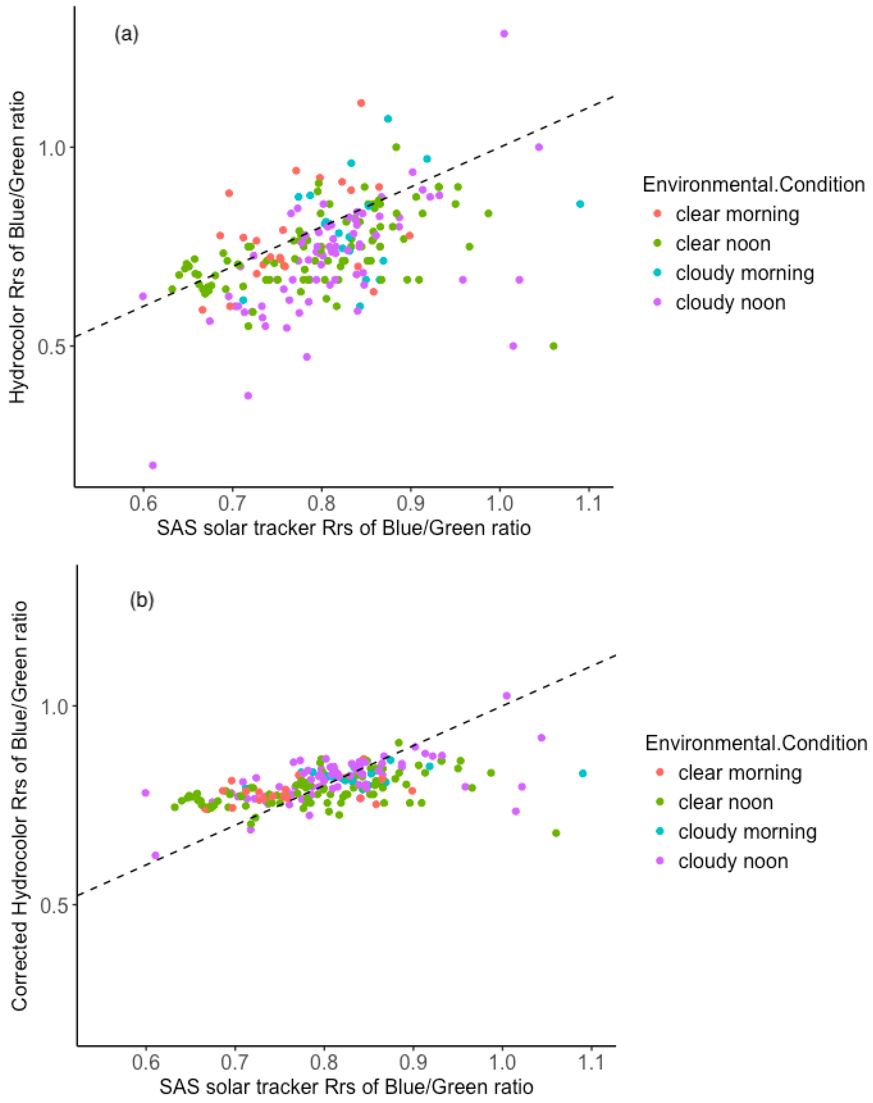
were higher for band ratios than for individual bands. The results of permutation F tests for band ratios (Table 7) showed the difference between R r s , H and R r s , S A S of blue/green ratio was significant (p < 0.05), while the other two ratios were not. The significant differences of the blue/green ratio were first considered as an effect of the bad performance of the blue band with minor contaminations. However, we note that, even discarding samples with contaminations, the significance was not eliminated (p < 0.05, Table 8). Thus, a linear model with environmental factors as variables was developed to correct the bias (Equation 6). Although this correction model was significant (p < 0.05), the low adjusted R 2 (0.26) and the high percentage of correction error (124%) illustrated that it was not satisfactory. Therefore, the magnitudes of individual bands are recommended to be used for scientific purposes rather than band ratios, especially the blue/green ratio. The most likely explanation for this negative finding is that the blue/green band ratio R r s , H 
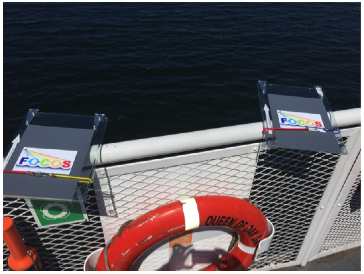
is highly sensitive to the differences between R r s , H and R r s , S A S measurement protocols, which may result in a slight difference in measuring location (different field of view—angle of the lens and different footprint on the water) and time. To clarify, the SAS solar tracker was installed on the same side of the ship where the citizens acquired data, but still at approximately 15 m distance horizontally. In addition, a Hydrocolor sample usually takes one minute to finish collecting the grey card, sky, and water photos, whereas SAS solar tracker collected the data with three sensors simultaneously. Atmospheric properties and water optical constituents are continually changing, and therefore measured reflectance might be slightly different depending on location and time; for instance, clear blue skies with fast cirrus clouds passing in front of the Sun may suddenly change the downwelling irradiance. The studies of Toole et al. [6] and Leeuw and Boss [41] have also mentioned that the deviations between two instruments are partly caused by imperfect matching on time and location.

5. Conclusions

We have conducted the first evaluation of the accuracy of Hydrocolor samples collected by citizens aboard a ferry based on a thorough statistical analysis. We have shown that water reflectance measurements acquired by HydroColor can be used for data acquisition with trained citizen scientists; however, we must be careful when using this method with untrained citizen science. We suggest that oral and written instructions on the use of HydroColor are provided for the “fisher scientists” before asking for their participation in data acquisition. In these instructions, we will recommend that the data should be acquired under clear skies at noon to be high-quality samples. General sources of errors are shadows in the grey card, white foam, shadows, and sun glint in water photos.
We showed that it is acceptable to use the spectral sensitivity function of the iPhone 5 as a substitute for the actual function of the iPad mini 4. Nevertheless, the difference between spectral sensitivity functions was likely a source of error. It would be better to acquire the true spectral sensitivity function of the user device if the “fisher scientists” water reflectance samples need to be compared with ocean colour imagery reflectance in the future.
Future work would include determining the quality of water reflectance samples using HydroColor by “fisher scientists”, especially if the samples will be used as ground-truth data [42]. All images of HydroColor samples in this study were carefully checked for data quality. However, it would be impossible for an individual to check the data with large datasets. Thus, an automated data quality control system should be developed to enhance the reliability of “fisher scientists” data [75].
Systematic citizen science research should provide meaningful citizen involvement as well as use thorough statistical analyses to evaluate the reliability and associated errors of the acquired data [76]. The engagement of citizens not only provides more data needed in natural resource management, but it also closes the gap between scientists and citizens [35].

Author Contributions

M.C. conceived the idea of assessing citizen above-water reflectance data; M.C. and Y.Y. supervised the data collection; L.L.E.C. and Y.Y. constructed the statistical analysis; Y.Y. prepared the original draft; and M.C. and L.L.E.C. reviewed and edited this paper.

Funding

This research was funded by the Marine Environmental Observation, Prediction and Response Network (MEOPAR) and the Pacific Salmon Foundation (PSF)/Salish Sea Marine Survival Project.

Acknowledgments

We would like to thank BC Ferries, Parks Canada and Ocean Networks Canada for their support.

Conflicts of Interest

The authors declare no conflict of interest.

References

  1. Perry, R.I.; Masson, D. An integrated analysis of the marine social–ecological system of the Strait of Georgia, Canada, over the past four decades, and development of a regime shift index. Prog. Oceanogr. 2013, 115, 14–27. [Google Scholar] [CrossRef]
  2. Blondeau-Patissier, D.; Gower, J.F.; Dekker, A.G.; Phinn, S.R.; Brando, V.E. A review of ocean color remote sensing methods and statistical techniques for the detection, mapping and analysis of phytoplankton blooms in coastal and open oceans. Prog. Oceanogr. 2014, 123, 123–144. [Google Scholar] [CrossRef] [Green Version]
  3. Ruddick, K.; Neukermans, G.; Vanhellemont, Q.; Jolivet, D. Challenges and opportunities for geostationary ocean colour remote sensing of regional seas: A review of recent results. Remote Sens. Environ. 2014, 146, 63–76. [Google Scholar] [CrossRef]
  4. Berger, W.; Smetacek, V.; Wefer, G. Ocean productivity and paleoproductivity—An overview. In Productivity of the Ocean: Present and Past; Wiley: New York, NY, USA, 1989; Volume 44, pp. 1–34. [Google Scholar]
  5. Zelenka, A.; Perez, R.; Seals, R.; Renné, D. Effective accuracy of satellite-derived hourly irradiances. Theor. Appl. Climatol. 1999, 62, 199–207. [Google Scholar] [CrossRef]
  6. Toole, D.A.; Siegel, D.A.; Menzies, D.W.; Neumann, M.J.; Smith, R.C. Remote-sensing reflectance determinations in the coastal ocean environment: Impact of instrumental characteristics and environmental variability. Appl. Opt. 2000, 39, 456–469. [Google Scholar] [CrossRef] [PubMed]
  7. Wang, M.; Shi, W. Estimation of ocean contribution at the MODIS near-infrared wavelengths along the east coast of the US: Two case studies. Geophys. Res. Lett. 2005, 32. [Google Scholar] [CrossRef]
  8. Brewin, R.J.; Sathyendranath, S.; Müller, D.; Brockmann, C.; Deschamps, P.Y.; Devred, E.; Doerffer, R.; Fomferra, N.; Franz, B.; Grant, M.; et al. The Ocean Colour Climate Change Initiative: III. A round-robin comparison on in-water bio-optical algorithms. Remote Sens. Environ. 2015, 162, 271–294. [Google Scholar] [CrossRef]
  9. Carswell, T.; Costa, M.; Young, E.; Komick, N.; Gower, J.; Sweeting, R. Evaluation of MODIS-Aqua Atmospheric Correction and Chlorophyll Products of Western North American Coastal Waters Based on 13 Years of Data. Remote Sens. 2017, 9, 1063. [Google Scholar] [CrossRef]
  10. Mueller, J.; Bidigare, R.; Trees, C.; Dore, J.; Karl, D.; Van Heukelem, L. Biogeochemical and bio-optical measurements and data analysis protocols: Ocean optics protocols for satellite ocean color sensor validation. Revision 4, Volume 2. NASA/TM-2003 2003, 21621, 39–64. [Google Scholar]
  11. Franz, B.A.; Bailey, S.W.; Werdell, P.J.; McClain, C.R. Sensor-independent approach to the vicarious calibration of satellite ocean color radiometry. Appl. Opt. 2007, 46, 5068–5082. [Google Scholar] [CrossRef] [PubMed]
  12. Mobley, C.D.; Werdell, J.; Franz, B.; Ahmad, Z.; Bailey, S. Atmospheric Correction for Satellite Ocean Color Radiometry; NASA Goddard Space Flight Center: Greenbelt, MD, USA, 2016. [Google Scholar]
  13. Gilerson, A.; Herrera, E.; Klein, Y.; Foster, R.; Gross, B.; Arnone, R.; Ahmed, S. Characterization of aerosol parameters over ocean from the Ocean Color satellite sensors and AERONET-OC data. Proc. SPIE 2017, 10422. [Google Scholar] [CrossRef]
  14. Komick, N.; Costa, M.; Gower, J. Bio-optical algorithm evaluation for MODIS for western Canada coastal waters: An exploratory approach using in situ reflectance. Remote Sens. Environ. 2009, 113, 794–804. [Google Scholar] [CrossRef]
  15. Ritchie, J.C.; Zimba, P.V.; Everitt, J.H. Remote sensing techniques to assess water quality. Photogramm. Eng. Remote Sens. 2003, 69, 695–704. [Google Scholar] [CrossRef]
  16. Zibordi, G.; Mélin, F.; Berthon, J.F.; Talone, M. In situ autonomous optical radiometry measurements for satellite ocean color validation in the Western Black Sea. Ocean Sci. Discuss. 2014, 11, 3003–3034. [Google Scholar] [CrossRef]
  17. Harmel, T.; Gilerson, A.; Hlaing, S.; Tonizzo, A.; Legbandt, T.; Weidemann, A.; Arnone, R.; Ahmed, S. Long Island Sound Coastal Observatory: Assessment of above-water radiometric measurement uncertainties using collocated multi and hyperspectral systems. Appl. Opt. 2011, 50, 5842–5860. [Google Scholar] [CrossRef] [PubMed]
  18. Hlaing, S.; Gilerson, A.; Harmel, T.; Tonizzo, A.; Weidemann, A.; Arnone, R.; Ahmed, S. Assessment of a bidirectional reflectance distribution correction of above-water and satellite water-leaving radiance in coastal waters. Appl. Opt. 2012, 51, 220–237. [Google Scholar] [CrossRef] [PubMed]
  19. Martinez-Vicente, V.; Simis, S.; Alegre, R.; Land, P.; Groom, S. Above-water reflectance for the evaluation of adjacency effects in Earth observation data: Initial results and methods comparison for near-coastal waters in the Western Channel, UK. J. Eur. Opt. Soc.-Rapid Publ. 2013, 8. [Google Scholar] [CrossRef]
  20. O’Neill, J.D.; Costa, M. Mapping eelgrass (Zostera marina) in the Gulf Islands National Park Reserve of Canada using high spatial resolution satellite and airborne imagery. Remote Sens. Environ. 2013, 133, 152–167. [Google Scholar] [CrossRef]
  21. Phillips, S.R.; Costa, M. Spatial-temporal bio-optical classification of dynamic semi-estuarine waters in western North America. Estuar. Coast. Shelf Sci. 2017, 199, 35–48. [Google Scholar] [CrossRef]
  22. Loos, E.; Costa, M.; Johannessen, S. Underwater optical environment in the coastal waters of British Columbia, Canada. FACETS 2017, 2, 872–891. [Google Scholar] [CrossRef]
  23. Costa, M.; Phillips, S.; Wang, Z.; Vandenberg, N. A road map for autonomous, continuous in situ above-water hyperspectral reflectance data from ferry platforms: Ferry Ocean Colour Observations System (FOCOS). In Proceedings of the International Ocean Optics Conference, Victoria, BC, Canada, 23–28 October 2016; pp. 7–12. [Google Scholar]
  24. Busch, J.A.; Price, I.; Jeansou, E.; Zielinski, O.; van der Woerd, H.J. Citizens and satellites: Assessment of phytoplankton dynamics in a NW Mediterranean aquaculture zone. Int. J. Appl. Earth Obs. Geoinform. 2016, 47, 40–49. [Google Scholar] [CrossRef]
  25. Buytaert, W.; Zulkafli, Z.; Grainger, S.; Acosta, L.; Alemie, T.C.; Bastiaensen, J.; De Bièvre, B.; Bhusal, J.; Clark, J.; Dewulf, A.; et al. Citizen science in hydrology and water resources: Opportunities for knowledge generation, ecosystem service management, and sustainable development. Front. Earth Sci. 2014, 2, 26. [Google Scholar] [CrossRef]
  26. Fuccillo, K.K.; Crimmins, T.M.; de Rivera, C.E.; Elder, T.S. Assessing accuracy in citizen science-based plant phenology monitoring. Int. J. Biometeorol. 2015, 59, 917–926. [Google Scholar] [CrossRef] [PubMed]
  27. Butt, N.; Slade, E.; Thompson, J.; Malhi, Y.; Riutta, T. Quantifying the sampling error in tree census measurements by volunteers and its effect on carbon stock estimates. Ecol. Appl. 2013, 23, 936–943. [Google Scholar] [CrossRef] [PubMed] [Green Version]
  28. Lovell, S.; Hamer, M.; Slotow, R.; Herbert, D. An assessment of the use of volunteers for terrestrial invertebrate biodiversity surveys. Biodivers. Conserv. 2009, 18, 3295. [Google Scholar] [CrossRef]
  29. Bird, T.J.; Bates, A.E.; Lefcheck, J.S.; Hill, N.A.; Thomson, R.J.; Edgar, G.J.; Stuart-Smith, R.D.; Wotherspoon, S.; Krkosek, M.; Stuart-Smith, J.F.; et al. Statistical solutions for error and bias in global citizen science datasets. Biol. Conserv. 2014, 173, 144–154. [Google Scholar] [CrossRef]
  30. Sequeira, A.M.; Roetman, P.E.; Daniels, C.B.; Baker, A.K.; Bradshaw, C.J. Distribution models for koalas in South Australia using citizen science-collected data. Ecol. Evol. 2014, 4, 2103–2114. [Google Scholar] [CrossRef] [PubMed]
  31. Canfield Jr, D.E.; Brown, C.D.; Bachmann, R.W.; Hoyer, M.V. Volunteer lake monitoring: Testing the reliability of data collected by the Florida Lakewatch program. Lake Reserv. Manag. 2002, 18, 1–9. [Google Scholar] [CrossRef]
  32. Delaney, D.G.; Sperling, C.D.; Adams, C.S.; Leung, B. Marine invasive species: Validation of citizen science and implications for national monitoring networks. Biol. Invasions 2008, 10, 117–128. [Google Scholar] [CrossRef]
  33. Hidalgo-Ruz, V.; Thiel, M. Distribution and abundance of small plastic debris on beaches in the SE Pacific (Chile): A study supported by a citizen science project. Mar. Environ. Res. 2013, 87, 12–18. [Google Scholar] [CrossRef] [PubMed]
  34. Thiel, M.; Penna-Díaz, M.A.; Luna-Jorquera, G.; Salas, S.; Sellanes, J.; Stotz, W. Citizen scientists and marine research: Volunteer participants, their contributions, and projection for the future. Oceanogr. Mar. Biol. Annu. Rev. 2014, 52, 257–314. [Google Scholar]
  35. Schläppy, M.L.; Loder, J.; Salmond, J.; Lea, A.; Dean, A.J.; Roelfsema, C.M. Making waves: Marine citizen science for impact. Front. Mar. Sci. 2017, 4, 146. [Google Scholar] [CrossRef]
  36. Lane, N.D.; Miluzzo, E.; Lu, H.; Peebles, D.; Choudhury, T.; Campbell, A.T. A survey of mobile phone sensing. IEEE Commun. Mag. 2010, 48, 140–150. [Google Scholar] [CrossRef]
  37. Novoa, S.; Wernand, M.; Van der Woerd, H. The modern Forel-Ule scale: A ‘do-it-yourself’ colour comparator for water monitoring. J. Eur. Opt. Soc.-Rapid Publ. 2014, 9. [Google Scholar] [CrossRef]
  38. Kim, S.; Robson, C.; Zimmerman, T.; Pierce, J.; Haber, E.M. Creek watch: Pairing usefulness and usability for successful citizen science. In Proceedings of the SIGCHI Conference on Human Factors in Computing Systems, Vancouver, BC, Canada, 7–12 May 2011; pp. 2125–2134. [Google Scholar]
  39. Jambeck, J.R.; Johnsen, K. Citizen-based litter and marine debris data collection and mapping. Comput. Sci. Eng. 2015, 17, 20–26. [Google Scholar] [CrossRef]
  40. Toivanen, T.; Koponen, S.; Kotovirta, V.; Molinier, M.; Chengyuan, P. Water quality analysis using an inexpensive device and a mobile phone. Environm. Syst. Res. 2013, 2, 9. [Google Scholar] [CrossRef]
  41. Leeuw, T.; Boss, E. The HydroColor App: Above Water Measurements of Remote Sensing Reflectance and Turbidity Using a Smartphone Camera. Sensors 2018, 18, 256. [Google Scholar] [CrossRef] [PubMed]
  42. Kotovirta, V.; Toivanen, T.; Järvinen, M.; Lindholm, M.; Kallio, K. Participatory surface algal bloom monitoring in Finland in 2011–2013. Environ. Syst. Res. 2014, 3, 24. [Google Scholar] [CrossRef]
  43. Novoa, S.; Wernand, M.; van der Woerd, H.J. WACODI: A generic algorithm to derive the intrinsic color of natural waters from digital images. Limnol. Oceanogr. Methods 2015, 13, 697–711. [Google Scholar] [CrossRef]
  44. Ave, A.S. Marine litter watch app as a tool for ecological education and awareness raising along the Romanian Black Sea coast. J. Environ. Protect. Ecol. 2017, 18, 348–362. [Google Scholar]
  45. Mahama, P.N.J. Assessment of the Utility of Smartphones for Water Quality Monitoring. Master’s Thesis, Department of Geo-information Science and Earth Observation, University of Twente, Enschede, The Netherlands, 2016. [Google Scholar]
  46. Masson, D.; Peña, A. Chlorophyll distribution in a temperate estuary: The Strait of Georgia and Juan de Fuca Strait. Estuar. Coast. Shelf Sci. 2009, 82, 19–28. [Google Scholar] [CrossRef]
  47. Masson, D. Seasonal water mass analysis for the Straits of Juan de Fuca and Georgia. Atmosphere-Ocean 2006, 44, 1–15. [Google Scholar] [CrossRef]
  48. Allen, S.; Wolfe, M. Hindcast of the timing of the spring phytoplankton bloom in the Strait of Georgia, 1968–2010. Prog. Oceanogr. 2013, 115, 6–13. [Google Scholar] [CrossRef]
  49. Johannessen, S.C.; Masson, D.; Macdonald, R.W. Distribution and cycling of suspended particles inferred from transmissivity in the Strait of Georgia, Haro Strait and Juan de Fuca Strait. Atmosphere-Ocean 2006, 44, 17–27. [Google Scholar] [CrossRef]
  50. Kirk, J.T. Light and phOtosynthesis in Aquatic Ecosystems; Cambridge University Press: Cambridge, UK, 1994. [Google Scholar]
  51. Roesler, C.S.; Perry, M.J. In situ phytoplankton absorption, fluorescence emission, and particulate backscattering spectra determined from reflectance. J. Geophys. Res. Oceans 1995, 100, 13279–13294. [Google Scholar] [CrossRef]
  52. Gao, B.C. NDWI—A normalized difference water index for remote sensing of vegetation liquid water from space. Remote Sens. Environ. 1996, 58, 257–266. [Google Scholar] [CrossRef]
  53. Mobley, C.D. Estimation of the remote-sensing reflectance from above-surface measurements. Appl. Opt. 1999, 38, 7442–7455. [Google Scholar] [CrossRef] [PubMed]
  54. Gordon, H.R.; Brown, O.B.; Evans, R.H.; Brown, J.W.; Smith, R.C.; Baker, K.S.; Clark, D.K. A semianalytic radiance model of ocean color. J. Geophys. Res. Atmos. 1988, 93, 10909–10924. [Google Scholar] [CrossRef]
  55. Neukermans, G.; Loisel, H.; Mériaux, X.; Astoreca, R.; McKee, D. In situ variability of mass-specific beam attenuation and backscattering of marine particles with respect to particle size, density, and composition. Limnol. Oceanogr. 2012, 57, 124–144. [Google Scholar] [CrossRef]
  56. Gordon, H.R. Normalized water-leaving radiance: Revisiting the influence of surface roughness. Appl. Opt. 2005, 44, 241–248. [Google Scholar] [CrossRef] [PubMed]
  57. Wang, M. Effects of ocean surface reflectance variation with solar elevation on normalized water-leaving radiance. Appl. Opt. 2006, 45, 4122–4128. [Google Scholar] [CrossRef] [PubMed]
  58. Garaba, S.P.; Schulz, J.; Wernand, M.R.; Zielinski, O. Sunglint detection for unmanned and automated platforms. Sensors 2012, 12, 12545–12561. [Google Scholar] [CrossRef]
  59. Zibordi, G.; Mélin, F.; Voss, K.J.; Johnson, B.C.; Franz, B.A.; Kwiatkowska, E.; Huot, J.P.; Wang, M.; Antoine, D. System vicarious calibration for ocean color climate change applications: Requirements for in situ data. Remote Sens. Environ. 2015, 159, 361–369. [Google Scholar] [CrossRef]
  60. Hooker, S.B.; Morel, A. Platform and environmental effects on above-water determinations of water-leaving radiances. J. Atmos. Ocean. Technol. 2003, 20, 187–205. [Google Scholar] [CrossRef]
  61. Vandenberg, N.; Coady, Y.; Costa, M.; Agbaje, T. PySciDON: A Python scientific framework for development of ocean network applications. In Proceedings of the 2017 IEEE Pacific Rim Conference on Communications, Computers and Signal Processing, Victoria, BC, Canada, 21–23 August 2017. [Google Scholar]
  62. Ruddick, K.G.; De Cauwer, V.; Park, Y.J.; Moore, G. Seaborne measurements of near infrared water-leaving reflectance: The similarity spectrum for turbid waters. Limnol. Oceanogr. 2006, 51, 1167–1179. [Google Scholar] [CrossRef]
  63. RStudio Team. RStudio: Integrated Development Environment for R; RStudio, Inc.: Boston, MA, USA, 2016. [Google Scholar]
  64. O’Reilly, J.E.; Maritorena, S.; Mitchell, B.G.; Siegel, D.A.; Carder, K.L.; Garver, S.A.; Kahru, M.; McClain, C. Ocean color chlorophyll algorithms for SeaWiFS. J. Geophys. Res. Oceans 1998, 103, 24937–24953. [Google Scholar] [CrossRef]
  65. Manly, B.F. Randomization, Bootstrap and Monte Carlo Methods in Biology; CRC Press: Boca Raton, FL, USA, 2006; Volume 70. [Google Scholar]
  66. Legendre, P.; Legendre, L.F. Numerical Ecology; Elsevier: Laburnum Cres, UK, 2012; Volume 24. [Google Scholar]
  67. Han, J.; Pei, J.; Kamber, M. Data Mining: Concepts and Techniques; Elsevier: Waltham, MA, USA, 2011; Chapter 8. [Google Scholar]
  68. Witten, I.H.; Frank, E.; Hall, M.A.; Pal, C.J. Data Mining: Practical Machine Learning Tools and Techniques, 4th ed.; Morgan Kaufmann: Cambridge, MA, USA, 2016; Chapter 5. [Google Scholar]
  69. Reddy, S.; Estrin, D.; Hansen, M.; Srivastava, M. Examining micro-payments for participatory sensing data collections. In Proceedings of the 12th ACM International Conference on Ubiquitous Computing, Copenhagen, Denmark, 26–29 September 2010; pp. 33–36. [Google Scholar]
  70. Rogstadius, J.; Kostakos, V.; Kittur, A.; Smus, B.; Laredo, J.; Vukovic, M. An assessment of intrinsic and extrinsic motivation on task performance in crowdsourcing markets. ICWSM 2011, 11, 17–21. [Google Scholar]
  71. Garaba, S.; Zielinski, O. Methods in reducing surface reflected glint for shipborne above-water remote sensing. J. Eur. Opt. Soc.-Rapid Publ. 2013, 8. [Google Scholar] [CrossRef]
  72. Salisbury, J.W. Spectral Measurements Field Guide; Technical Report, Earth Satellite Corp: Chevy Chase, MD, USA, 1998. [Google Scholar]
  73. Groetsch, P.M.; Gege, P.; Simis, S.G.; Eleveld, M.A.; Peters, S.W. Validation of a spectral correction procedure for sun and sky reflections in above-water reflectance measurements. Opt. Express 2017, 25, A742–A761. [Google Scholar] [CrossRef] [PubMed]
  74. Wang, M. The Rayleigh lookup tables for the SeaWiFS data processing: Accounting for the effects of ocean surface roughness. Int. J. Remote Sens. 2002, 23, 2693–2702. [Google Scholar] [CrossRef]
  75. Alabri, A.; Hunter, J. Enhancing the quality and trust of citizen science data. In Proceedings of the IEEE Sixth International Conference on e-Science, Brisbane, QLD, Australia, 7–10 December 2010; pp. 81–88. [Google Scholar]
  76. Done, T.; Roelfsema, C.; Harvey, A.; Schuller, L.; Hill, J.; Schläppy, M.L.; Lea, A.; Bauer-Civiello, A.; Loder, J. Reliability and utility of citizen science reef monitoring data collected by Reef Check Australia, 2002–2015. Mar. Pollut. Bull. 2017, 117, 148–155. [Google Scholar] [CrossRef] [PubMed]
Figure 1. Map showing the study ferry route from Departure Bay, Nanaimo to Horseshoe Bay, West Vancouver, in the Salish Sea.
Remotesensing 10 00835 g001
Figure 2. HydroColor interfaces of: (a) data collection; and (b) analysis. The correct direction is set when the lower green arrow rotates to align with the north arrow on the compass and the upper green arrows are lined up with the short green line on the inclinometer in (a).
Remotesensing 10 00835 g002
Figure 3. The setting of 18% photography grey cards attached to the ferry railing.
Remotesensing 10 00835 g003
Figure 4. Coastal Naturalist doing presentation and helping passengers collect data.
Remotesensing 10 00835 g004
Figure 5. Example of HydroColor measurements by quality: (a) perfect; (b) good; and (c) bad.
Remotesensing 10 00835 g005
Figure 6. Comparison of the R r s , S A S ( B / G ) with: (a) the original R r s , H ( B / G ) ; and (b) the corrected R r s , c o r r e c t e d ( B / G ) . The dashed line represents a one-to-one relationship.
Remotesensing 10 00835 g006
Table 1. The levels of effects on HydroColor data quality.
EffectsFatorsLevelsDescription
Environmental ConditionsTimeMorning8:30–10:10 a.m. with solar zenith angle 40.5 –67.6
Noon12:50–2:30 p.m. with solar zenith angle 17.4 –39.3
Cloud CoverClearNo cloud in the sky
CloudyPatchy clouds in the sky
OvercastClouds covering the sky
TrainingN/ATrainedData acquired by CN
UntrainedData acquired by FP
Table 2. Descriptive statistic of the difference in reflectance between HydroColor on the iPhone 5 and iPad mini 4. PD is the mean absolute percentage difference.
BandnMeanS.DPD (%)
Red480.00020.000840
Green48−0.00140.002528
Blue48−0.00130.002430
Table 3. Contingency table of the number (percentage) of HydroColor images by data quality and image collector.
Image CollectorImage QualityTotal
PerfectGoodBad
CN636 (77%)128 (16%)60 (7%)824
FP155 (35%)148 (33%)143 (32%)446
Total7912762031270
Table 4. Contingency table of the number (percentage) of HydroColor images by data quality and time of day.
TimeImage QualityTotal
PerfectGoodBad
Morning313 (58%)115 (21%)110 (21%)538
Noon478 (65%)161 (22%)93 (13%)732
Total7912762031270
Table 5. Contingency table of the number (percentage) of HydroColor images by data quality and cloud cover.
Cloud CoverImage QualityTotal
PerfectGoodBad
Cloudy397 (61%)154 (23%)105 (16%)656
Clear260 (67%)93 (24%)33 (9%)386
Overcast134 (59%)29 (13%)65 (28%)228
Total7912762031270
Table 6. Descriptive statistics of SAS solar tracker and HydroColor water reflectance for different bands and band ratios. All values are in units of s r 1 , except the band ratios that are unitless.
InstrumentnBandMeanS.DMinimumMaximum
SAS Solar Tracker214Red0.0070.0050.0010.039
Green0.0100.0080.0010.058
Blue0.0080.0050.0010.041
Red/Green0.6890.0750.5300.971
Red/Blue0.8720.1440.5431.341
Blue/Green0.8010.0850.5991.090
HydroColor214Red0.0110.0080.0010.046
Green0.0160.0100.0020.064
Blue0.0120.0080.0010.049
Red/Green0.6810.1050.2501.011
Red/Blue0.9540.3090.3334.000
Blue/Green0.7400.1200.2001.286
Table 7. Statistical summary of the difference between SAS solar tracker and perfect and good quality HydroColor water reflectance in all bands and ratios. F o b s statistics and p values are the result of nonparametric Monte Carlo permutation F tests for testing whether the true mean difference of R r s , H and R r s , S A S differed from zero.
Band/Band RationMeanS.DMinimumMaximum F obs p
Red214−0.0040.005−0.040.0123.000.44
Green214−0.0060.006−0.040.0134.610.13
Blue214−0.0040.005−0.020.0129.550.02
Red/Green2140.0080.081−0.310.420.700.83
Red/Blue214−0.0820.242−2.880.406.780.07
Blue/Green2140.0600.109−0.280.5617.710.01
Table 8. Statistical summary of the difference between SAS solar tracker and perfect quality HydroColor water reflectance in blue bands and blue/green ratio. The F o b s statistics and p values are the results of the nonparametric Monte Carlo permutation F tests for testing whether the true mean difference of R r s , H and R r s , S A S differed from zero.
Band/Band RationMeanS.DMinimumMaximum F obs p
Blue151−0.0040.005−0.020.0117.460.26
Blue/Green1510.0600.094−0.270.5213.660.01

