Article

Object-Based Image Analysis for Sago Palm Classification: The Most Important Features from High-Resolution Satellite Imagery

by
Sarip Hidayat
1,2,3,*,
Masayuki MATSUOKA
3,
Sumbangan Baja
2 and
Dorothea Agnes Rampisela
2,4
1
Remote Sensing Technology and Data Center, Indonesian National Institute of Aeronautics and Space (Lembaga Penerbangan dan Antariksa Nasional, LAPAN), Jakarta 13710, Indonesia
2
Departement of Soil Science, Faculty of Agriculture, Hasanudin University, Makassar 90245, Indonesia
3
Faculty of Agriculture and Marine Science, Kochi University, Kochi 783-8502, Japan
4
Research Institute for Humanity and Nature, Kyoto 603-8047, Japan
*
Author to whom correspondence should be addressed.
Remote Sens. 2018, 10(8), 1319; https://doi.org/10.3390/rs10081319
Submission received: 13 August 2018 / Accepted: 17 August 2018 / Published: 20 August 2018
(This article belongs to the Section Remote Sensing in Agriculture and Vegetation)

Abstract

:
Sago palm (Metroxylon sagu) is a palm tree species originating in Indonesia. In the future, this starch-producing tree will play an important role in food security and biodiversity. Local governments have begun to emphasize the sustainable development of sago palm plantations; therefore, they require near-real-time geospatial information on palm stands. We developed a semi-automated classification scheme for mapping sago palm using machine learning within an object-based image analysis framework with Pleiades-1A imagery. In addition to spectral information, arithmetic, geometric, and textural features were employed to enhance the classification accuracy. Recursive feature elimination was applied to samples to rank the importance of 26 input features. A support vector machine (SVM) was used to perform classifications and resulted in the highest overall accuracy of 85.00% after inclusion of the eight most important features, including three spectral features, three arithmetic features, and two textural features. The SVM classifier showed normal fitting up to the eighth most important feature. According to the McNemar test results, using the top seven to 14 features provided a better classification accuracy. The significance of this research is the revelation of the most important features in recognizing sago palm among other similar tree species.

1. Introduction

Sago palm is a highly valuable plant but is not well known. This palm is one of the most promising underutilized food crops in the world, but has received very little attention or study [1]. The primary product of this palm is sago starch; the sponge inside the trunk contains this starch at yields of 150 to 400 kg dry starch per harvested trunk [2]. Researchers interested in reviewing sago palm starch and the promising aspects of sago palm should refer to Karim et al. [3] and McClatchey et al. [4]. According to Abbas [5], Indonesia has the largest area of sago palm forest and cultivation worldwide, as confirmed by Bintoro [6], who stated that 85% of all sago (5.5 million ha) is distributed in Indonesia. Flach [2] roughly estimated that wild stands and (semi)-cultivated stands with good sago palm coverage occupy 2.49 million ha worldwide. In short, various reports provide different growing areas and percent coverage estimates.
Remote sensing-based research to measure and map sago palm areas is scant, and little is known about the optimal sensor type, method, or growth formation. Previous research on sago palm mapping has mostly utilized medium-resolution satellite imagery. For example, Santillan et al. [7] used Landsat ETM+. Meanwhile, Santillan et al. [8] added the multi-source datasets ALOS AVNIR-2, Envisat ASAR, and ASTER GDEM to map the starch-rich sago palm in Agusan del Sur, Mindanao, The Philippines. The WorldView-2 sensor was used for visual interpretation and confirmation of sago palm [9]. A comprehensive in situ spectral response measurement of sago palm was carried out to discriminate them from other palm species in several municipalities of Mindanao [10]. dos Santos et al. [11] performed automatic detection of the large circular crown of the palm tree Attalea speciosa (babassu) to estimate its density using the “Compt-palm” algorithm, but the use of this algorithm has not been reported for the detection of sago palms in clump formations.
Mapping sago palms using remote sensing techniques requires the recognition of the presence of these trees on satellite imagery. According to the review on tree species classification of Fassnacht et al. [12] using remote sensing imagery, most tree species classification is object-based. Object-based image analysis (OBIA) is most often applied for tree species classification. For example, one study determined the age of oil palm plantations using WorldView-2 satellite imagery in Ejisu-Juaben district, Ghana, to create a hierarchical classification using OBIA techniques [13]. Puissant et al. [14] mapped urban trees using a random forest (RF) classifier within an object-oriented approach. Wang et al. [15] evaluated pixel- and object-based analyses in mapping an artificial mangrove from Pleiades-1 imagery; here, the object-based method had a better overall accuracy (OA) than the pixel-based method, on average. The development of the (Geographic) OBIA approach in remote sensing and geographic information science has progressed rapidly [16]. OBIA is applied in image segmentation to subdivide entire images at the pixel level into smaller image objects [17], usually in the form of vector-polygons. OBIA techniques may involve other features in addition to the original spectral bands, such as arithmetical, geometrical, and textural features of the image object. A popular arithmetic feature is the normalized difference vegetation index (NDVI) used in vegetation and non-vegetation classifications [18]. Image classification using OBIA that incorporates spectral information, and textural and hierarchical features [18] can overcome the shortcomings of pixel-based image analyses (PBIAs).
In the OBIA environment, the geometric features of the object can be determined from the segmented image. For example, Ma et al. [19] utilized 10 geometric features for land cover mapping, i.e., area, compactness, density, roundness, main direction, rectangular fit, elliptic fit, asymmetry, border index, and shape index. A brief description of these geometrical features can be found in Trimble® Trimble eCognition [17]. The textural feature is an important component in imagery, as it is used to evaluate the image objects, and can be based on layer values or the shapes of the objects. The textural feature based on layer values or color brightness plays an important role in image classification. Several methods of textural information extraction are available. Among these, statistical methods are easy to implement and have a strong adaptability and robustness [20]. For example, the gray level co-occurrence matrix (GLCM) [21] is often used as a textural feature in the OBIA classification approach, and has been applied extensively in many studies involving textural description [20]. Zylshal et al. [22] used GLCM homogeneity to extract urban green space, and Ghosh and Joshi [23] proved that the GLCM mean was more useful than their proposed textural features for mapping bamboo patches using WorldView-2 imagery. Franklin et al. [24] incorporated GLCM homogeneity and entropy to determine forest species composition, and Peña-Barragán et al. [18] applied GLCM dissimilarity and GLCM entropy features to discriminate between crop fields.
One of the major machine learning strategies is the supervised learning scenario, which trains a system to work with samples that have never been used before [25]. Numerous sophisticated machine learning algorithms are widely applied in remote sensing for image classification; within the OBIA environment, the support vector machine (SVM) classifier [26,27,28], RF [29], classification and regression tree (CART) [18], and k-nearest neighbor (KNN) [30] are commonly used. In this study, we used the SVM algorithm as a classifier. Ghosh and Joshi [23] performed a comparative analysis of SVM, RF, and the maximum likelihood classifier (MLC), and found that SVM classifiers outperform RF and MLC for mapping bamboo patches. Mountrakis et al. [28] provided a comprehensive review regarding SVM classifier use; they justified that many past applications of SVM classifiers were superior in performance to alternative algorithms (such as backpropagation neural networks, MLC, and decision trees). The same justification was identified by Tzotsos [31], who compared SVM and nearest neighbor (NN) classifiers and found that the SVM classifier provides satisfactory classification results. Other sophisticated image classification methods include normal Bayes (NB), CART, and KNN. Qian et al. [32] compared several machine learning classifiers for object-based land cover classification using very high-resolution imagery; they found that both SVM and NB were superior to CART and KNN, having a high classification accuracy of >90%.
When working with high-dimensional data, involving other features in addition to the original spectral bands, may result in redundancy in image classification and human subjectivity. Also, processing a large number of features requires a significant computation time and resources. To overcome these shortcomings, feature selection techniques should be applied, as commonly used in machine learning and data mining research. Tang et al. [33] have provided a comprehensive review of feature selection for classification. In the environment of machine learning, Cai et al. [34] surveyed several representative methods of feature selection; their experimental analysis showed that the wrapper feature selection method can obtain a markedly better classification accuracy. For supervised feature selection, recursive feature elimination (RFE), a wrapper method of SVM classification, is widely studied and applied to measure feature performance and develop sophisticated classifiers [34]. Ma et al. [19] demonstrated the added benefits of using the SVM-RFE classifier, with respect to classification accuracy, especially for small training sizes.
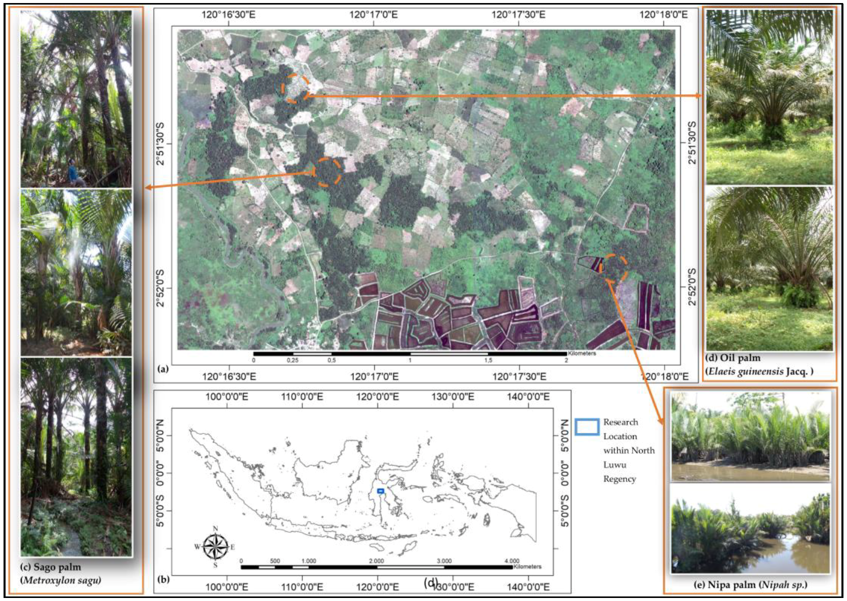
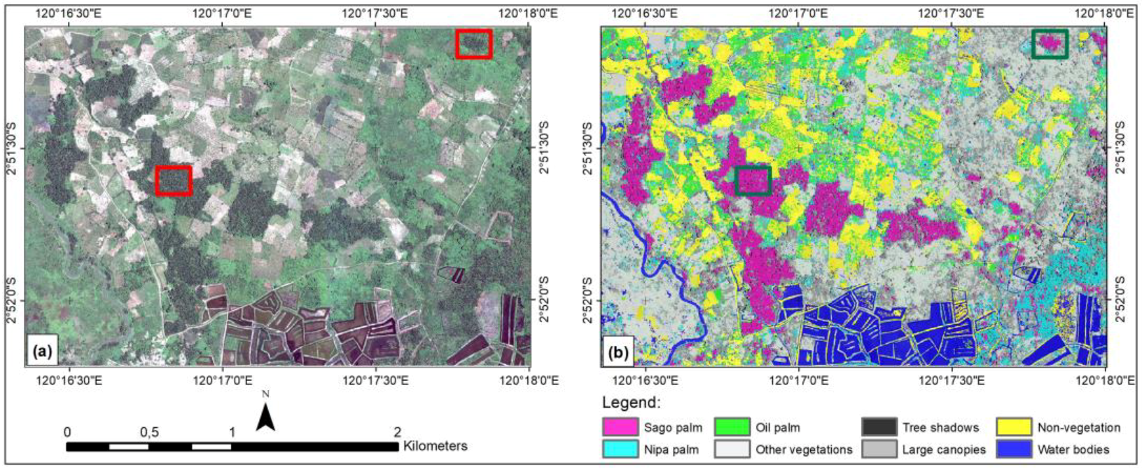
In this study, we used Pleiades-1A imagery of an area around Luwu Raya, which has extensive sago palm coverage (Figure 1). Based on ground truth data and interviews with smallholder farmers, most sago palm trees in Luwu Raya occur in natural or semi-cultivated stands, scattered either in large or small clumps, and with irregular spatial patterns in terms of size, age, and height. Therefore, recognizing sago palm from satellite imagery is very challenging.
According to the context and constraints provided in the studies referenced above, this research was based on the following hypotheses. (i) Image objects of sago palms have specific arithmetic, geometric, and textural features. Through the OBIA approach, RFE and the SVM classifier can reveal the optimum features for sago palm classification. (ii) The mapping of sago palm trees using high-resolution satellite imagery can achieve a high classification accuracy within the OBIA framework, enriched by arithmetic, geometric, and textural features. In support of these hypotheses, this research sought to reveal the important spectral, arithmetic, geometric, and textural features through RFE feature selection and to measure the accuracy of the SVM classifier and analyze the overall classification performance.
The remainder of this paper is organized as follows. Section 2 explains the materials and methods, and Section 3 provides the results. Section 4 discusses the findings in the context of previous research. The final section presents conclusions and suggests future work related to this research.

2. Materials and Methods

This section describes the satellite imagery used and its characteristics, the research location, and the land use land cover (LULC) characteristics within the study area. Figure 2 shows the study methodology flowchart, which is divided into three major steps: preprocessing and image segmentation, sample mining, and classification and analyses. The first step, preprocessing and image segmentation, includes pansharpening of the Pleiades imagery, determining the test image, and generating image objects through image segmentation. This step produces image objects that represent the targeted LULC classes. The second major step is sample mining of non-mainstream data of the classification scheme. This step can guide the researcher in determining sample adequacy, recognizing data characteristics, and evaluating the classifier learnability of the sample. Classifier application to test images provides an estimate of the results. Through sample mining, we also performed feature selection to rank the importance of candidate features. From this step, we acquired the predicted classification accuracy relative to feature contributions, classification parameters, and ranked features. The third major step is classification and analyses, including training and applying the SVM classifier, performing an accuracy assessment, and conducting statistical tests. We carried out 26 executions for this classification scheme and calculated the confusion matrix for each classified image. The OA of image classification was then tested to evaluate its significance, and to determine the range of the most important features for sago palm classification.

2.1. Data and Study Area

This study used Pleiades-1A imagery acquired on 14 September, 2014. Pleiades-1A imagery has four multispectral bands [35] (blue band 430–550 nm, green band 500–620 nm, red band 600–720 nm, and the near-infrared (NIR) band 740–940 nm) and a panchromatic band with a spectrum of 470–830 nm. We received this data during processing of the standard ortho [36], with the geographic coordinate system, CRS WGS84, and projected in south universal transverse Mercator zone 51. The multispectral and panchromatic data were bundled in a separate file; thus, we performed pansharpening using the PANSHARP algorithm built-in to PCI Geomatics [37]. This approach adopted the UNB PanSharp algorithm [38] that applies least squares to greatly reduce the two major deficiencies of pansharpening: color distortion and operator/dataset dependency [37]. Cheng [39] explained the possibility of performing pansharpening of Pleiades imagery using PCI Geomatics. Due to the huge image size and computational complexity, the test image employed a small subset from the pansharpened image, with the following specifications: 6235 × 4008 pixels, 16 bit, and 0.5-m spatial resolution after pansharpening. LULC at this site is dominated by dry crops, sago palm, nipa palm, oil palm, fish ponds, and other vegetation. The heterogeneous landscape in this region is typical of Indonesia, particularly in areas where the sago palm grows.

2.2. Ground Truthing and Known Land Use Land Cover

Ground truthing was conducted to provide field data regarding sago palm distribution. The geographic coordinates of sago palm locations and other LULC data were recorded using a hand-held global positioning system (GPS) receiver. LULC was divided into eight classes: sago palm, nipa palm, oil palm, other vegetation, large canopies, tree shadows, non-vegetation, and water bodies. The LULC classes based on visual observation of the Pleiades-1A imagery are presented in Table 1. Training points for each class were randomly selected within the study area using well-known class locations. The equal sample size (360 points) used for each class was designed to reduce the statistical bias caused by unequal sample sizes. The yellow plus symbol in Table 1 indicates training points, which were converted into image objects after the segmentation process was completed. To meet the needs of the accuracy assessment, another set of checkpoints (200 per class) was carefully selected manually from the image, avoiding any overlap with the training points to avoid statistical bias.

2.3. Segmentation

The first step of OBIA involves subdividing the entire image into smaller pieces, which serve as building blocks for further analyses. This process, referred to as segmentation, generates a simple object to represent the objects of interest [40]. Multiresolution segmentation (MRS), spectral difference, and image object fusion algorithms were used to develop image objects [17]. The MRS algorithm identifies single-image objects of one pixel and merges them with their neighbors based on relative homogeneity criteria. Meanwhile, the spectral difference algorithm maximizes the spectral differences among heterogeneous image objects. The image object fusion algorithm is used to minimize the current image object surface tension and to merge the current image object with neighboring objects or others within the current image.
In eCognition, three criteria are used to define segmentation: scale, shape, and compactness. The scale parameter value is determined using the estimation of scale parameters (ESP) tool [41]. ESP simulations lead to the first break point of the rate of change in local variance (ROC-LV) around the 20-scale parameter, and this value is used as the scale parameter for first-level segmentation. Meanwhile, the shape and compactness values employed are moderate, 0.3–0.5, to maintain good segmentation of tree clumps and tree stands. Spectral band weight is also important in generating an appropriate image object. Typically, NIR band interactions at the leaf scale include high transmittance and reflectance due to photon scattering within leaf air-cell wall interfaces [42]; therefore, the NIR band is weighted more heavily than the other three visible bands of Pleiades-1A imagery. The final image objects were obtained after four segmentation steps, starting with the generation of basic image objects, then minimizing heterogeneity, maximizing spectral distance, and minimizing surface tension. These four steps reduce the number of image objects by approximately 80%, resulting in simpler final image objects, while still maintaining class representation.

2.4. Input Layers and Features

We tested 26 candidate features including four spectral band features, three arithmetic features, seven geometric features, and 12 textural features. Table 2 lists the 26 image object features used. The arithmetic features are customized for the spectral operation to obtain a specific index useful for distinguishing among classes; we used the NDVI as an important vegetation index for vegetation and non-vegetation classification [18], based on maximum difference (MD) and visible brightness (VB). Several geometrical features were considered important, because the image object of sago palm appears to have specific patterns in its shape, polygon, and skeleton. According to a visual assessment of the sago palm canopy, we hypothesized that the sago palm canopy has unique geometric features. Ma et al. [19] utilized 10 geometric features; we used five of these 10 and added two others (degree of skeleton branching and polygon compactness) deemed uniquely suitable for sago palm classification.
The textural feature described by Haralick [21] is most often used with the OBIA approach [18,19,22,23], and is based on GLCM, which tabulates the frequency with which different combinations of pixel gray levels occur in an image. Another way to measure textural components is to use the gray-level difference vector (GLDV), which is the sum of the diagonals of the GLCM [17]. We calculated the GLCM within the image object domain (segmented image) and involved all four bands of the Pleiades imagery in all directions [17]. We applied eight GLCM- and four GLDV-based textural features as input feature candidates. In total, 26 features were calculated using Trimble-eCognition. Although involving features other than spectral features in each classification will enhance the classification accuracy, it is not efficient in terms of the computation time and resources required for the classification process; therefore, feature selection should include ranking the importance of a feature.

2.5. Feature Selection

Feature selection is an important aspect of machine learning and data mining research [33]. We used the RFE method [19], which is an embedded feature selection algorithm for the SVM classifier. SVM-RFE is a rank feature selection method that utilizes the SVM classifier as a so-called wrapper in the feature selection process [34,43,44]. For rank feature selection, SVM-RFE applies a pruning method that first utilizes all features to train a model, and then attempts to eliminate some features by setting the corresponding coefficients to ‘0’ while maintaining model performance [33]. Following Guyon et al. [43], the procedure for executing RFE is iterative, involving the recursive process of training the classifier, computing the ranking criterion for all features, and removing the feature with the smallest ranking criterion.
The feature selection methods were executed using WEKA data mining software (ver. 3.8.2) [45], which includes the AttributeSelectedClassifier tool consisting of the following: LibSVM as a classifier, SVMAttribEval as an evaluator, and Ranker as a search method [46]. The SVMAttributeEval function evaluates the value of an attribute using an SVM classifier, and subsequently ranks attributes using the square of the weight assigned by the SVM. In this research, attribute selection is faced with a multiclass problem, which is handled by ranking the attributes separately using the one-versus-all method and then “dealing” from the top of each pile to obtain a final ranking [47]. The evaluator determines which method is used to assign a value to each subset of attributes, while the search method determines which style of search is performed [48].

2.6. Machine Learning Algorithm

In this study, we applied an SVM classifier in an attempt to find the optimal hyperplane separating classes, by focusing on training cases placed at the edge of the class descriptors [31]. As recommended by Hsu et al. [49], we considered the linear SVM with nonlinear extensions, using the kernel trick to handle SVM calculations with nonlinear distributions. Researchers interested in the advancement of linear SVM, the kernel trick, and its practical applications should refer to several previous studies [28,46,48,50].
When working with nonlinear problems, it is useful to transform the original vectors by projecting them into a higher dimensional space, using the kernel trick so that they can be linearly separated. In this study, we used the radial basis function (RBF) kernel with cost and gamma parameters, which can be found automatically using a grid search [46,48]. The parameters were determined using WEKA data mining software, which provides the GridSearch tool [45]. We used an equal range of cost and gamma parameters, within the range of 10−3 to 103 and with a step size of 101. If the best pair was located on the border of the grid, we let GridSearch extend the search automatically. The GridSearch tool generated a cost parameter of 1000 and a gamma parameter of 0.1 with normalized samples.

2.7. Accuracy Assessment

An accuracy assessment of a classified image requires a reference, either from ground measurements or from reference data such as a map. In this study, we used another set of checkpoints (200 points for each class) independent of the training points, referred to as independent check points (ICPs). The ICPs were selected manually from the test image, without overlapping the training points. The confusion matrices or error matrices [51,52] contain calculated values for a particular class from the classified image relative to the actual class on the ICP. The producer’s accuracy (PA), user’s accuracy (UA), and OA are then calculated from the confusion matrices of each classification scheme. The OA indicates the accuracy of the classification results.
Because the same set of samples was used with 26 classification schemes, the significance of OA between classification schemes was calculated using the McNemar statistical test instead of a z-test [53,54,55]. The McNemar test can be used to compare the performance of any classifier with respect to customized training size, segmentation size [56], and textural features [57]. This test is based on the standardized normal test statistic (z), and the evaluation is based on the chi-square (χ2) distribution with one degree of freedom [53]. The equation of the chi-square test is as follows:
χ 2 = ( f 01 f 10 ) 2 f 01 + f 10
where f01 and f10 are disagreement terms from cross-tabulation of the confusion matrices. We used the 95% confidence interval to evaluate the significance of OA between classification schemes. Our null hypothesis was that there is no significant difference between OA values in a paired classification scheme. The McNemar test will successfully reject the null hypothesis when the calculated χ2 is greater than 3.84 or its probability (p-value) is less than 0.05, and thus conclude that the two classification schemes have a statistically significant difference.

3. Results

We concentrated on three vegetation classes: sago palm, nipa palm, and oil palm, due to their spectral response similarities.

3.1. Overall Classification Performance

The performance of the SVM classifier varied along with changes in feature ranking. Figure 3 shows the feature ranking performance for both training samples (blue line) and ICPs (brown line). Based on 360 samples from each class, the SVM classifier successfully estimated the correctly classified instances (CCIs) [46] and reached a peak at the 10 most important features (marked by a red circle on the blue line in Figure 3, with a CCI of 85.55%); however, the CCI values appeared to be saturated thereafter. When the classifier arrived at the 24 most important features and beyond, CCI values tended to decrease, as the model appeared to become overwhelmed with the number of features involved.
A similar result was obtained when the accuracy of the classified images was tested using the ICP; the OA values (brown line in Figure 3) were similar to CCI values until reaching a peak at the eight most important features (marked by a black circle on the brown line in Figure 3, with an OA of 85.00%). From the ninth most important feature upwards, OA tended to decrease until reaching its lowest value at the 20th most important feature (marked by a green circle on the brown line in Figure 3; OA of 79.72%), and only insignificantly small fluctuations occurred thereafter. From the most important to the eighth most important feature, the model seemed to fit normally, but became overfitted thereafter for lower ranking features. Overfitting is a common problem in machine learning, in which a model performs well on training samples but does not generalize well for test images [58]. Our model faced the same problem when used on training samples and test images, where too many features led to very complex computations and resulted in a lower classification accuracy. Our model’s “sweet spot” [59] was at eight features, where it showed an optimal performance in both training and test images.

3.2. Feature Selection

The important features were ranked using the SVM-RFE method. The blue line in Figure 3 shows the change in CCI with increasing feature ranking number; we can infer that after the inclusion of the first 10 features (marked by a red circle), the CCI values appeared to be in a steady state and almost no subsequent changes occurred. The first 10 most important features included the following: three spectral features, three arithmetic features, three textural features, and one geometric feature. The spectral features are important in this study for classifying imagery into eight classes; however, the degree of importance of the NIR band is reduced with NDVI, MD, and VB. The first two major features contain spectral information, i.e., the red and blue bands. The next two most important features are textural features, namely, GLDV contrast and GLCM correlation; this made it evident that to improve the classification accuracy and obtain better separation among classes, textural features must be considered. The other four features in the top 10 included three arithmetic features and one geometric feature (the degree of skeleton branching).

3.3. Image Segmentation

Figure 4 shows the results of segmentation, i.e., the image objects. The first level of image objects generated from the MRS algorithm tended to be over-segmented and massive (panel b), which was intentional to allow single-tree objects to be identified. Segmentation shape values of 0.1 and 0.3 can produce accurate boundaries for image objects [60]; we chose a moderate shape value of 0.3. To maintain the level of detail to identify sago palm clumps (indicated by green circles in the figure), we used a 20-scale parameter at the first segmentation level. The next segmentation process was designed to optimize the image object in terms of representing the actual object in the field. After executing the second and third MRS algorithms (panels c and d), small objects such as single trees could be separated clearly (white circles in panels a and d). Although the size of the image object appeared very small, the training samples were generated homogeneously and were able to accommodate finer class limits during refinement of the classification results.
Panel (e) shows the fourth segmentation level, which applied a spectral difference algorithm to maximize the spectral difference and to merge neighboring objects according to their mean layer intensities. That image was also processed with the image object fusion algorithm to optimize the final image objects. As seen in panels (d) and (e), small image objects merged into surrounding dominant image objects (indicated by blue circles). The image object fusion algorithm is useful for mapping single-tree objects, such as individual oil palm trees (white circles in panel f), while merging unnecessary image objects. A good performance was also observed for dense sago palm clumps and large canopies, which were classified correctly (green and red circles in panel f, respectively). The final segmentation level left about 20% of the total image objects, and this final image object maintained a level of detail for sago palm of either clumps or single trees.
Measures for segmentation accuracy relative to a set of reference data are needed [61], because the segmented image will determine the classification results. The overall segmentation accuracy can assist researchers in objective selection and determination of segmentation parameters. Segmentation accuracy assessments have been widely published. Zhang [62] introduced two families of an evaluation method for image segmentation, i.e., empirical goodness and discrepancy methods. Clinton et al. [61] provided a comprehensive review of segmentation goodness measurement methods, and Bao et al. [63] demonstrated Euclidean distance and segmentation error index measures. All of these measurement approaches show the need for reference data to measure segmentation accuracy. Reference data are commonly in a vector format, such as a polygon. Therefore, the provision of vector-based reference data needs to be considered for justification of the segmentation results.

3.4. Feature Performance

We classified all feature rankings consecutively, starting with the inclusion of 26 features until only one feature remained; thus, within the so-called classification scheme, there are 26 classification schemes in total. The OA of each classification scheme is shown in Figure 3 (brown line). For example, the classification schemes involving only one feature (the red band) and two features (the red and blue bands) resulted in the lowest accuracies (50.86% and 62.09%, respectively), which were nonetheless higher than the accuracy predicted from the training samples (48.04% and 58.99%, respectively; blue line in Figure 3). The classified image accuracy continued to increase until the number of features reached eight (resulting in the highest OA of 85.00%), and then did not rise further as the number of features gradually increased to 26.
Table 3, Table 4 and Table 5 show the confusion matrices from the three classification schemes, i.e., with eight, 10, and 26 features, respectively, which are important due to their feature contribution to classification accuracy. The confusion between sago palm and other vegetation classes (nipa palm, oil palm, other vegetation, and large canopies) occurred in all classification schemes, and is understandable because these five classes have overlapping spectral responses and similar geometric properties. There is significant confusion between oil palm and sago palm in every classification scheme, and it should be noted that in this study, oil palm trees were in the rosette stage. At the highest OA (eight most important features), the PA and UA of sago palm also held the highest values compared with other classification schemes.
Associations in OA between classification schemes were tested using the McNemar test to determine statistical significance. Table 6 shows a simple cross-tabulation (sometimes called a contingency table) summarizing the classified and actual classes of a selected classification scheme pair, i.e., eight versus 10 features. The table is a type of 2 × 2 matrix containing binary data for correct and incorrect classifications [53], and it was derived from the original table from which the confusion matrices were generated.
From Table 6, let f00 = 171, f01 = 53, f10 = 74, and f11 = 1216; then, cross-tabulation includes 127 samples (53 + 74) with disagreement between the eight- and 10-feature SVM classifiers. The main diagonal elements (f00 and f11) in Table 6 and Table 7 do not contribute to making a statistical decision, because the marginal homogeneity in the 2 × 2 matrices is equivalent to f00 = f10 [54]. The McNemar test focused solely on f01 and f10, the disagreement elements, to determine whether eight features are better than 10 features. Chi-square was calculated using Equation (1). Based on the disagreement component in Table 6, we obtained a chi-square of 3.15, which corresponds to a p-value of 0.0759. This p-value is greater than 0.05; therefore, the null hypothesis should be retained, stating that the classification did not significantly differ between eight and 10 features. Accordingly, either one can be used. In contrast, the results of analyses using the data shown in Table 7 had a chi-square of 16.08, which corresponds to a p-value of 0.0001. This is smaller than 0.05, thus rejecting the null hypothesis; additionally, these results indicate that the SVM classifier has a better OA with eight features than with 26 features.
Other McNemar test results are shown in Table 8; for example, classification pair #1 and #2 had a statistically significant difference, and so did classification pairs #6 and #7. Because SVM classifiers with 15 features or more tended to decrease (brown line in Figure 3), the McNemar test obtained a significant difference with regards to their OA compared with using eight features. On the other hand, the classification pair #3 and #5 did not show a statistically significant difference, which means that within the range of the 7th–14th most important features, the SVM classifier will generate a higher classification accuracy.

3.5. Classified Image

Figure 5 depicts the full extent of the test image (left image) and the classified image from the highest OA (right image), which uses eight features. Visually, the classified image looks relatively satisfactory for the sago palm class. Panel (a) shows Pleiades-1A imagery, and the red boxes represent sago palm clumps and single trees. Panel (b) depicts the classified image, where the sago palm class is shown in magenta (green box). Post-classification enhancement will reduce or eliminate the salt-and-pepper effect on the classified image. However, in this study, post-classification improvement was not conducted, as we wanted to observe the original performance of the algorithm and the classification scheme.
We conducted SVM classification by only involving the original four spectral bands as a starting reference, regardless of whether additional features would improve the OA. Figure 6 (panels a and c) shows the classified images; at a glance, visual assessment appears satisfactory in that there is no significant difference between panels a and b. However, with more thorough tracing, the misclassifications were more clearly resolved. The green box in panel (c) shows misclassification between the sago palm and nipa palm, either at the edge of the sago palm class or in the middle of the sago palm clump. Without post-classification refinement, this four spectral band-classification result will greatly reduce the actual coverage of the sago palm stand. In contrast, the green box in panel (d) shows less misclassification between the sago and nipa palms. The OA of the four spectral band classification only reached 83%, compared with 85% after including other features, i.e., textural, arithmetical, and geometrical features. The PA of the sago palm class of the four-band classification was also lower than that including other features (80% vs. 88% respectively).
Figure 7 compares Pleiades-1A imagery with the classified images using eight, 20, and 26 features. The OA also showed visual improvement in classified images. Among the three classified images in Figure 7, panel (b) had the highest OA and showed better classification results according to visual assessment. The black boxes indicate misclassified image objects of sago palm, nipa palm, and water bodies. Most of the misclassified water bodies are actually tree shadows. In panel (b), the SVM classifier with eight features resulted in a more homogenous and generalized classified image, especially for the sago palm class. Classes other than those three had relatively few misclassifications; the oil palm class had consistent classification, even for a single tree (red box). The oil palm class exhibited some misclassification with other classes (panels c and d). As shown in panel (c), 20 features, with an OA of 79.72%, retained misclassified small water bodies and nipa palm objects. Likewise, 26 features gave an OA of 80.91%, but most small objects such as water bodies and nipa palm were misclassified (panel d), as they should have been classified as sago palm. As true for all classes, using eight features gave the highest PA (88.00%) and UA (81.48%) values for the sago palm class, and this class was displayed most uniformly.

4. Discussion

Previous research on sago palm mapping, as described in the Introduction section, has employed the MLC as the classifier to stack and analyze multi-source datasets. Our research applied the SVM as a learning algorithm, which is a promising machine learning methodology [28] that has recently been used for a wide range of applications in remote sensing. We utilized high-resolution full-band satellite imagery from Pleiades-1A. The red band is the most important, exhibiting the strongest absorption in the majority of tree species due to the presence of chlorophyll, used for photosynthesis [23]. The dominant chlorophyll pigments account for almost all absorption in the red and blue bands, and carotenoid pigments extend this absorption into the blue-green bands [64]. Meanwhile, reflectance of the NIR band at the leaf level is controlled by water content, due to chemically driven absorption [12], because most chlorophyll pigments do not significantly absorb infrared light [64]. When the amount of water increases, the transmittance of the NIR band will be enhanced [23], particularly at wavelengths longer than about 1100 nm, which water strongly absorbs [64]. In this context, the importance of selecting particular spectral features for certain vegetation classes is evident, because the spectral response depends on their chemical and structural characteristics [64]. According to in situ spectral measurements [10], from 870 nm upward, oil palm is separable from nipa palm and sago palm, and evidence shows that sago palm is separable from nipa palm around 935–1010 nm. Unfortunately, the Pleiades-1A does not have a spectral band at 935–1010 nm; therefore, we added other features to improve the classification accuracy, including arithmetical, geometrical, and textural features.
This research site contained several vegetation classes; accordingly, we added the vegetation index NDVI, which is useful for distinguishing among green vegetation classes [18] and also between vegetation and non-vegetation. Other important arithmetic features, MD [19] and VB, were considered due to their high contrast between sago palm and nipa palm. Visual assessment of a natural-color composite of Pleiades-1A imagery found textural differences between sago palm and nipa palm in clumps; thus, the inclusion of textural features was expected to make a strong contribution to the classification accuracy. The 12 textural features used by Haralick [21] were selected as input candidates [19]. Object-based image analyses require a segmented image as an input for classification, with every class represented by many image objects depending on the scale, shape, and compactness parameters used during the segmentation process. Every image object has certain geometric characteristics; hence, we included the seven geometric features listed in Table 2, of which five were used by Ma et al. [19].
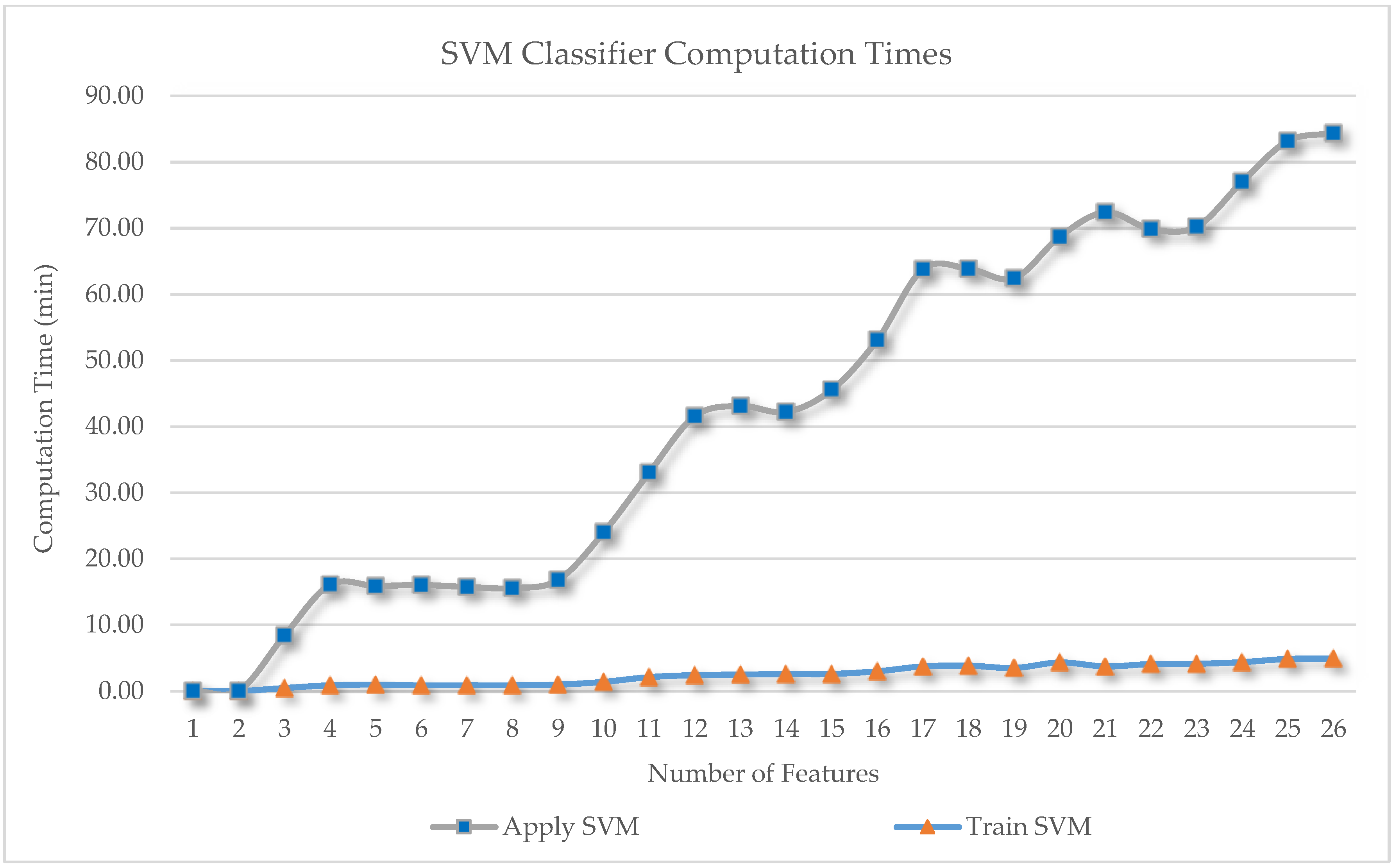
Involving more feature space in the classification scheme has great potential for improving the accuracy, but our data dimensionality became very high. We can estimate computational complexity by multiplying the 26 features by eight classes, with 360 samples for each class and 161,168 image objects at the final segmentation level; therefore, we applied feature selection to reduce data dimensionality and computational complexity. Based on our computer performance (processor: Intel (R) Core (TM) i7-3770 CPU @ 3.40 GHz (eight CPUs); memory: 32,768 MB RAM), we recorded the computation time for these 26 classification schemes. From the results displayed in Figure 8, the amount of computation time required increased in an almost linear manner as a function of the number of features involved in the classification. The computation time of the training SVM classifier (the orange triangle in Figure 8) is always shorter than that when applying an SVM classifier (the blue square in Figure 8), because it is only applied to the sample. The difference in time required between one feature and 26 features was significant, at ~80 min, considering that our test image size was relatively small (195 MB). At the highest OA, with eight features, the computation time was ~15 min, which is very fast compared with that required for 26 features. If the test image size increased to the gigabyte range, we would expect the computation time to be considerable. Therefore, if the research project covers a wide area and uses very high-resolution satellite imagery, performing feature selection prior to classification is recommended. Our research goal was to obtain the highest possible classification accuracy; thus, we used a feature-important evaluation method [19], i.e., SVM-RFE, with our SVM learning method. According to experimental analyses by Cai et al. [34], SVM-RFE provides the best accuracy, of nearly 100%, outperforming other feature-selection methods. We executed SVM-RFE with known sample classes and obtained the 10 most important features, with a CCI of 85.55%. This predicted classification accuracy is still considered high due to the presence of other similar tree species in the study area, i.e., nipa palm and oil palm.
Our sample mining showed that three visible spectral bands remained important (blue, green, and red bands); thus, the NIR band was eliminated and replaced with the three arithmetic features (NDVI, MD, and VB). One geometric feature, the degree of skeleton branching, was also included among the 10 most important features, because image objects of the sago palm class appear to have a high degree of skeleton branching. Within the 10 most important features, textural features play an important role, as do spectral features, i.e., GLDV contrast, GLCM correlation, and GLCM angular second moment, which contributed about 30% to the model. For crop identification, Peña-Barragán et al. [18] found that the textural features discussed by Haralick [21] contributed 6–14% to the OBIA approach with a decision tree algorithm. The difference in the contribution of textural features could be due to the use of different algorithms and target classes. Ghosh and Joshi [23] noted that GLCM mean is more useful than other GLCM textural features for mapping bamboo patches in the lower Gangetic plains of the state of West Bengal, India, using WorldView-2 imagery. Based on the discussion above, we can presume that the role and type of textural features depend on the classifier algorithm, feature selection method, target class, image sensor, and image scene.
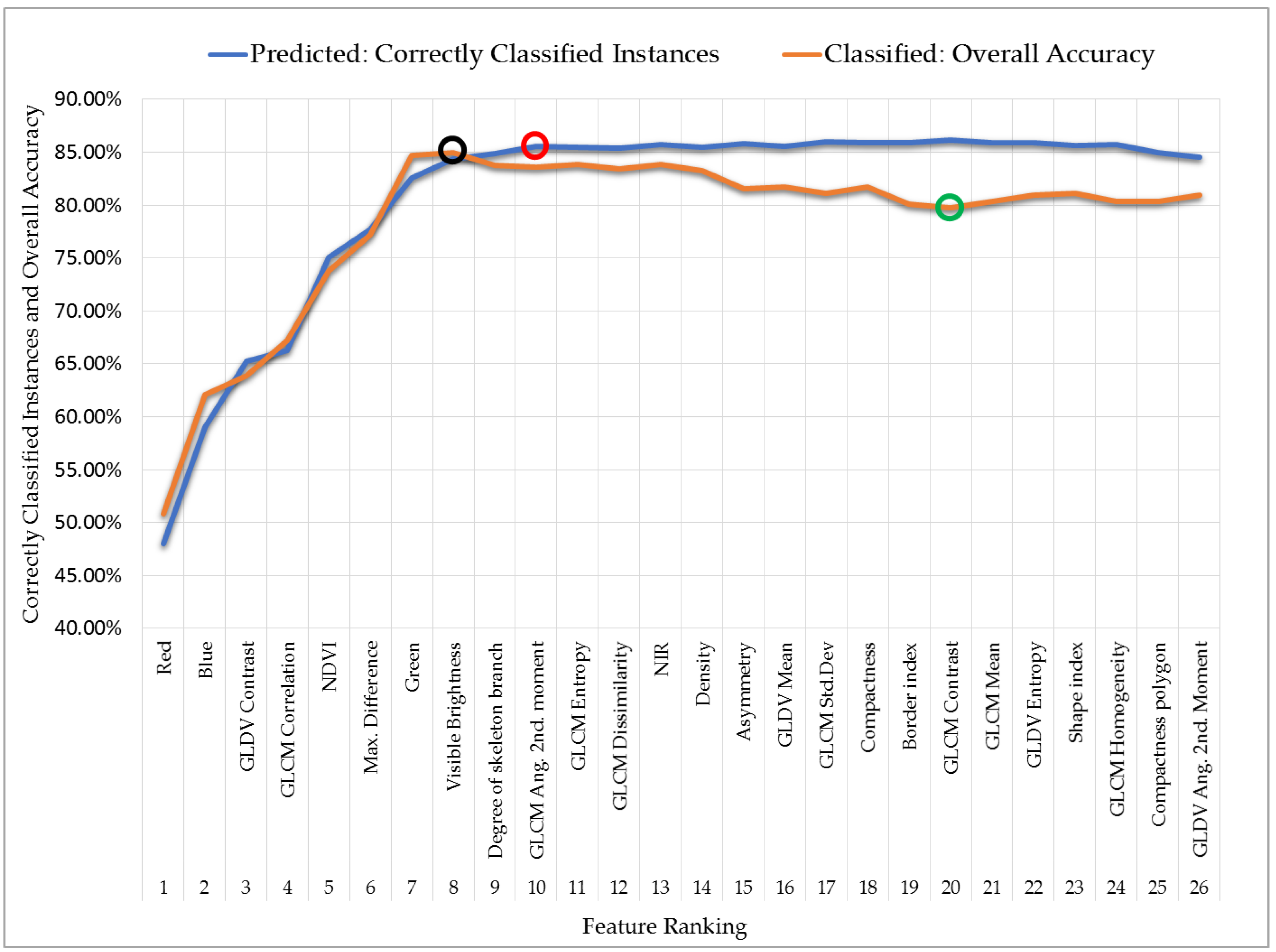
When the ranked features were applied to the test image, the results showed normal fitting for the eight most important features, achieving the highest OA of 85.00% (with a PA and UA for sago palm of 88.00% and 81.48%, respectively); thereafter, the data appeared to be overfitted (brown line in Figure 3). The degree of skeleton branching and the GLCM angular second moment contribute less to the model; when these two features (the 9th and 10th most important features) were involved in the classification, the model was overfitted. Meanwhile, the textural features of the GLCM correlation and GLDV contrast remained important, improving the OA from 62% to 67% (for details, see Figure 3). According to the sample scatter plot, most GLDV contrast values of the nipa palm class were higher than those of the sago palm class; thus, these values are useful to distinguish these classes. In a harsh critique of thematic map accuracy derived from remote sensing [65], an OA of 85% was still considered acceptable; researchers interested in the historical origin of this value should access the original study [66]. Additionally, Foody et al. [65] and Congalton et al. [67] provide in-depth discussions of image classification accuracy assessment.
Regarding the accuracy of our classified image, the highest OA of 85% may still be improved by applying random sampling, as described in several studies [67,68] and recommended by Ma et al. [69]. Even though we used another set of checkpoints independent of the training points, some subjectivity may have been introduced into the OA due to the manual selection approach. In our opinion, an OA of 85% is still relatively high compared with other research findings on palm-tree classification. Previous studies on sago palm mapping have mostly utilized medium-resolution satellite imagery, such as Santillan [8] and Santillan et al. [7]. When they only used spectral information from ALOS AVNIR 2 or LANDSAT ET+, the UA and PA of sago palm classification reached 77% and 82%, respectively; in contrast, a UA of sago palm classification achieved 91.37% when several medium-resolution satellite images were combined. Other palm-tree classifications, such as coconut tree [70] and babassu palm (Attalea speciosa) [11], also resulted in a lower classification accuracy, that is, an OA value of 76.67% for coconut tree and 75.45% for babassu palm. Li et al. [71] achieved better classification results when performing oil palm plantation mappings in Cameroon using PALSAR 50 m; OA ranging from 86% to 92% was accomplished using an SVM classifier. To evaluate the significance of OA values obtained from our own research, we conducted a McNemar statistical test.
McNemar tests indicated that using seven to 14 of the most important features was optimal. Research is most effective when using as few features as possible while still obtaining a high accuracy. Generally, the optimal number of important features is small. For example, Cai et al. [34] used 10 and 15 features with SVM-RFE to achieve nearly 100% accuracy. Ma et al. [19] reported using 10–20 features for the SVM classifier. Our method requires seven to 14 features for sago palm classification; the results are comparable to those of previous studies within an OBIA framework with an SVM classifier. Differences in the optimum numbers of features should be considered in image classification depending on the heterogeneity of test images. The development of other important features to obtain a classification accuracy higher than 85% in sago palm classification remains very challenging.

5. Conclusions

Sago palm classification using the OBIA approach and SVM classifier should consider other features in addition to the original spectral bands from satellite imagery. The OA of four-band classification can only reach 83%; the addition of textural, arithmetical, and geometrical features increases the OA to 85%. The PA of sago palm was also lower than that including other features (80% vs. 88%, respectively). Including the additional features in the classification increases the amount of data to be processed; thus, the computation time and resources required increase as well. As such, the feature selection algorithm is highly recommended.
This study reconfirms the importance of feature selection prior to the classification process. Our major finding is the revelation of the most important features for sago palm classification within an OBIA framework. We used SVM-RFE to assess the importance of the role of each feature, generating a ranking of features. The SVM classifier learned from the training samples and, when applied to the test image, produced normal fitting based on up to eight of the most important features, which resulted in the highest OA of 85.00%. For sago palm classification, it is important to include textural and arithmetic features such as GLDV contrast, GLCM correlation, NDVI, MD, and VB, in addition to spectral information. In this study, the McNemar test was used to evaluate associations among OA values of classification schemes, and the optimum range of ranked features was identified.
Generally speaking, the palm-tree classification is very challenging, especially for sago palm classification in our study area. The sago palm trees in Luwu Raya are are generally natural or semi-cultivated, and tend to be scattered either in large or small clumps with irregular spatial patterns in size, age, and height. Coupled with the presence of other similar palm-tree species that have similar spectral responses and textures, such as nipa palm and oil palm, this complicates the identification process. Thus, a specific sago palm classification scheme is required to better understand its spatial and spectral characteristics. The OA value of 85% can certainly be improved through further revisions of our sampling approach for accuracy assessment, measurement of segmentation accuracy, atmospheric correction, and geometric correction when using multi-strip images.

Author Contributions

S.H. designed the experiments, performed the experiments, analyzed data, and wrote the paper; M.M. conceived and designed the experiments, contributed methods and analysis tools, advised on research progress, and edited the paper; S.B. and D.A.R. suggested the line of research, and advised on research progress and paper contents.

Funding

This research received no external funding.

Acknowledgments

The Pleiades-1A data were provided by LAPAN Remote Sensing Technology and Data Center under MoU with AIRBUS Defence and Space.

Conflicts of Interest

The authors declare no conflict of interest.

References

  1. Konuma, H. Status and Outlook of Global Food Security and the Role of Underutilized Food Resources: Sago Palm. In Sago Palm: Multiple Contributions to Food Security and Sustainable Livelihoods; Ehara, H., Toyoda, Y., Johnson, D.V., Eds.; Springer: Singapore, 2018; pp. 3–16. ISBN 978-981-10-5269-9. [Google Scholar] [Green Version]
  2. Flach, M. Sago palm. Metroxylon sagu rottb. Promoting the Conservation and Use of Underutilized and Neglected Crops; Heller, J., Engels, J., Hammer, K., Eds.; IPGRI: Rome, Italy, 1997; ISBN 92-9043-314-X. [Google Scholar]
  3. Karim, A.A.; Tie, A.P.-L.; Manan, D.M.A.; Zaidul, I.S.M. Starch from the Sago (Metroxylon sagu) Palm Tree Properties, Prospects, and Challenges as a New Industrial Source for Food and Other Uses. Compr. Rev. Food Sci. Food Saf. 2008, 7, 215–228. [Google Scholar] [CrossRef] [Green Version]
  4. Mcclatchey, W.; Manner, H.I.; Elevitch, C.R. Metroxylon amicarum, M. paulcoxii, M. sagu, M. salomonense, M. vitiense, and M. warburgii (sago palm) ver. 2.1. In Species Profiles for Pacific Island Agroforestry; Elevitch, C.R., Ed.; Permanent Agriculture Resources (PAR): Hōlualoa, HI, USA, 2006; pp. 1–23. Available online: http://agroforestry.org/free-publications/traditional-tree-profiles (accessed on 16 February 2018).
  5. Abbas, B. Genetic diversity of sago palm in Indonesia based on chloroplast DNA (cpDNA) markers. Biodivers. J. Biol. Divers. 2010, 11, 112–117. [Google Scholar] [CrossRef]
  6. Bintoro, M.H.; Iqbal Nurulhaq, M.; Pratama, A.J.; Ahmad, F.; Ayulia, L. Growing Area of Sago Palm and Its Environment. In Sago Palm: Multiple Contributions to Food Security and Sustainable Livelihoods; Ehara, H., Toyoda, Y., Johnson, D.V., Eds.; Springer: Singapore, 2018; pp. 17–29. ISBN 9789811052699. [Google Scholar] [Green Version]
  7. Santillan, J.R.; Santillan, M.M.; Francisco, R. Using remote sensing to map the distribution of sago palms in Northeastern Mindanao, Philippines: Results based on landsat ETM+ image analysis. In Proceedings of the 33rd Asian Conference on Remote Sensing—Aiming Smart Space Sensing, Pattaya, Thailand, 26–30 November 2012. [Google Scholar]
  8. Santillan, J.R. Mapping the starch-rich sago palsm through Maximum likelihood classification of multi-source data. In Proceedings of the 2nd Philippine Geomatics Symposium (PhilGEOS): Geomatics for a Resilient Agriculture and Forestry, University of The Philippines, Diliman, Quezon City, Philippines, 28–29 November 2013; pp. 1–9. [Google Scholar]
  9. Jojene, R. Santillan & Meriam Makinano-Santillan Recent Distribution of Sago Palms in the Philippines. In BANWA Monograph Series 1 Mapping Sago: Anthropological, Biophysical and Economic Aspects; Paluga, M.J.D., Ed.; University of the Philippines: Mindanao, Philippines, 2016; p. 186. ISBN1 6219560701. ISBN2 9786219560702. [Google Scholar]
  10. Santillan, M.M.; Japitana, M.V.; Apdohan, A.G.; Amora, A.M. Discrimination of Sago Palm from Other Palm Species Based on in-Situ Spectral Response Measurements. In Proceedings of the 33rd Asian Conference on Remote Sensing—Aiming Smart Space Sensing, Ambasador City Jomtien Hotel, Pattaya, Thailand, 26–30 November 2012. [Google Scholar]
  11. Dos Santos, A.M.; Mitja, D.; Delaître, E.; Demagistri, L.; de Souza Miranda, I.; Libourel, T.; Petit, M. Estimating babassu palm density using automatic palm tree detection with very high spatial resolution satellite images. J. Environ. Manag. 2017, 193, 40–51. [Google Scholar] [CrossRef] [PubMed] [Green Version]
  12. Fassnacht, F.E.; Latifi, H.; Stereńczak, K.; Modzelewska, A.; Lefsky, M.; Waser, L.T.; Straub, C.; Ghosh, A. Review of studies on tree species classification from remotely sensed data. Remote Sens. Environ. 2016, 186, 64–87. [Google Scholar] [CrossRef]
  13. Chemura, A.; van Duren, I.; van Leeuwen, L.M. Determination of the age of oil palm from crown projection area detected from WorldView-2 multispectral remote sensing data: The case of Ejisu-Juaben district, Ghana. ISPRS J. Photogramm. Remote Sens. 2015, 100, 118–127. [Google Scholar] [CrossRef]
  14. Puissant, A.; Rougier, S.; Stumpf, A. Object-oriented mapping of urban trees using Random Forest classifiers. Int. J. Appl. Earth Obs. Geoinf. 2014, 26, 235–245. [Google Scholar] [CrossRef]
  15. Wang, D.; Wan, B.; Qiu, P.; Su, Y.; Guo, Q.; Wu, X. Artificial Mangrove Species Mapping Using Pléiades-1: An Evaluation of Pixel-Based and Object-Based Classifications with Selected Machine Learning Algorithms. Remote Sens. 2018, 10, 294. [Google Scholar] [CrossRef]
  16. Blaschke, T. Object-based image analysis for remote sensing. ISPRS J. Photogramm. Remote Sens. 2010, 65, 2–16. [Google Scholar] [CrossRef]
  17. Gmbh, T.G. Trimble eCognition Developer 9.0 User Guide; ISBN in Part on Third-Party Software Components: eCognition Developer © 2014 Trimble Germany GmbH; Trimble Germany GmbH: Munich, Germany, 2014. [Google Scholar]
  18. Peña-Barragán, J.M.; Ngugi, M.K.; Plant, R.E.; Six, J. Object-based crop identification using multiple vegetation indices, textural features and crop phenology. Remote Sens. Environ. 2011, 115, 1301–1316. [Google Scholar] [CrossRef] [Green Version]
  19. Ma, L.; Fu, T.; Blaschke, T.; Li, M.; Tiede, D.; Zhou, Z.; Ma, X.; Chen, D. Evaluation of Feature Selection Methods for Object-Based Land Cover Mapping of Unmanned Aerial Vehicle Imagery Using Random Forest and Support Vector Machine Classifiers. ISPRS Int. J. Geo-Inf. 2017, 6, 51. [Google Scholar] [CrossRef]
  20. Zhang, X.; Cui, J.; Wang, W.; Lin, C. A Study for Texture Feature Extraction of High-Resolution Satellite Images Based on a Direction Measure and Gray Level Co-Occurrence Matrix Fusion Algorithm. Sensor 2017, 17, 147. [Google Scholar] [CrossRef] [PubMed]
  21. Haralick, R.M.; Shanmugam, K.; Dinstein, I. Textural Features for Image Classification. IEEE Trans. Syst. Man Cybern. 1973, SMC-3, 610–621. [Google Scholar] [CrossRef]
  22. Zylshal; Sulma, S.; Yulianto, F.; Nugroho, J.T.; Sofan, P. A support vector machine object-based image analysis approach on urban green space extraction using Pleiades-1A imagery. Model. Earth Syst. Environ. 2016, 2, 54. [Google Scholar] [CrossRef]
  23. Ghosh, A.; Joshi, P.K. A comparison of selected classification algorithms for mapping bamboo patches in lower Gangetic plains using very high-resolution WorldView 2 imagery. Int. J. Appl. Earth Obs. Geoinf. 2014, 26, 298–311. [Google Scholar] [CrossRef]
  24. Franklin, S.E.; Hall, R.J.; Moskal, L.M.; Maudie, A.J.; Lavigne, M.B. Incorporating texture into classification of forest species composition from airbone multispectral images. Int. J. Remote Sens. 2000, 21, 61–79. [Google Scholar] [CrossRef]
  25. Bonaccorso, G. Machine Learning Algorithms: A Reference Guide to Popular Algorithms for Data Science and Machine Learning; Phadkay, V., Singh, A., Eds.; Fisrt Publ.; Packt Publishing Ltd.: Birmingham, UK, 2017; ISBN 978-1-78588-962-2. [Google Scholar]
  26. Burges, C.J.C. A Tutorial on Support Vector Machines for Pattern Recognition. Data Min. Knowl. Discov. 1998, 2, 121–167. [Google Scholar] [CrossRef]
  27. Cubillas, J.E.; Japitana, M. The application of support vector machine (SVM) using cielab color model, color intensity and color constancy as features for ortho image classification of Benthic Habitats in Hinatuan, Surigao del sur, Philippines. Int. Arch. Photogramm. Remote Sens. Spat. Inf. Sci. 2016, 41, 189–194. [Google Scholar] [CrossRef]
  28. Mountrakis, G.; Im, J.; Ogole, C. Support vector machines in remote sensing: A review. ISPRS J. Photogramm. Remote Sens. 2011, 66, 247–259. [Google Scholar] [CrossRef]
  29. Immitzer, M.; Atzberger, C.; Koukal, T. Tree Species Classification with Random Forest Using Very High Spatial Resolution 8-Band WorldView-2 Satellite Data. Remote Sens. 2012, 4, 2661–2693. [Google Scholar] [CrossRef] [Green Version]
  30. Åkerblom, M.; Raumonen, P.; Mäkipää, R.; Kaasalainen, M. Automatic tree species recognition with quantitative structure models. Remote Sens. Environ. 2017, 191, 1–12. [Google Scholar] [CrossRef]
  31. Tzotsos, A. A Support Vector Machine Approach for Object Based Image Analysis. In Proceedings of 1st International Conference on Object-Based Image Analysis (OBIA 2006); Stefan, L., Thomas Blaschke, E.S., Eds.; Salzburg University: Salzburg, Austria; Volume XXXVI-4/C4.
  32. Qian, Y.; Zhou, W.; Yan, J.; Li, W.; Han, L. Comparing machine learning classifiers for object-based land cover classification using very high resolution imagery. Remote Sens. 2015, 7, 153–168. [Google Scholar] [CrossRef]
  33. Tang, J.; Alelyani, S.; Liu, H. Feature Selection for Classification: A Review. In Data Classification: Algorithms and Applications; Aggarwal, C.C., Ed.; Chapman and Hall/CRC Press: London, UK, 2014; pp. 37–64. ISBN 978-1-4665-8674-1. [Google Scholar]
  34. Cai, J.; Luo, J.; Wang, S.; Yang, S. Feature selection in machine learning: A new perspective. Neurocomputing 2018, 70–79. [Google Scholar] [CrossRef]
  35. Airbus Defence and Space Geo-Intelligence Pléiades Spot the Detail. Available online: http://www.intelligence-airbusds.com/files/pmedia/public/r61_9_geo_011_pleiades_en_low.pdf (accessed on 3 June 2018).
  36. ASTRIUM an EADS Company. Pléiades Imagery User Guide; Coeurdevey, L., Gabriel-Robez, C., Eds.; v 2.0.; ISBN in Part on Third-Party Software Components: Pléiades Direct Receiving Station; Astrium GEO-Information Services: Toulouse, France, 2012. [Google Scholar]
  37. Geomatics, P. PANSHARP. Available online: http://www.pcigeomatics.com/geomatica-help/references/pciFunction_r/modeler/M_pansharp.html (accessed on 2 July 2018).
  38. Zhang, Y.; Mishra, R.K. From UNB PanSharp to Fuze Go—The success behind the pan-sharpening algorithm. Int. J. Image Data Fusion 2014, 5, 39–53. [Google Scholar] [CrossRef]
  39. Cheng, P. Geometric Correction, Pan-sharpening and DTM Extraction: Pleiades Satellite. Available online: http://www.pcigeomatics.com/pdf/Geomatica-Pleiades-Processing.pdf (accessed on 25 July 2018).
  40. Benz, U.C.; Hofmann, P.; Willhauck, G.; Lingenfelder, I.; Heynen, M. Multi-resolution, object-oriented fuzzy analysis of remote sensing data for GIS-ready information. ISPRS J. Photogramm. Remote Sens. 2004, 58, 239–258. [Google Scholar] [CrossRef] [Green Version]
  41. Drǎguţ, L.; Tiede, D.; Levick, S.R. ESP: A tool to estimate scale parameter for multiresolution image segmentation of remotely sensed data. Int. J. Geogr. Inf. Sci. 2010, 24, 859–871. [Google Scholar] [CrossRef]
  42. Clark, M.L.; Roberts, D.A.; Clark, D.B. Hyperspectral discrimination of tropical rain forest tree species at leaf to crown scales. Remote Sens. Environ. 2005, 96, 375–398. [Google Scholar] [CrossRef]
  43. Guyon, I.; Weston, J.; Barnhill, S.; Vapnik, V. Gene Selection for Cancer Classification using Support Vector Machines. Mach. Learn. 2002, 46, 389–422. [Google Scholar] [CrossRef] [Green Version]
  44. Kohavi, R.; John, G.H. Wrappers for feature subset selection. Artif. Intell. 1997, 97, 273–324. [Google Scholar] [CrossRef]
  45. Hall, M.; Frank, E.; Holmes, G.; Pfahringer, B.; Reutemann, P.; Witten, I.H. The WEKA data mining software. ACM SIGKDD Explor. Newsl. 2009, 11, 10. [Google Scholar] [CrossRef]
  46. Witten, I.H.; Frank, E. Data Mining: Practical Machine Learning Tools and Techniques, 2nd ed.; Morgan Kaufmann Publishers is an Imprint of Elsevier: San Francisco, CA, USA, 2005; ISBN 0-12-088407-0. [Google Scholar]
  47. Frank, E.; Hall, M.; Holland, K. SVMAttributeEval3. Available online: http://weka.sourceforge.net/doc.packages/SVMAttributeEval/weka/attributeSelection/SVMAttributeEval.html (accessed on 5 November 2018).
  48. Bouckaert, R.R.; Frank, E.; Hall, M.; Kirkby, R.; Reutemann, P.; Seewald, A.; Scuse, D. WEKA Manual for Version 3-8-2; The University of Waikato: Hamilton, New Zealand, 2017; Available online: http://sourceforge.mirrorservice.org/w/we/weka/documentation/3.8.x/WekaManual-3-8-0.pdf (accessed on 22 December 2018).
  49. Hsu, C.W.; Chang, C.C.; Lin, C.J. A Practical Guide to Support Vector Classification. BJU Int. 2008, 101, 1396–1400. [Google Scholar] [CrossRef]
  50. Barakat, N.; Bradley, A.P. Rule extraction from support vector machines: A review. Neurocomputing 2010, 74, 178–190. [Google Scholar] [CrossRef]
  51. Janssen, L.L.F.; van der Wel, F.J.M. Accuracy Assessment of Satellite Derived Land-Cover Data: A Review. Photogramm. Eng. Remote Sens. 1994, 60, 419–426. [Google Scholar]
  52. Banko, G. A Review of Assessing the Accuracy of and of Methods Including Remote Sensing Data in Forest Inventory; IASA: Laxenburg, Austria, 1998; Available online: http://pure.iiasa.ac.at/5570/1/IR-98-081.pdf (accessed on 27 February 2018).
  53. Foody, G.M. Thematic Map Comparison-Evaluating the Statistical Significance of Differences in Classification Accuracy. Photogramm. Eng. Remote Sens. 2004, 70, 627–633. [Google Scholar] [CrossRef]
  54. Agresti, A. An Introduction to Categorical Data Analysis, 2nd ed.; Wiley-Interscience: Hoboken, NJ, USA, 2007; ISBN 9780471226185. [Google Scholar]
  55. Dietterich, T.G. Approximate Statistical Tests for Comparing Supervised Classification Learning Algorithms. Neural Comput. 1998, 10, 1895–1923. [Google Scholar] [CrossRef] [PubMed] [Green Version]
  56. Ballanti, L.; Blesius, L.; Hines, E.; Kruse, B. Tree species classification using hyperspectral imagery: A comparison of two classifiers. Remote Sens. 2016, 8, 445. [Google Scholar] [CrossRef]
  57. Chan, J.C.-W.; Laporte, N.; Defries, R.S. Texture classification of logged forests in tropical Africa using machine-learning algorithms. Int. J. Remote Sens. 2003, 24, 1401–1407. [Google Scholar] [CrossRef]
  58. Raschka, S.; Mirjalili, V. Python Machine Learning—Machine Learning and Deep Learning with Python, Scikit-Learn, and TensorFlow, 2nd ed.; Packt Publishing Ltd.: Birmingham, UK, 2017; ISBN 978-1-78712-593-3. [Google Scholar]
  59. Brownlee, J. Overfitting and Underfitting with Machine Learning Algorithms. Available online: https://machinelearningmastery.com/overfitting-and-underfitting-with-machine-learning-algorithms/ (accessed on 23 May 2018).
  60. Zhang, X.; Feng, X.; Xiao, P.; He, G.; Zhu, L. Segmentation quality evaluation using region-based precision and recall measures for remote sensing images. ISPRS J. Photogramm. Remote Sens. 2015, 102, 73–84. [Google Scholar] [CrossRef]
  61. Clinton, N.; Holt, A.; Scarborough, J.; Yan, L.; Gong, P. Accuracy Assessment Measures for Object-based Image Segmentation Goodness. Photogramm. Eng. Remote Sens. 2010, 76, 289–299. [Google Scholar] [CrossRef]
  62. Zhang, Y.J. A survey on evaluation methods for image segmentation. Pattern Recognit. 1996, 29, 1335–1346. [Google Scholar] [CrossRef]
  63. Bao, N.; Wu, L.; Liu, S.; Li, N. Scale parameter optimization through high-resolution imagery to support mine rehabilitated vegetation classification. Ecol. Eng. 2016, 97, 130–137. [Google Scholar] [CrossRef]
  64. Hamlyn, G.J.; Robin, A.V. Remote Sensing of Vegetation—Principles, Techniques, and Applications, 1st ed.; Oxford University Press: New York, NY, USA, 2010; ISBN 978-0-19-920779-4. [Google Scholar]
  65. Foody, G.M. Harshness in image classification accuracy assessment. Int. J. Remote Sens. 2008, 29, 3137–3158. [Google Scholar] [CrossRef] [Green Version]
  66. Anderson, J.R.; Hardy, E.E.; Roach, J.T.; Withmer, R.E. A Land Use and Land Cover Classification System for Use with Remote Sensor Data; Volume 964 of Geological Survey Professional Paper; U.S. Government Printing Office: Washington, DC, USA, 1976; pp. 1–34.
  67. Congalton, R.G.; Green, K. Assessing the Accuracy of Remotely Sensed Data: Principles and Practices, 2nd ed.; CRC Press Taylor & Francis Group LLC: Boca Raton, FL, USA, 2009; ISBN 978-1-4200-5512-2. [Google Scholar]
  68. Olofsson, P.; Foody, G.M.; Herold, M.; Stehman, S.V.; Woodcock, C.E.; Wulder, M.A. Good practices for estimating area and assessing accuracy of land change. Remote Sens. Environ. 2014, 148, 42–57. [Google Scholar] [CrossRef] [Green Version]
  69. Ma, L.; Cheng, L.; Li, M.; Liu, Y.; Ma, X. Training set size, scale, and features in Geographic Object-Based Image Analysis of very high resolution unmanned aerial vehicle imagery. ISPRS J. Photogramm. Remote Sens. 2015, 102, 14–27. [Google Scholar] [CrossRef]
  70. Chai, R.R. Use of Gis and Remote Sensing Techniques To Estimate Coconut Cultivation Area: Case Study of Kaloleni Subcounty; University of Nairobi: Nairobi, Kenya, 2014. [Google Scholar]
  71. Li, L.; Dong, J.; Tenku, S.N.; Xiao, X. Mapping oil palm plantations in cameroon using PALSAR 50-m orthorectified mosaic images. Remote Sens. 2015, 7, 1206–1224. [Google Scholar] [CrossRef]
Figure 1. (a) Natural color composite of Pleiades-1A imagery shows heterogeneous land use land cover (LULC) including sago palm clumps and single sago palm trees. (b) Research location in North Luwu Regency, South Sulawesi Province, Indonesia. (c) Field photo showing sago palm, (d) oil palm (Elaeis guineensis Jacq.), and (e) nipa palm (Nipah sp.).
Remotesensing 10 01319 g001
Figure 2. Research flowchart depicting the important steps in this classification scheme.
Remotesensing 10 01319 g002
Figure 3. The performance of the SVM classifier and feature ranking applied to training samples (blue line) and test images (brown line).
Remotesensing 10 01319 g003
Figure 4. A series showing (a) a subset of the Pleiades-1A imagery; (b) first segmentation level of applying the MRS algorithm with 20 scale parameters; (c,d) second and third segmentation levels of applying the MRS algorithm with 30 and 40 scale parameters, respectively; (e) fifth-level segmentation applying the spectral difference algorithm and image object fusion algorithm; and (f) classified image using eight features.
Remotesensing 10 01319 g004
Figure 5. (a) Natural color composite of the whole Pleiades-1A test image; and (b) SVM classified image using eight features and showing eight classes.
Remotesensing 10 01319 g005
Figure 6. Series showing an SVM-classified image using (a) only four spectral bands; (b) eight features; (c) four spectral bands (magnified image from the black box of panel a); and (d) eight features (magnified image from the black box of panel b). SVM: support vector machine.
Remotesensing 10 01319 g006
Figure 7. A series showing (a) a natural color composite of the whole Pleiades-1A test image with sago palm clumps dominating the subset; (b) an SVM classified image using eight features; (c) an SVM classified image using 20 features; and (d) an SVM classified image using 26 features.
Remotesensing 10 01319 g007
Figure 8. Computation times for the 26 classification schemes as a function of the number of features involved.
Remotesensing 10 01319 g008
Table 1. Typical characteristics of the LULC class identified from field testing and recognized in Pleiades-1A imagery.
NoClassImage SampleSpectral and Spatial Characteristics
1Sago palm (360/2880) Remotesensing 10 01319 i001Fully dark green, star shapes in various sizes and directions.
2Nipa palm (360/2880) Remotesensing 10 01319 i002Fully dark green with dotted white, star shapes in various sizes and directions (smaller than sago palm trees).
3Oil palm (360/2880) Remotesensing 10 01319 i003Green color tone varies; the oil palm tree in this image is in the spotted rosette stage, with the tree surrounded by the white of bare land.
4Other vegetations (360/2880) Remotesensing 10 01319 i004Green tones vary from light to dark, including cropland (rice and dry crops), other single and clumped trees (fruit and wood), forest, home garden, shrub, grass, and swamp.
5Large canopies (360/2880) Remotesensing 10 01319 i005Green tones vary, appear as rounded shapes, and include other single and clumped trees (fruit and wood), and forest.
6Tree shadows (360/2880) Remotesensing 10 01319 i006Mostly appear dark black, as an easily recognizable pattern on the western side of all taller trees.
7Non-vegetation (360/2880) Remotesensing 10 01319 i007Colors vary from bright white, to gray, yellow, red, and maroon; those with high contrast are mostly house/building roofs (made of asbestos, tiles, glazing, or thatch), roads and hard surfaces, bare land, and fallow land (cropland after harvest), and most are distributed irregularly.
8Water bodies (360/2880) Remotesensing 10 01319 i008Colors vary from light brown to dark blue and bright black, and include all types of inland water bodies: rivers, lakes, fish ponds, inundation, and irrigation canals.
Table 2. List of image object features.
Feature TypesFeature NamesFeature Descriptions
Spectral (4)Blue, Green, Red, and NIR bandThe mean value of each Pleiades-1A band
Customized arithmetic features (3)MD, NDVI, and VBMD = the maximum possible difference between two layers divided by the brightness of the layer
N D V I = ( M e a n   N I R M e a n   R e d ) ( M e a n   N i r + M e a n   R e d )
V B = M e a n   B l u e + M e a n   R e d + M e a n   N I R ( 3 )
Geometry (7)Shape: Asymmetry, border index, compactness, density, and shape indexThe shape, polygons, and skeletal features refer to the geometry data of meaningful objects, calculated from their pixels. An appropriate segmented image should be generated to ensure that these features work well.
Polygon: compactness (polygon)
Skeleton: degree of skeleton branching
Texture (12)Grey-level co-occurrence matrix (GLCM): homogeneity, contrast, dissimilarity, entropy, ang. 2nd moment, mean, std. Dev, and correlation.These texture features are derived from texture after Haralick [21]
Grey-level difference vector (GLDV): ang. 2nd moment, entropy, mean, and contrast.
Table 3. Confusion matrices between classified image and reference data for the eight most important features.
User Class\Reference ReferenceSpNpOpOvLcTsNvWbUA
Sp17611711650081.48%
Np101551011922077.89%
Op171682902088.89%
Ov0531411501184.94%
Lc1014104914100062.95%
Ts230001870097.40%
Nv032000193196.98%
Wb110000112697.67%
PA88.00%77.89%84.00%72.68%70.50%96.39%96.98%98.44%
OA85.00%
Sp: Sago palm, Np: Nipa palm, Op: Oil palm, Ov: Other vegetation, Lc: Large canopies Ts: Tree shadows, Nv: Non-vegetation, Wb: Water bodies.
Table 4. Confusion matrices between classified image and reference data for the ten most important features.
User Class\ReferenceSpNpOpOvLcTsNvWbUA
Sp17410421450083.25%
Np101461131342077.25%
Op31216861003083.17%
Ov1731362301079.53%
Lc1017114714000062.22%
Ts150001840196.34%
Nv013001192196.97%
Wb110000112697.67%
PA87.00%73.37%84.00%70.10%70.00%94.85%96.48%98.44%
OA83.62%
Sp: Sago palm, Np: Nipa palm, Op: Oil palm, Ov: Other vegetation, Lc: Large canopies Ts: Tree shadows, Nv: Non-vegetation, Wb: Water bodies.
Table 5. Confusion matrices between classified image and reference data for the 26 important features.
User Class\ReferenceSpNpOpOvLcTsNvWbUA
Sp170190723140072.96%
Np111546511101077.78%
Op2216641502086.91%
Ov29111252501072.25%
Lc79114912602061.76%
Ts740101660192.74%
Nv116200192194.58%
Wb010104112694.74%
PA85.00%77.39%83.00%64.43%63.00%85.57%96.48%98.44%
OA80.91%
Sp: Sago palm, Np: Nipa palm, Op: Oil palm, Ov: Other vegetation, Lc: Large canopies Ts: Tree shadows, Nv: Non-vegetation, Wb: Water bodies.
Table 6. Cross-tabulation of confusion matrices between SVM classifiers with eight and 10 features.
10 Features
IncorrectCorrectTotal
8 FeaturesIncorrect17153224
Correct7412161290
Total24512691514
McNemar test: χ 2 = 3.15 and p-value = 0.0759
Table 7. Cross-tabulation of confusion matrices between SVM classifiers with eight and 26 features.
26 Features
IncorrectCorrectTotal
8 FeaturesIncorrect13688224
Correct15111391290
Total28712271514
McNemar test: χ 2 = 16.08 and p-value = 0.0001
Table 8. The statistical significance of several pairs of classification accuracy estimates based on the McNemar test with reference to the highest classification accuracy (eight features).
Classification PairNumber of FeaturesOverall Accuracyp-ValueLevel of SignificanceStatistical DecisionStatistical Significance
1885.00%0.000095%Reject H0Significant
467.17%
2885.00%0.000095%Reject H0Significant
677.21%
3885.00%0.503095%Retain H0Not significant
784.74%
4885.00%0.075995%Retain H0Not significant
1083.62%
5885.00%0.058695%Retain H0Not significant
1483.22%
6885.00%0.000595%Reject H0Significant
1581.57%
7885.00%0.000095%Reject H0Significant
2079.72%
8885.00%0.000195%Reject H0Significant
2680.91%

