Satellite-Based Prediction of Arctic Sea Ice Concentration Using a Deep Neural Network with Multi-Model Ensemble


1
Department of Spatial Information Engineering, Pukyong National University, Busan 48513, Korea
2
Department of Applied Plant Science, Chonnam National University, Gwangju 61186, Korea
3
Department of Oceanography, Pukyong National University, Busan 48513, Korea
*
Author to whom correspondence should be addressed.
Remote Sens. 2019, 11(1), 19; https://doi.org/10.3390/rs11010019
Submission received: 31 October 2018
/
Revised: 19 December 2018
/
Accepted: 20 December 2018
/
Published: 22 December 2018
(This article belongs to the Special Issue Selected Papers from the “International Symposium on Remote Sensing 2018”)
Abstract
:Warming of the Arctic leads to a decrease in sea ice, and the decrease of sea ice, in turn, results in warming of the Arctic again. Several microwave sensors have provided continuously updated sea ice data for over 30 years. Many studies have been conducted to investigate the relationships between the satellite-derived sea ice concentration (SIC) of the Arctic and climatic factors associated with the accelerated warming. However, linear equations using the general circulation model (GCM) data, with low spatial resolution, cannot sufficiently cope with the problem of complexity or non-linearity. Time-series techniques are effective for one-step-ahead forecasting, but are not appropriate for future prediction for about ten or twenty years because of increasing uncertainty when forecasting multiple steps ahead. This paper describes a new approach to near-future prediction of Arctic SIC by employing a deep learning method with multi-model ensemble. We used the regional climate model (RCM) data provided in higher resolution, instead of GCM. The RCM ensemble was produced by Bayesian model averaging (BMA) to minimize the uncertainty which can arise from a single RCM. The accuracies of RCM variables were much improved by the BMA2 method, which took into consideration temporal and spatial variations to minimize the uncertainty of individual RCMs. A deep neural network (DNN) method was used to deal with the non-linear relationships between SIC and climate variables, and to provide a near-future prediction for the forthcoming 10 to 20 years. We adjusted the DNN model for optimized SIC prediction by adopting best-fitted layer structure, loss function, optimizer algorithm, and activation function. The accuracy was much improved when the DNN model was combined with BMA2 ensemble, showing the correlation coefficient of 0.888. This study provides a viable option for monitoring Arctic sea ice change of the near future.
1. Introduction
The Arctic, the region most sensitive to global climate change, is rapidly warming. The annual increase in Arctic temperatures over the past few decades is almost double that in other parts of the world. Warming in the Arctic will continue, and the rate will be greater than the global average warming rate [1]. This warming of the Arctic leads to a decrease in sea ice which, in turn, results in further warming of the Arctic [2]. Generally, sea ice plays an important role in maintaining the Earth’s average temperature by reflecting solar energy. Due to warming, however, the area covered by sea ice decreases, and more solar energy is absorbed by the Arctic Ocean rather than reflected to the atmosphere. Hence, rising seawater temperature delays the growth of sea ice, and the resulting dark seas with low albedo are exposed to solar radiation for a longer time. Since such changes in Arctic sea ice interfere with ocean and atmospheric circulation and have global impacts, accurate observation and prediction of sea ice are essential to understanding climate change.
Many studies have been conducted to investigate the relationships between the decrease in Arctic sea ice and climatic factors associated with accelerated warming, as well as to build statistical models for predicting sea ice variations. Stroeve et al. [3] found a relationship between sea ice concentration (SIC, the fraction of sea ice in a pixel) and meteorological variables, such as near-surface temperature and atmospheric pressure in winter using multiple linear regression (MLR). Tivy et al. [4] estimated the Julys SIC values between 1971 and 2005 for Hudson Bay using canonical correlation analysis using sea-surface temperature, geopotential height, and near-surface air temperature. Drobot et al. [5] used an MLR method to predict sea ice extent (SIE, the sum of the area of pixels with SIC over 15%) in pan-Arctic regions in summer using explanatory variables such as SIC, sea level, surface temperature, surface albedo, and longwave radiation flux between 1982 and 2004. Walsh [6] used empirical orthogonal functions (EOF) as another approach, using sea-level pressure and surface air temperature as predictors of ice extent for all months of the year. Kim et al. [7] used a seasonal EOF to derive the principal components of the first month of the forecast, and then estimated the SIC and SIE of the Arctic for the following 1–12 months from January 1980 to August 2015. Additionally, Ahn et al. [8] constructed an autoregressive integrated moving average (ARIMA) model for prediction of variation of SIC using reanalysis data as explanatory variables, including skin temperature, sea-surface temperature, total column liquid water, total column water vapor, instantaneous moisture flux, and low cloud cover. Chi and Kim [9] used a recurrent neural network (RNN) with SIC as an input variable to predict the monthly SIC of the Arctic in 2015.
Most previous studies have employed linear or time-series models to examine the relationship between sea ice and climatic factors. However, linear modeling methods, such as MLR, cannot sufficiently deal with problems of complexity or non-linearity [3,5]. Time-series techniques, such as ARIMA and RNN, are effective for one-step-ahead forecasting, but are not appropriate for future prediction of 10–20 years, due to increasing uncertainty when forecasting multiple steps ahead. In addition, EOF predictions with a lead time of 1 or 2 months appeared favorable, but the prediction accuracy decreased as the lead time increased. Most previous studies have extracted explanatory variables from general circulation models (GCMs) or reanalysis data with spatial resolution of up to 300 km. The resolution of satellite SIC data is generally 25 km, meaning that as many as 144 SIC pixels correspond to one grid point of the explanatory variable, which can result in spatial incompatibility problems.
This paper describes a new approach for near-future prediction of Arctic SIC based on a deep learning method implemented with a multi-model ensemble. For optimization of input data, we used regional climate model (RCM) data provided in higher resolution, rather than a GCM. The RCM ensemble was produced through Bayesian model averaging (BMA) [10] to minimize the uncertainty that can arise from a single RCM. Using the RCM ensemble data as input variables, a deep neural network (DNN) model was built to deal with non-linearity in SIC changes and to enable predictions for 10–20 years in the future. Due to optimal regularization and intensive optimization in a deep network structure, DNN can overcome the local minima problem of the classic multi-layer perceptron (MLP) neural network method, and the overfitting problem of traditional machine learning methods. Our implementation DNN model aims to improve the accuracy of SIC prediction by adopting the best-fitted layer structure, loss function, optimizer, and activation function. Moreover, prediction accuracy was greatly improved by using the BMA in a spatially and temporally adaptive manner, which took into consideration temporal and spatial variations of individual RCMs.
2. Materials
2.1. Study Area
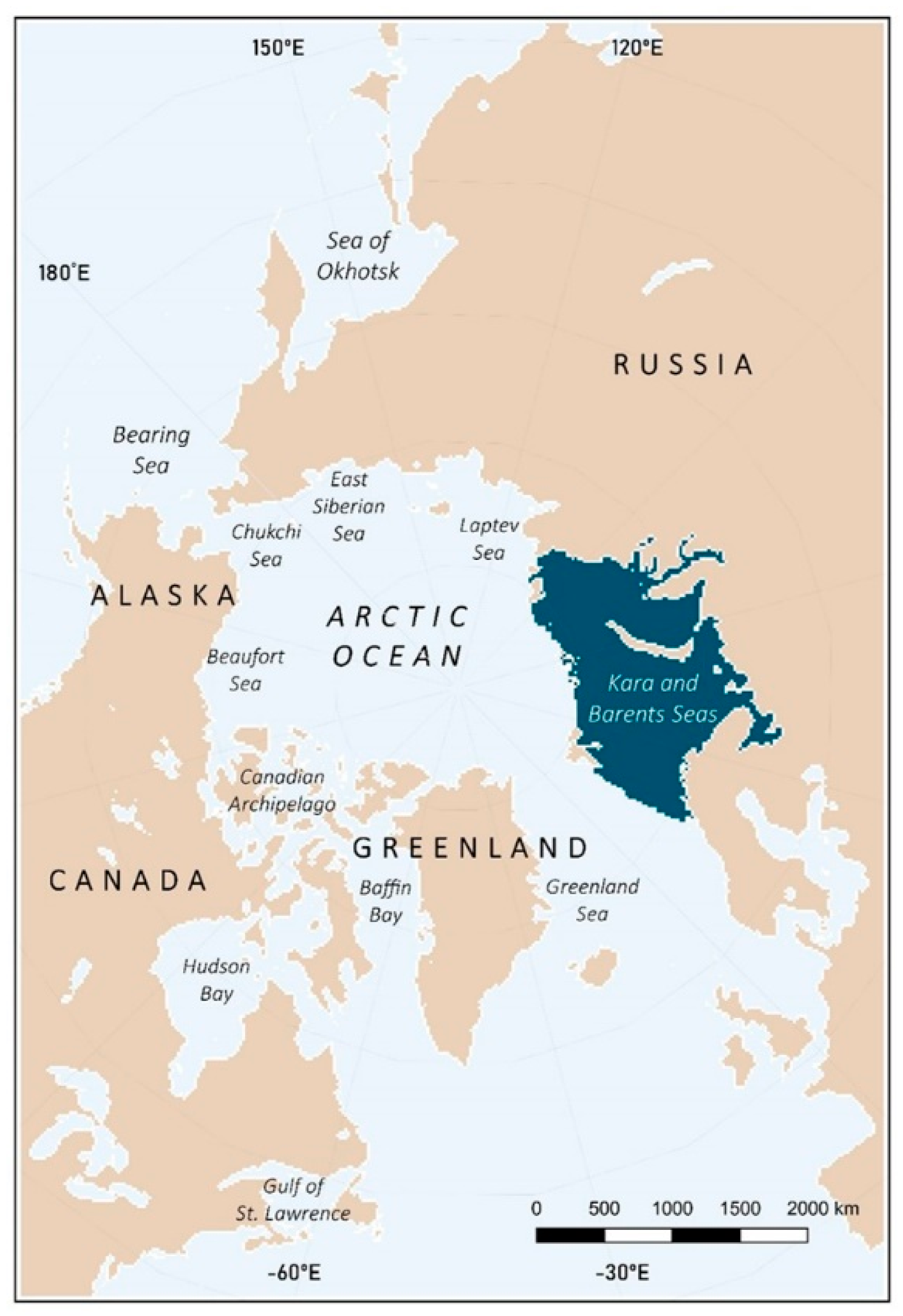
The National Snow and Ice Data Center (NSIDC) provides a region mask for the Arctic, which includes nine seas: The Seas of Okhotsk and Japan, Bering Sea, Hudson Bay, Baffin Bay/Davis Strait/Labrador Sea, Greenland Sea, Kara and Barents Seas, Arctic Ocean, Canadian Archipelago, and Gulf of St. Lawrence. We selected the Kara and Barents Seas as our study area, and 4076 grid points at a resolution of 25 km were extracted from the region mask (Figure 1). The Kara Sea is part of the Arctic Ocean on the north coast of Russia, and is located between Novaya Zemlya and Severnaya Zemlya. The Barents Sea is surrounded by the Svalbard Islands to the northwest, the Franz Josef Islands to the northeast, and the Novaya Zemlya Islands to the east. The sea ice area of the Kara and Barents Seas usually begins to decrease sharply between June and August, reaching its minimum in September, and begins to freeze in October, peaking in April. The Kara and Barents Seas represent a key area of Arctic sea ice shift [11] as warm Atlantic waters flow into the Arctic Ocean [12]. The Kara and Barents Seas have a highly variable SIC which is strongly influenced by the North Atlantic oscillation [13]. Such changes in sea ice play an important role in establishing a new relationship between the atmosphere and sea ice under conditions of Arctic warming [14]. In particular, the Barents Sea is an important area affecting the variation of the entire Arctic air–ice–ocean system [15]. Sato et al. [16] mentioned that apparent links between the Barents Sea ice coverage and the cold Eurasian winters are associated with part of a teleconnection pattern which originates from outside the Arctic. The remote planetary wave atmospheric response to the poleward shift of a sea surface temperature over the Gulf Stream would be amplified over the Barents Sea region via interacting with the sea ice anomaly, promoting the warm Arctic and cold Eurasian pattern. In addition, the sea ice decline in the Kara and Barents Seas is related to the Ural Blocking (UB) and North Atlantic Oscillation+ (NAO+) at the same time, and is followed by the warm Arctic–cold Eurasian (WACE) pattern. The existence of a long-lived UB event can lead to additional warming of the Kara and Barents Seas through the emergence of a persistent quasi-biweekly WACE (QB-WACE) anomaly event and amplifies the warming of the Kara and Barents Seas before UB begins to establish a strong winter (DJF) average WACE pattern, resulting in a loss of sea ice to the Kara and Barents Seas [17].
2.2. Sea Ice Concentration Data
We used the Climate Data Record (CDR) dataset of passive microwave sea ice concentration provided by the National Oceanic and Atmospheric Administration (NOAA) NSIDC. Microwave sensors play an important role in monitoring sea ice conditions during polar nights and in the presence of clouds when optical and infrared sensors fail. The Electrically Scanning Microwave Radiometer (ESMR), developed in 1973, was the first microwave sensor to monitor sea ice and was replaced by the Scanning Multichannel Microwave Radiometer (SMMR) in 1978. From 1987 to 2007, the Special Sensor Microwave Imager (SSM/I) was operated for the F8, F11, and F13 flights of the Defense Meteorological Satellite Program (DMSP). SSM/I was replaced by SSMIS (Special Sensor Microwave Imager/Sounder) onboard DMSP F17. The SMMR, SSM/I, and SSMIS observational records have provided continuous SIE and SIC values for over 30 years [18] (Table 1). The NASA Goddard Space Flight Center (GSFC) provides merged sea ice concentration data, using the NOAA CDR algorithm to produce consistent data over a long period of time. The product is a rule-based combination of SIC estimates from two well-established algorithms: the NASA Team algorithm [19] and the NASA Bootstrap algorithm [20]. These products are provided in the form of monthly average and have a spatial resolution of 25 km with a polar stereographic projection centered on the North Pole (with central meridian of 45°W and standard parallel of 70°N). The SIC value in this product refers to the fraction of sea ice within a certain area. A value of 0 indicates that no ice is present within a pixel, and a value of 1 means that the ice covers the entire pixel. Although the SIC retrieval algorithm has been improved by many efforts, the major error sources are thin ice (30% to 50%) and surface melt (10% to 30%) [21].
2.3. Climate Data
For modeling SIC changes, RCM data provided by the Coordinated Regional Downscaling Experiment (CORDEX) was used. The Arctic CORDEX initiative is an international coordinated framework to produce an improved ensemble of regional climate change projections as the input for impact and adaptation studies aimed at a better understanding of the regional climate in the Arctic [22]. The RCM is based on dynamic downscaling of the GCM, enabling more detailed forecasting in specific regions with improved spatial resolution. Nine databases are available for the RCM in the Arctic region, and Table 2 shows the name, institute of origin, and driving GCM for each database. The period of data used is from January 2006 to December 2030 under the RCP 8.5 scenario assuming that the current emission trend will continue without reduction of greenhouse gas emissions. Regional climate model provides 45 variables in the form of monthly average on a 0.44° grid. We first extracted 19 climatic variables as the factors influencing the Arctic sea ice changes: precipitation, total cloud fraction, near-surface wind velocity, evaporation, near-surface specific humidity, sea-level pressure, near-surface air temperature, duration of sunshine, surface downwelling longwave radiation, surface upwelling longwave radiation, top of atmosphere (TOA) outgoing longwave radiation, surface upwelling shortwave radiation, TOA incident shortwave radiation, surface upwelling shortwave radiation, TOA outgoing shortwave radiation, surface upward latent heat flux, and surface upward sensible heat flux.
Using a spatial collocation procedure by the nearest neighbor method for the SIC and RCM datasets, correlation coefficients between SIC and the 19 extracted climate variables were investigated. We calculated the generic correlation coefficients irrespective of spatial or temporal context because we needed to select several appropriate variables from the 19 RCM variables, which can represent for all the years and months, and all the grid points. Finally, four climate variables with absolute values of correlation coefficients that were 0.5 or greater were selected as input variables for our prediction model (Table 3): near-surface air temperature (TAS), near-surface specific humidity (HUSS), surface downwelling longwave radiation (RLDS), and surface upwelling longwave radiation (RLUS). To avoid the redundancy problem of the input variables, a multicollinearity test was carried out for the four variables (TAS, HUSS, RLDS, and RLUS) using the variance inflation factor (VIF), which showed no severe multicollinearity. Near-surface specific humidity refers to the mass of water vapor per unit mass of moist air and is usually expressed in units of g/kg or kg/kg. As the specific humidity in the atmosphere increases, atmospheric moisture fluxes increase, whereas when the sea ice cover decreases, the air–sea moisture flux tends to increase. [23]. According to Kim et al. [24], the magnitude of winter specific humidity increases by 0.037 g/kg per 1% reduction in sea ice concentration of the Kara and Barents Seas. Recently, the temperature in the Kara and Barents Seas increased by 0.94 °C ± 0.9 °C over 10 years, and the SIE decreased by approximately 107 km2 [25]. The correlation between SIC and downward longwave radiation in the Barents Sea was significant in winter and summer, and moisture transport through this region was accompanied by longwave radiation changes and SIC variations [26]. Over most of the Barents Sea, the surface heat flux trend is strongly downward, that is, a turbulent heat transfer trend from the atmosphere to the ocean. In the Kara Sea, the heat flux trend is upward, presumably reflecting the effect of declining sea ice cover and ice thickness. This upward heat flux trend could be caused by ocean warming during the sunlit season when ice–albedo feedback can contribute to the warming [27].
2.4. Reference Data
For reference data on the four climate variables (TAS, HUSS, RLDS, and RLUS) from RCMs, we used the spatially interpolated version of ERA-Interim data on a 0.4° grid, as well as the Clouds and the Earth’s Radiant Energy System Energy Balanced and Filled (CERES-EBAF) data on a 1° grid. The variable HUSS is not included in the ERA-Interim product, but dew point temperature is, so we used the dew point temperature and surface pressure instead. To calculate HUSS, the vapor pressure, e (hPa), was derived from the dew point temperature, Td (°C):
e = 6.112 × exp[(17.67 × Td)/(Td + 243.5)].
When the vapor pressure (e) and pressure (p) are known, specific humidity (q) is calculated as
q = (0.622 × e)/[p − (0.378 × e)].
As references for the variables RLDS and RLUS, we used the data for downwelling longwave flux and surface upwelling longwave flux included in the surface product from CERES-EBAF. The CERES instruments onboard the Terra and Aqua satellites have been in operation since December 1999 and May 2002, respectively, monitoring the Earth’s reflected and emitted radiation [28].
3. Methods
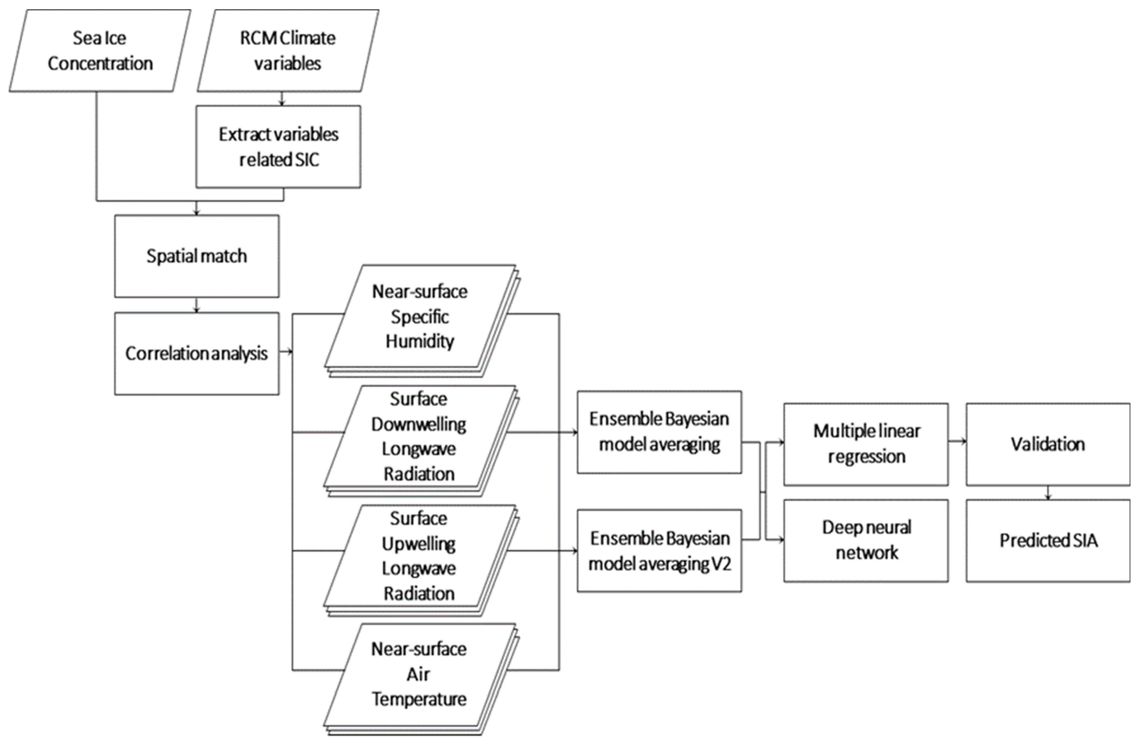
The BMA method was employed to mitigate the uncertainty problem that arises when using a single RCM. For SIC modeling, DNN is used to deal with the non-linear relationships and future predictions. Figure 2 shows the overall flow of database preparation, and model training and validation.
3.1. Bayesian Model Averaging
BMA is a statistical ensemble technique that solves the uncertainty problem in model data by setting different weights for each member based on the posterior probability [10]. For example, we determine the ensemble value for the variable y (reference or true data) using the BMA of k models. In our case, nine RCMs were used as ensemble member, and ERA-Interim and CERES-EBAF were used as reference data. When the value of each member is denoted as , and its bias-corrected value is expressed as , and the theoretical formula for BMA is
where is the weight of each member and is a probability density function for the bias-corrected forecast of each member , which follows a normal distribution. The weight and the variance of the normal distribution can be derived using the expectation-maximization (EM) algorithm, a parameter optimization technique. In the expectation (E) step of the EM algorithm, a log likelihood function is calculated from a given parameter set. In the maximization (M) step, a parameter set is derived to maximize this log likelihood function. The E and M steps are repeated to derive the optimal parameters (i.e., the weight of each member and the variance of the normal distribution) until the log likelihood function converges on a maximum value. A weighted average of the BMA approximation is calculated using the weight of each member derived from the EM algorithm:
We conducted spatial collocation analysis for the four climate variables using the reference data and the nine RCMs representing the period between January 2006 and December 2016. A total of 538,032 (11 years × 12 months × 4,076 grid points) match-ups were constructed, and the BMA ensemble value was calculated using these match-ups.
3.2. Multiple Linear Regression
MLR is used to establish a linear combination of relationships between multiple explanatory variables x (HUSS, RLDS, RLUS, and TAS), and the response variable y (SIC). We built an MLR model using SIC data and the four climate variables for 132 months from January 2006 to December 2016.
We used a BMA ensemble as well as a single RCM to determine the explanatory variables (HUSS, RLDS, RLUS, and TAS).
3.3. Deep Neural Network
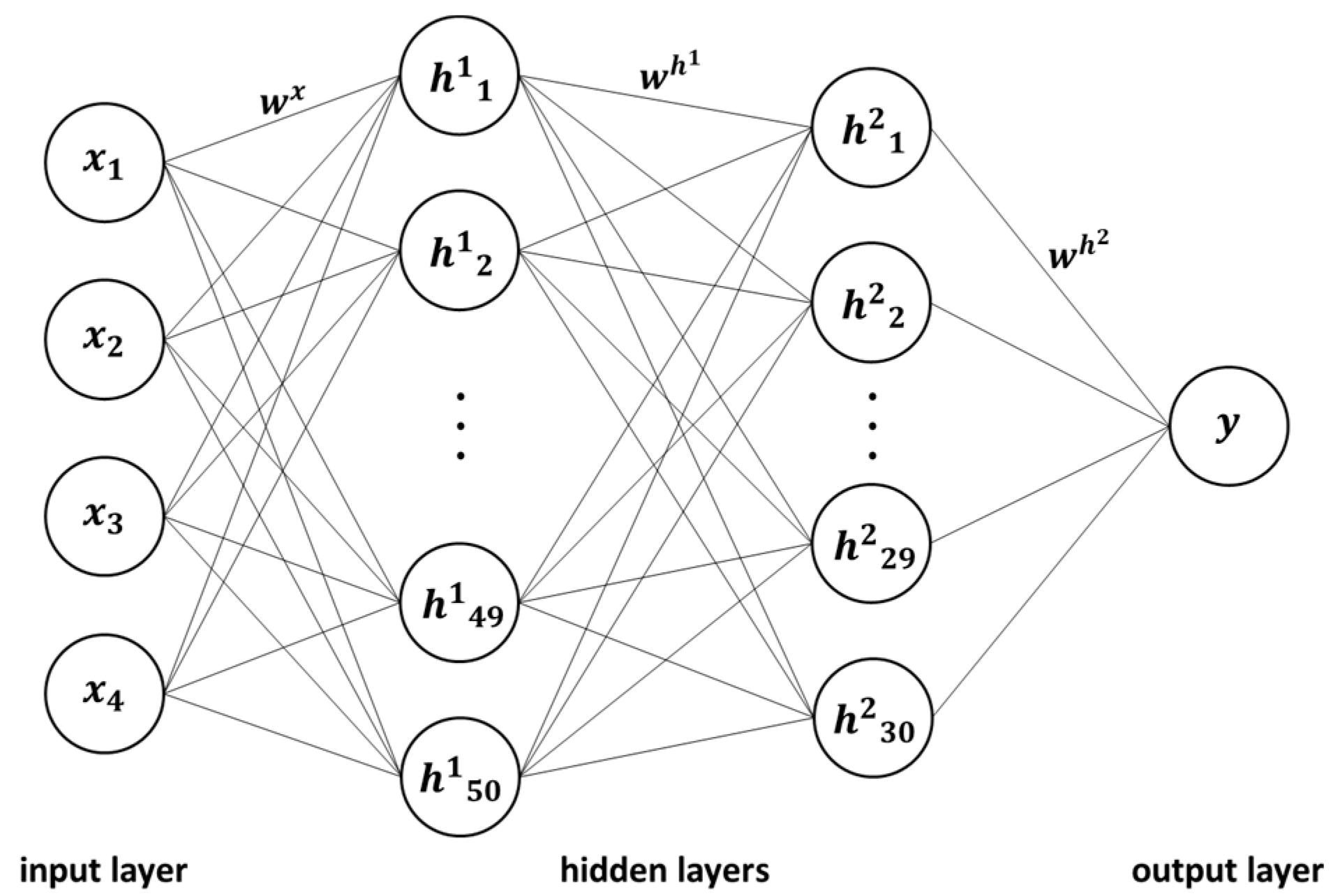
The classic MLP neural network method has a local minimum problem in which an optimization process often stops at a locally optimized state, rather than a globally optimized state. Moreover, general machine learning methods sometimes reveal an overfitting problem that cannot handle actual data containing outliers due to excessive learning based only on the given dataset. Such problems can be solved with a DNN through an optimization algorithm in the intensive deep network (Figure 3). Backward optimization and forward optimization were both conducted using the back-propagation algorithm for improved accuracy. The vanishing gradient problem of a loss function, which may occur during back-propagation, can be fixed by applying appropriate activation functions.
We constructed a DNN model using data from January 2006 to December 2016. To determine an optimal layer structure, we conducted two-step experiments. We first tested the model structure with [10, 10], [30, 30], [50, 50], [100, 100], and [200, 200] neurons, and found that [50, 50] was best among them, although they showed very little difference. Then, we tested the models with [50, 30], [50, 10], and [50, 30, 10] neurons, and the model with [50, 30] neurons produced the best performance in the training, where the mean square error (MSE) was used for the loss function. For each epoch and iteration, we used an Adaptive Delta (ADADELTA) optimizer to minimize the loss function by adjusting a set of weights and biases in the neural network. ADADELTA is a stochastic gradient descent algorithm that obtains the gradient of the loss function from a stochastically selected dataset, rather than the entire dataset. It is less sensitive to hyperparameters and has the advantage of preventing the learning rates from decreasing too quickly. In addition, we used a rectified linear unit (ReLU) activation function to avoid the vanishing gradient problem. In the case of MLR, multi-collinearity among input variables may cause regression coefficients to change erratically in response to small changes in the data, similar to the overfitting problem. In order to deal with the weak multi-collinearity which may remain in the input variables, we added L1/L2 regularization in our DNN model. The L1-regularized loss function can secure the sparsity of a model and the L2-regularized loss function can ensure the simplicity of a model. We used the least absolute shrinkage and selection operator (LASSO) for the L1 regularization and the ridge regression for the L2 regularization.
4. Results and Discussion
4.1. Multi-Model Ensemble
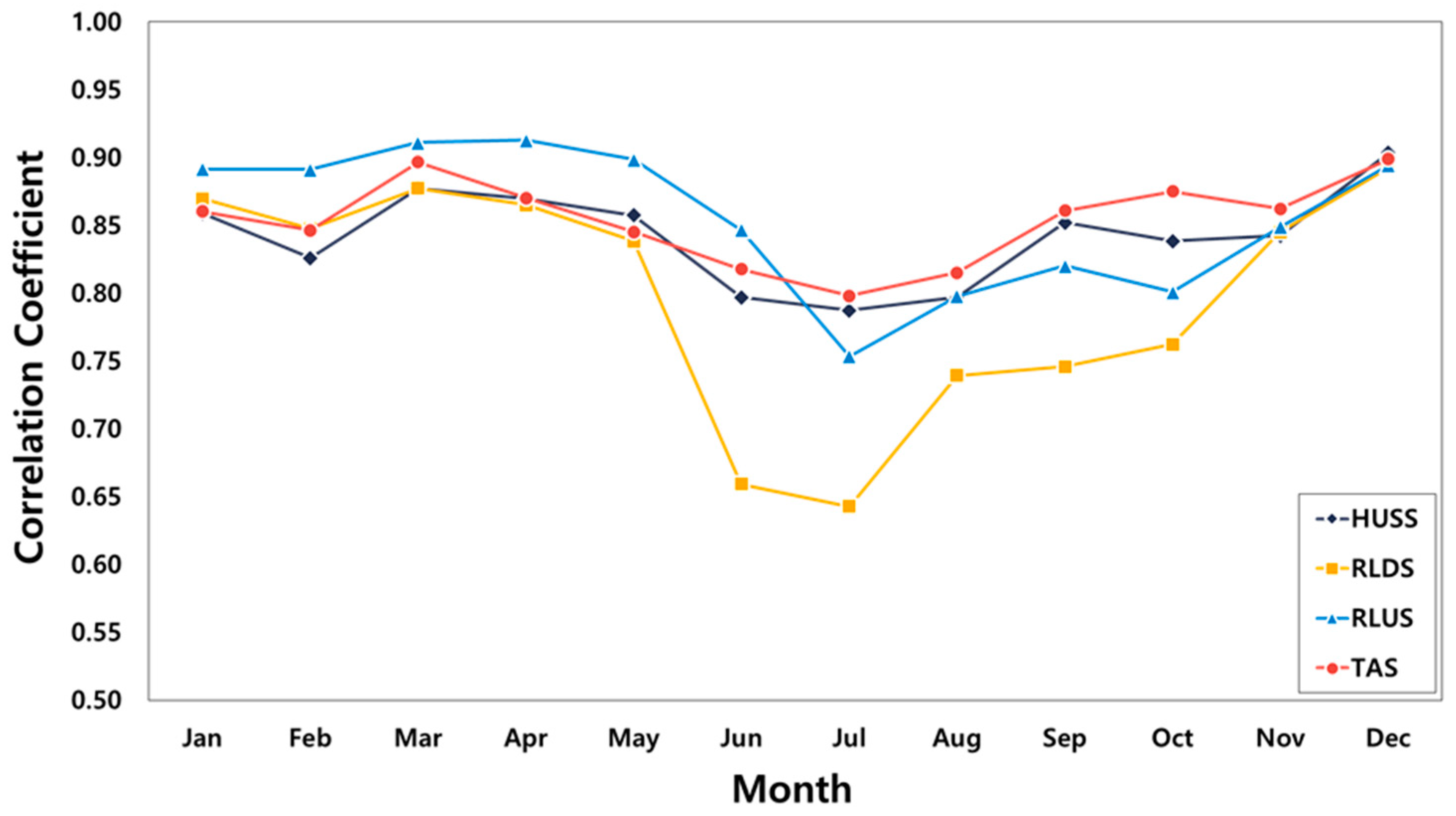
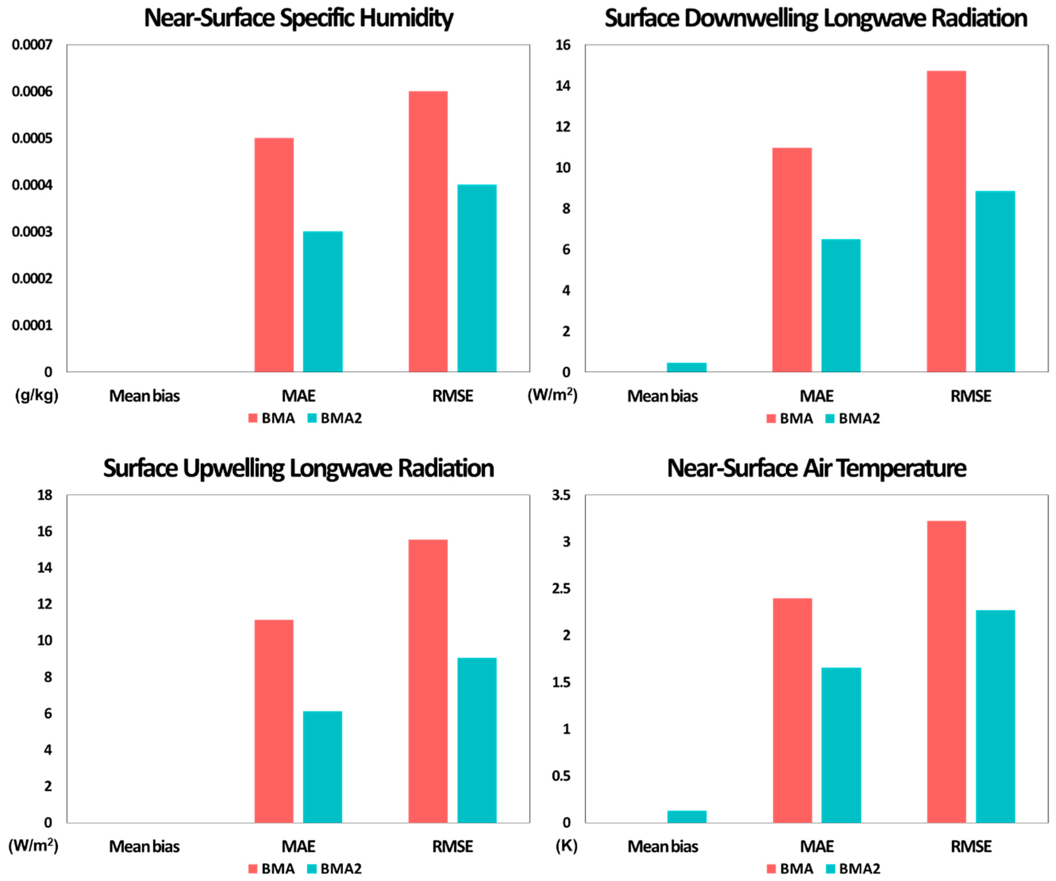
The correlation coefficients between the input variables and their reference data were improved with the BMA, from approximately by 0.03 to 0.05 for HUSS, TAS, RLDS, and RLUS, when compared with the average of the nine RCMs (Table 4). However, the seasonal variation of the climate variables was significant due to differences in the amount and duration of solar radiation in the Arctic during summer and winter. Therefore, we examined the seasonal characteristics of the monthly correlation coefficients of the BMA (Figure 4) and found that the correlation coefficients of all variables decreased in summer (May to August). In addition, the spatial coverage of the Arctic region is very large and, thus, the BMA should be adjusted to deal with both the spatial and temporal variations in climate variables. Therefore, we employed the BMA2 method which extracts BMA weights by month and by grid point. To take into account the spatial and temporal characteristics, we divided all match-ups (538,032 grid points) into 12 months, and then into 4076 grid points to calculate the BMA weights for each member. The leave-one-year-out (also known as jackknife) method was used for training and validation of the BMA2 ensemble. Training was conducted using a 10-year dataset, excluding one year, and the validation was carried out for the excluded year. Such tests were iterated 11 times for each year between 2006 and 2016. The averaged error statistics of the BMA2 is shown in Table 4 and Table 5. The mean absolute error (MAE) and RMSE of BMA2 improved markedly for all variables, with a correlation coefficient of approximately 0.97 (Figure 5). Compared with the RCMs, the correlation coefficients were improved by 0.07 for HUSS and TAS and by 0.1 for RLDS and RLUS. All the p-values were 0, which indicates the statistical significance of the correlation coefficients. Accordingly, the climate variables created by BMA2 were used as input data for our SIC prediction model.
4.2. Prediction of Sea Ice Concentration
We first built prediction models using MLR and the DNN from the match-ups used for SIC and climate variables obtained from a single RCM (MGO-RRCM) between January 2006 and December 2016. The leave-one-year-out method was used for training and validation. The prediction model was trained using a 10-year dataset excluding one year, and the predicted values for the excluded year were compared with the true values. For example, the predicted values for the period 2006–2015, excluding the year 2016, were validated using 2016 data. In this way, 11 sets of training and validation were carried out for each year (2006, 2007, …, 2016), and Table 6 summarizes the validation statistics. The MLR with a single RCM had a correlation of 0.719, and the correlation was improved when using the DNN model (r = 0.766). The correlation was even more improved further by using the DNN with the BMA2 ensemble (r = 0.888). Compared with MLR, the correlation of the DNN increased by 0.047 (0.766−0.719). Additionally, the correlation of DNN with the BMA2 ensemble increased by 0.122 (0.88−0.766) compared with DNN and a single RCM. Finally, DNN with the BMA2 ensemble exhibited a synergistic advantage of 0.169 (0.888−0.719) compared with the generic MLR. These results indicate that correlation was improved by combining the optimal input data (BMA2) with the optimal non-linear model (DNN). All p-values were 0, which indicates the statistical significance of the correlation coefficients.
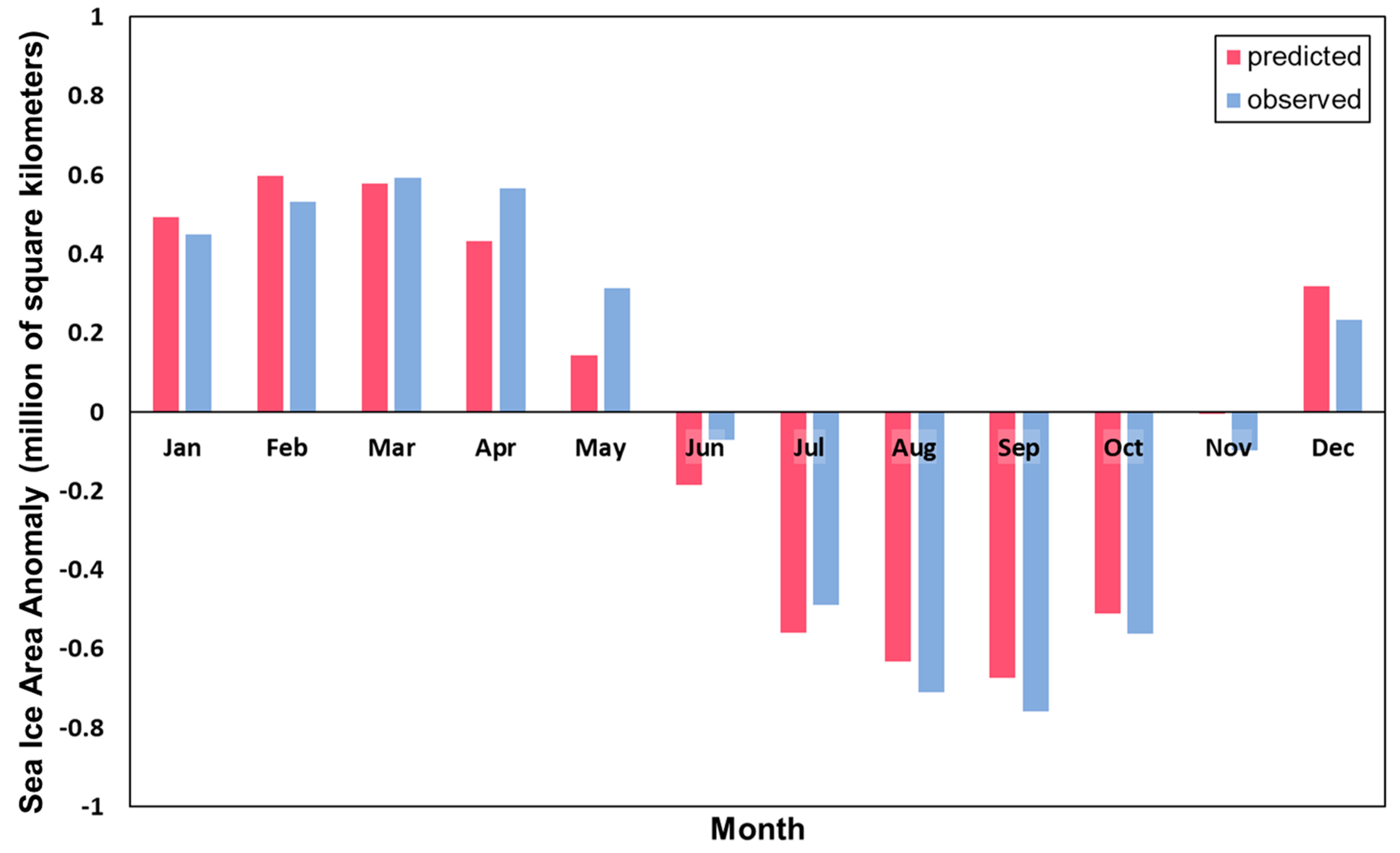
Since long-term changes in sea ice can exhibit seasonality [29], we examined the monthly characteristics of the validation statistics of the DNN with BMA2 ensemble. Figure 6 shows the eleven-year (2006–2016) averages of the monthly anomalies of the sea ice concentration from satellite observations and the predictions of the DNN with BMA2 ensemble. From November to May, when sea ice is growing, the model showed high correlation coefficients, but relatively low correlations were found in the melting season from June to October (Table 7). In August and September, when sea ice was mostly melted, the correlation was lowest (0.467 and 0.384, respectively). Although a low correlation coefficient is generally accompanied by high RMSE, the RMSE of the prediction model was also low (0.145 and 0.121, respectively), because the sea ice of the Kara and Barents Seas in August and September has a very low SIC value of zero or nearly zero. Therefore, we calculated the normalized RMSE (NRMSE), which can be calculated by dividing the RMSE by the standard deviation to represent error normalized according to the range of the values. The NRMSE showed the opposite trend to that of the correlation coefficient, which allows an intuitive understanding of the error characteristics. Low prediction accuracy in summer presumably occurs because thin summer ice is more sensitive to variations in atmospheric conditions [30,31]. In addition, the decline in summer snowfall due to the shift from snowfall to rainfall has greatly increased the fraction of bare sea ice and melt ponds with much lower albedo than snow-covered sea ice, likely contributing to the thinning of sea ice in recent decades [32]. In addition to thermodynamic conditions, thin ice is more sensitive to wind forcing, which is observed as increased ice drift speeds [33,34].
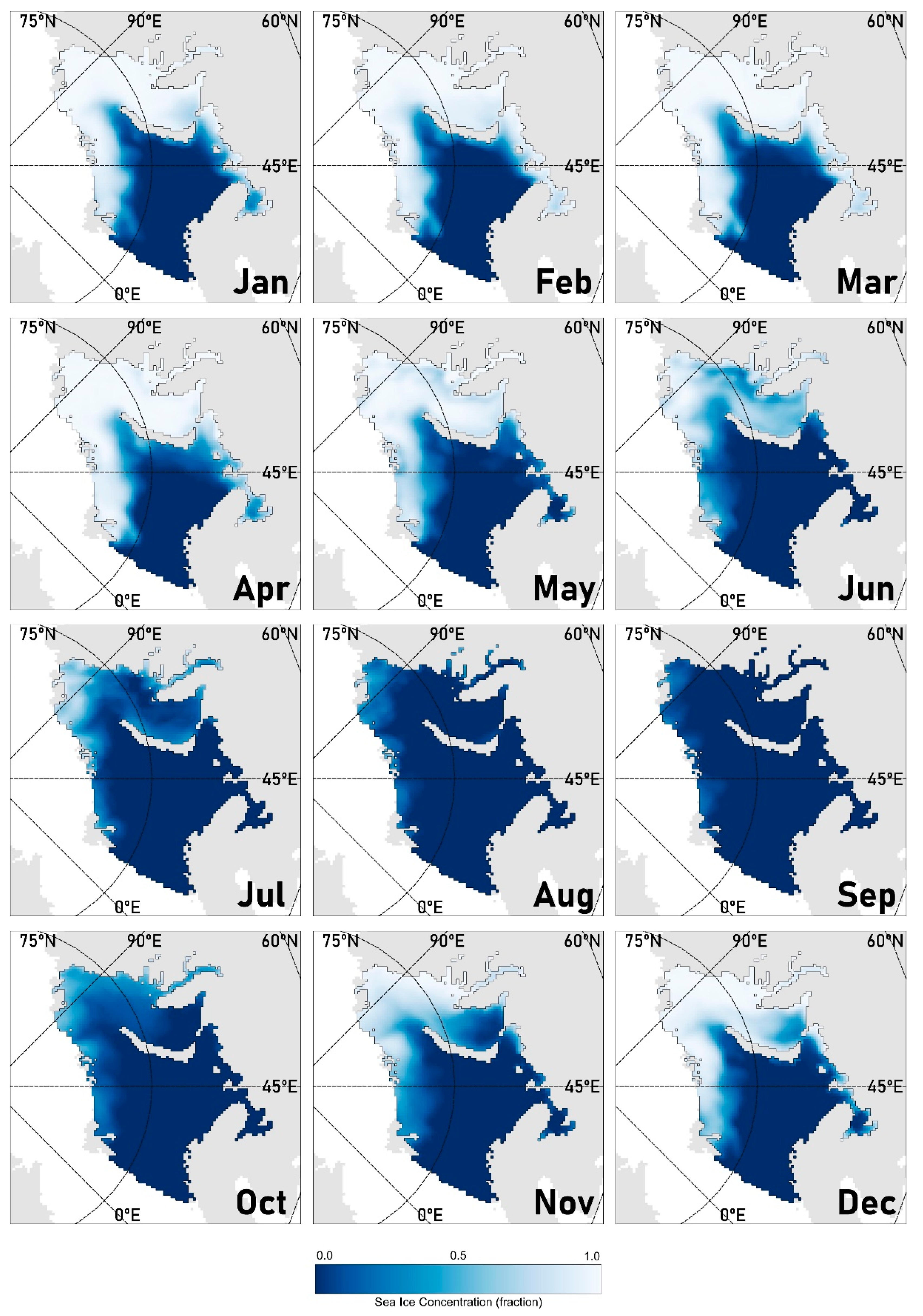
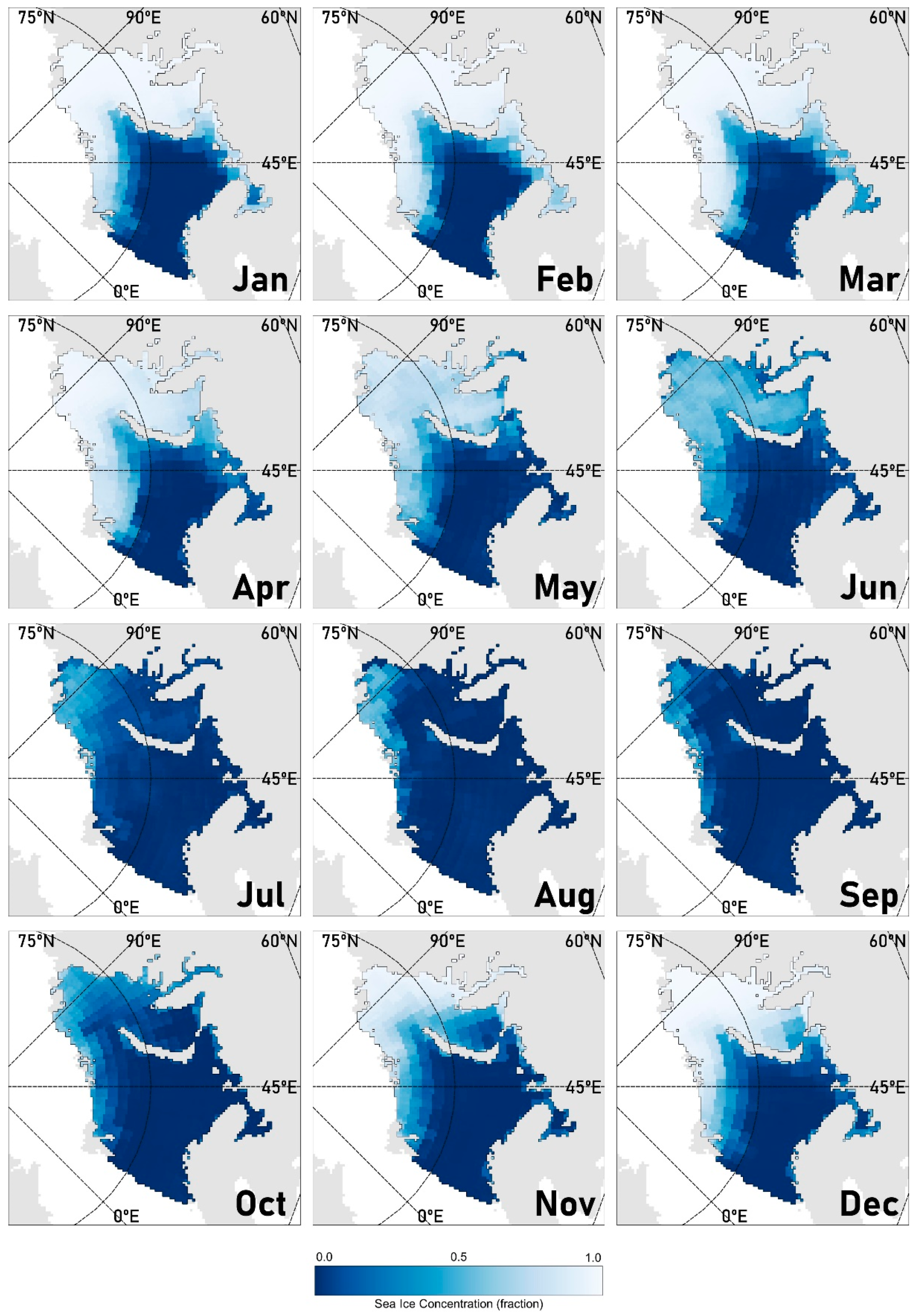
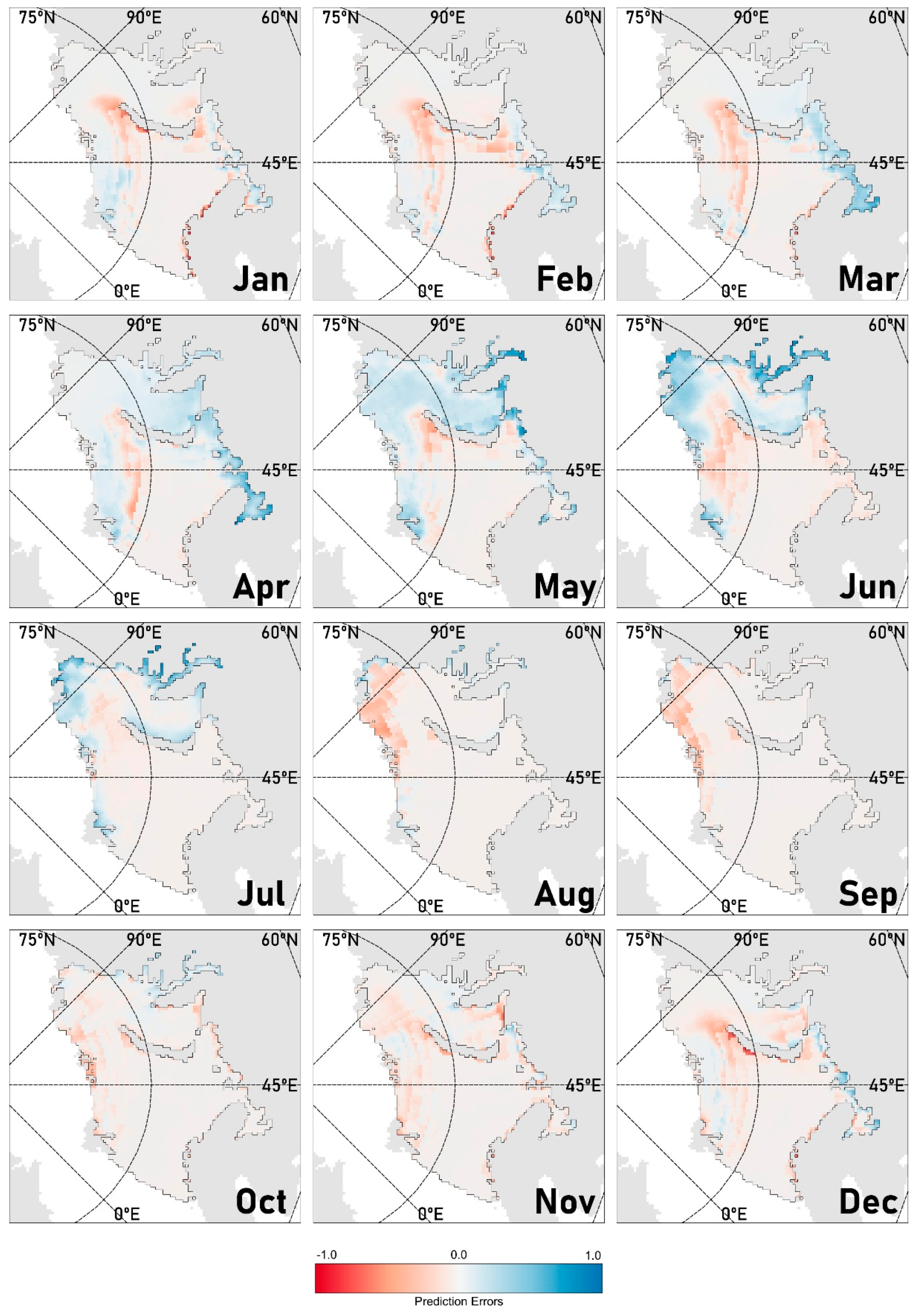
Figure 7 shows monthly satellite observations of SIC and Figure 8 shows the predictions of the DNN with BMA2 ensemble for the period 2006–2016. Each of these figures uses the 11-year averages for each pixel. Figure 9 shows the difference between the observations and predictions, with overestimation indicated in red and underestimation in blue. High SIC had a tendency to be underestimated, while low SIC seemed to be often overestimated. It is probably because of the conservative behavior of the prediction model to optimize the loss function. Such an error distribution is stronger in spring and summer. In particular, overestimation was vague at the boundary between the sea ice and open ocean. Warm and salty Atlantic Water flows into the Barents Sea through the Barents Sea Opening (BSO) and meets the cold Arctic water, resulting in a polar front. The uncertainty of SIC prediction can be affected by this polar front, which is located close to the boundary between the sea ice and open ocean [35]. In addition, coastline pixels showed relatively large errors due to the mixed pixel problem, which occurs when land and sea are both included in a pixel. Since coastline can be influenced by meteorological phenomena that occur over land, the errors can increase when the surface temperature changes drastically between the coastline and inland area.
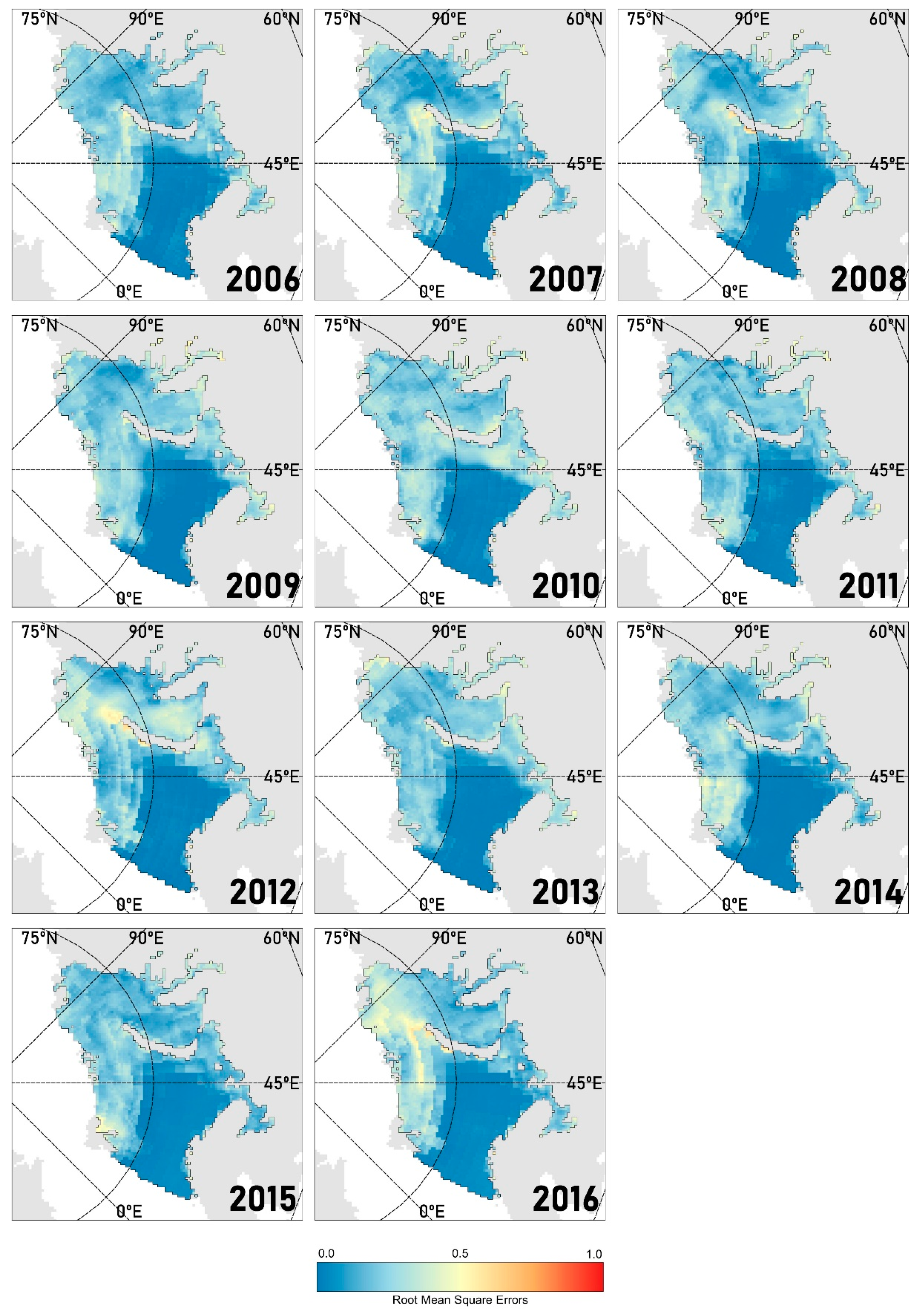
In light of recent trends in the decrease of Arctic sea ice due to global warming, we examined the time-series characteristics of SIC prediction (Table 8). The accuracy was quite high, with a correlation coefficient of over 0.87 for most years. The correlation was slightly lower in 2012 and 2016 (0.85 and 0.858, respectively) with a pattern of underestimation, which means that sea ice melted more than expected, especially in 2012 and 2016. Indeed, in September 2012 and 2016, Arctic SIE reached its minimum since satellite observation began. In 2012 and 2016, the Kara and Barents Seas began to melt three to four weeks earlier than the other years. The decrease in surface albedo caused by such early melting accelerated the melting process through absorption of more solar radiation [36]. Hence, we assume that the prediction errors for these two years were partly because of the earlier melting. Figure 10 is a map showing yearly RMSE for the period between 2006 and 2016. The error is relatively large in shallow areas north of Novaya Zemlya. The North Atlantic Current, which flows through the BSO, is transformed into Circumpolar Deep Water (CDW) below 0 °C through cooling and mixing due to wind and cold atmosphere [18,37]. Heat energy in the transformed current decreases gradually as it flows to the Arctic Ocean through the strait between the Novaya Zemlya and Franz Josef Islands [37]. These unique regional characteristics were not taken into account in our prediction model, resulting in a partly lower performance.
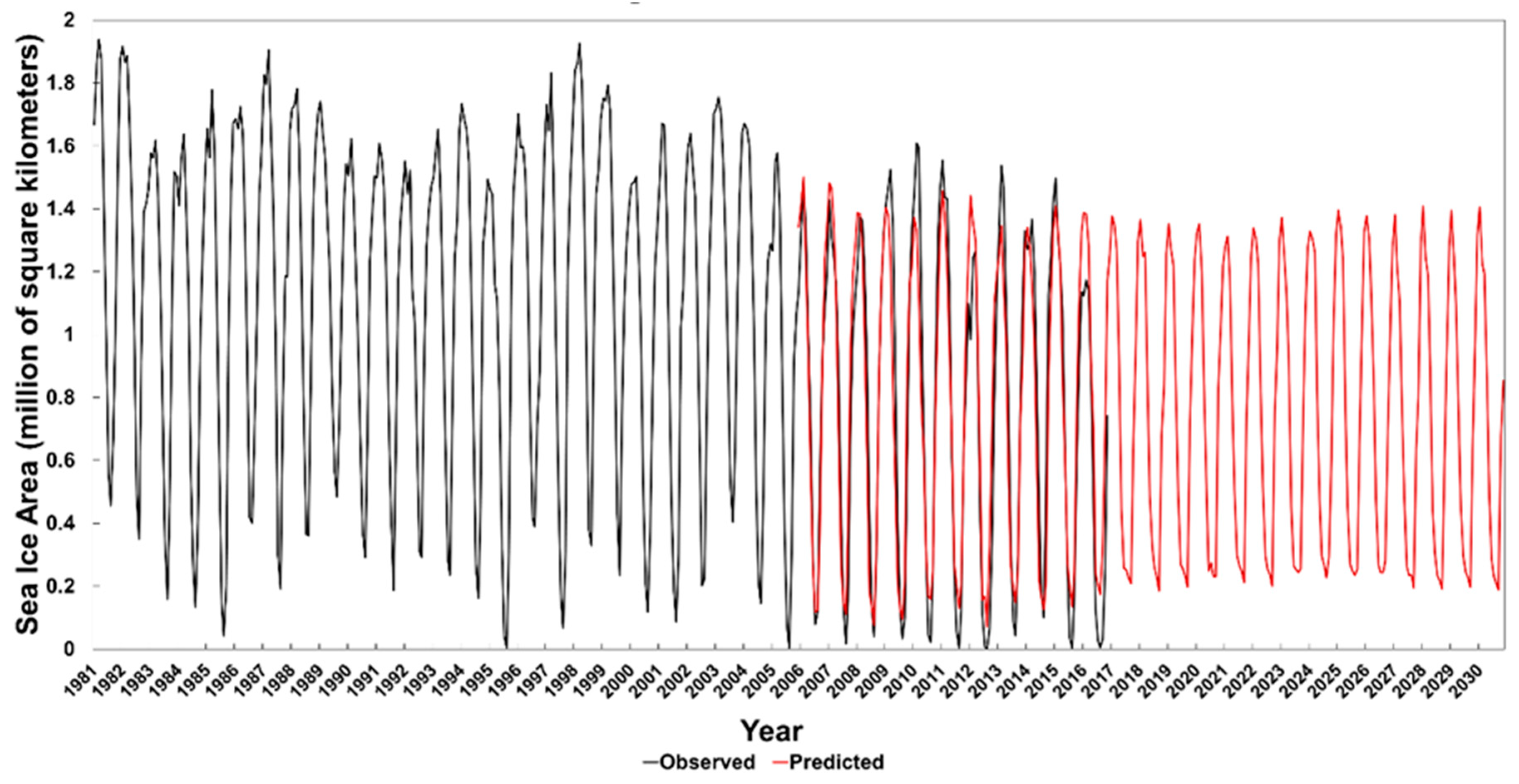
Figure 11 shows the time-series change in monthly averages of sea ice area (SIA), the sum of the area covered by sea ice, for the period 1981–2030. The SIA is defined by multiplication of SIC and the area size of a pixel. The black dotted line denotes satellite observations, and the red solid line represents values predicted by our DNN with BMA2 ensemble. The prediction accuracy for 2017–2030 is similar to that for 2006–2016 (r = 0.884). SIA appears to decline continuously over the next 10 years (2017–2030), but its decrease may be slower than during the period before 2016. Indeed, the RCMs did not show sensitive change after 2017, which leads to the small variation of the SIC for the period 2017–2030.
Over parts of the Kara Seas, where the surface heat flux trend is upward and with a larger magnitude than the downward infrared radiation trend, it is possible that the positive surface air temperature trend arises from an upward sensible and/or latent heat flux, as well as an increase in the downward infrared radiation due to the input of additional water vapor into the atmosphere. It was shown that the downward infrared radiation trend is associated with a trend in the moisture fluxes from mid-latitudes into the Arctic, as well as a trend in the total column liquid water and ice in the Arctic [27]. Gong and Luo [38] showed that a long-term increase in the intraseasonal moisture intrusions into the Arctic can help account for the positive trend in the downward infrared radiation during the winter season over recent decades. An increase in low- and mid-latitude moisture and the moisture fluxes into the Arctic are an important contributor to the downward infrared radiation trend poleward of 70°N. More moisture intrusion into the Kara and Barents Seas seems to result in enhanced downward infrared radiation and, in turn, stronger warming [39]. That is, the combined UB and NAO+ patterns results in a cooperative circulation pattern conducive to strong decline of sea ice through strong warming of Kara and Barents Seas due to strong downward infrared radiation associated with increased water vapor.
Recent climate changes have lead to a transition from the cold and stratified Arctic to the warm and well-mixed Atlantic. The Barents Sea, which is the gateway between the Atlantic and the Arctic ocean, has two climatic regimes: a cooler Arctic with fresher water in the North and a softer Atlantic with saltier water in the South. This warming is particularly stronger in the North of the Kara and Barents Seas, which allows the heat from the Atlantic water to remain on the surface and slow the formation of ice in the winter [40]. However, due to the mixing of warm and salty Atlantic water and cold and fresh Arctic water, the upper layers became saltier, which prevents the formation of ice. Therefore, the variability and uncertainty in the sea ice change become more complicated.
5. Conclusions
Indeed, we are dealing with an environment where background conditions are changing rapidly. Hence, the relative importance of the relevant physical processes may be changing, and the linear algorithms based on historical data may not apply in future scenarios. In this context, we presented a near-future prediction of Arctic SIC between 2017 and 2030 based on integration of an advanced RCM ensemble and an optimized DNN model. The accuracies of the RCM variables (TAS, HUSS, RLDS, and RLUS) were greatly improved with the BMA2 method, which considered temporal and spatial variations in order to minimize the uncertainty of individual RCMs. The DNN was used to deal with the non-linear relationships between SIC and climate variables, and to provide a near-future prediction for the next 10–20 years. We adjusted the DNN model for optimized SIC prediction by adopting a best-fitted layer structure, loss function, optimizer algorithm, and activation function. Accuracy improved greatly when the DNN model was combined with the BMA2 ensemble, with a correlation coefficient of 0.888.
The accuracy in the melting season (June to October) was somewhat lower than that in the freezing season (November to May), presumably due to the influence of thinning of sea ice. In summer, thin ice is more sensitive to the effects of atmospheric conditions. In addition, the influence of currents and tides and the locations of polar fronts should be considered in future research. Gradual thinning of sea ice from the past represents sea ice memory [41], and suggests that a time-series approach must be integrated into DNN modeling. As future work, the use of additional, appropriate variables will be necessary for accuracy improvement of the DNN model. Principal component (PC) analysis will be another useful approach. Several PCs can be used as input variables for the DNN model, instead of using the climate variable itself. Also, Fourier analysis of the time-series SIC can be conducted to see whether there are any other periodic patterns in addition to the annual variation, which will facilitate the prediction. The important climate change effects, such as UB/NAO, downward longwave radiation, and Atlantification, should be examined in terms of regional scale. This paper, which is for prediction at a pixel-by-pixel level, did not cover the regional-scale climate effects, but they will provide a clue to solve the uncertainty problem in the Arctic SIC prediction.
Author Contributions
Research design and supervision by Y.-W.L.; data processing and analysis by J.K. and K.K.; Manuscript preparation by J.K. and J.C.; literature review and discussion by Y.Q.K. and H.-J.Y.
Funding
This research was funded by the Pukyong National University Research Abroad Fund in 2014.
Conflicts of Interest
The authors declare no conflict of interest.
References
- Intergovernmental Panel on Climate Change (IPCC). Climate Change 2014: Synthesis Report. Contribution of Working Groups I, II and III to the Fifth Assessment Report of the Intergovernmental Panel on Climate Change; IPCC: Geneva, Switzerland, 2014. [Google Scholar]
- Curry, J.A.; Schramm, J.L.; Ebert, E.E. Sea ice-albedo climate feedback mechanism. J. Clim. 1995, 8, 240–247. [Google Scholar] [CrossRef]
- Stroeve, J.; Frei, A.; McCREIGHT, J.; Ghatak, D. Arctic sea-ice variability revisited. Ann. Glaciol. 2008, 48, 71–81. [Google Scholar] [CrossRef]
- Tivy, A.; Howell, S.E.; Alt, B.; Yackel, J.J.; Carrieres, T. Origins and levels of seasonal forecast skill for sea ice in Hudson Bay using canonical correlation analysis. J. Clim. 2011, 24, 1378–1395. [Google Scholar] [CrossRef]
- Drobot, S.D.; Maslanik, J.A.; Fowler, C. A long-range forecast of Arctic summer sea-ice minimum extent. Geophys. Res. Lett. 2006, 33, L10501. [Google Scholar] [CrossRef]
- Walsh, J.E. Empirical orthogonal functions and the statistical predictability of sea ice extent. In Sea Ice Processes and Models; Pritchard, R.S., Ed.; University of Washington Press: Seattle, WA, USA, 1980; pp. 373–384. [Google Scholar]
- Kim, J.H.; Joeng, J.H.; Kim, B.M.; Shin, J.H. Mid-Long Term Prediction of Arctic Sea Ice Concentration using Statistical Method. Master’s Thesis, Chonnam National University, Gwangju, Korea, February 2016. [Google Scholar]
- Ahn, J.; Hong, S.; Cho, J.; Lee, Y.W.; Lee, H. Statistical Modeling of Sea Ice Concentration Using Satellite Imagery and Climate Reanalysis Data in the Barents and Kara Seas, 1979–2012. Remote Sens. 2014, 6, 5520–5540. [Google Scholar] [CrossRef] [Green Version]
- Chi, J.; Kim, H.C. Prediction of Arctic Sea Ice Concentration Using a Fully Data Driven Deep Neural Network. Remote Sens. 2017, 9, 1305. [Google Scholar] [CrossRef]
- Hoeting, J.A.; Madigan, D.; Raftery, A.E.; Volinsky, C.T. Bayesian model averaging: A tutorial. Stat. Sci. 1999, 14, 382–417. [Google Scholar] [CrossRef]
- Yang, X.Y.; Yuan, X.; Ting, M. Dynamical link between the Barents–Kara sea ice and the Arctic Oscillation. J. Clim. 2016, 29, 5103–5122. [Google Scholar] [CrossRef]
- Schauer, U.; Loeng, H.; Rudels, B.; Ozhigin, V.K.; Dieck, W. Atlantic water flow through the Barents and Kara Seas. Deep Sea Res. Part I Oceanogr. Res. Pap. 2002, 49, 2281–2298. [Google Scholar] [CrossRef]
- Sorteberg, A.; Kvingedal, B. Atmospheric forcing on the Barents Sea winter ice extent. J. Clim. 2006, 19, 4772–4784. [Google Scholar] [CrossRef]
- Yang, X.Y.; Yuan, X. The early winter sea ice variability under the recent Arctic climate shift. J. Clim. 2014, 27, 5092–5110. [Google Scholar] [CrossRef]
- Smedsrud, L.H.; Esau, I.; Ingvaldsen, R.B.; Eldevik, T.; Haugan, P.M.; Li, C.; Lien, V.S.; Olsen, A.; Omar, A.M.; Otterå, O.H.; et al. The role of the Barents Sea in the Arctic climate system. Rev. Geophys. 2013, 51, 415–449. [Google Scholar] [CrossRef]
- Sato, K.; Inoue, J.; Watanabe, M. Influence of the Gulf Stream on the Barents Sea ice retreat and Eurasian coldness during early winter. Environ. Res. Lett. 2014, 9. [Google Scholar] [CrossRef]
- Luo, D.; Xiao, Y.; Yao, Y. Impact of ural blocking on winter warm Arctic-cold Eurasian anomalies. Part I: Blocking-induced amplification. J. Clim. 2016, 29, 3925–3974. [Google Scholar] [CrossRef]
- Serreze, M.C.; Barry, R.G. The Arctic Climate System, 2nd ed.; Cambridge University Press: Cambridge, UK, 2014; ISBN 978-1-107-03717-5. [Google Scholar]
- Cavalieri, D.J.; Gloersen, P.; Campbell, W.J. Determination of sea ice parameters with the Nimbus 7 SMMR. J. Geophys. Res. Atmos. 1984, 89, 5355–5369. [Google Scholar] [CrossRef]
- Comiso, J.C. Characteristics of Arctic winter sea ice from satellite multispectral microwave observations. J. Geophys. Res. Oceans 1986, 91, 975–994. [Google Scholar] [CrossRef]
- National Snow and Ice Data Center (NSIDC). Climate Data Record (CDR) Program: Climate Algorithm Theoretical Basis Document (C-ATBD) Sea Ice Concentration. pp. 50–55. Available online: https://nsidc.org/sites/nsidc.org/files/technical-references/SeaIce_CDR_CATBD_final.pdf (accessed on 20 October 2018).
- Akperov, M.; Rinke, A.; Mokhov, I.I.; Matthes, H.; Semenov, V.A.; Adakudlu, M.; Adakudlu, M.; Cassano, J.; Christensen, J.H.; Mariya, A.; et al. Cyclone activity in the Arctic from an ensemble of regional climate models (Arctic CORDEX). J. Geophys. Res. Atmos. 2018, 123, 2537–2554. [Google Scholar] [CrossRef]
- Boisvert, L.N.; Markus, T.; Vihma, T. Moisture flux changes and trends for the entire Arctic in 2003–2011 derived from EOS Aqua data. J. Geophys. Res. Oceans 2013, 118, 5829–5843. [Google Scholar] [CrossRef]
- Kim, K.Y.; Hamlington, B.D.; Na, H.; Kim, J. Mechanism of seasonal Arctic sea ice evolution and Arctic amplification. Cryosphere 2016, 10, 2191–2202. [Google Scholar] [CrossRef]
- Comiso, J.C. Large decadal decline of the Arctic multiyear ice cover. J. Clim. 2012, 25, 1176–1193. [Google Scholar] [CrossRef]
- Boccolari, M.; Parmiggiani, F. Seasonal co-variability of surface downwelling longwave radiation for the 1982–2009 period in the Arctic. Adv. Sci. Res. 2017, 14, 139–143. [Google Scholar] [CrossRef] [Green Version]
- Lee, S.; Gong, T.; Feldstein, S. Revisiting the Cause of the 1989–2009 Arctic Surface Warming Using the Surface Energy Budget: Downward Infrared Radiation Dominates the Surface Fluxes. Geophys. Res. Lett. 2017, 44, 10–654. [Google Scholar] [CrossRef]
- Rutan, D.A.; Kato, S.; Doelling, D.R.; Rose, F.G.; Nguyen, L.T.; Caldwell, T.E.; Loeb, N.G. CERES synoptic product: Methodology and validation of surface radiant flux. J. Atmos. Ocean. Technol. 2015, 32, 1121–1143. [Google Scholar] [CrossRef]
- Simmonds, I. Comparing and contrasting the behaviour of Arctic and Antarctic sea ice over the 35 years period 1979–2013. Ann. Glaciol. 2015, 56, 18–28. [Google Scholar] [CrossRef]
- Stroeve, J.C.; Serreze, M.C.; Holland, M.M.; Kay, J.E.; Malanik, J.; Barrett, A.P. The Arctic’s rapidly shrinking sea ice cover: A research synthesis. Clim. Chang. 2012, 110, 1005–1027. [Google Scholar] [CrossRef]
- Holland, M.M.; Bitz, C.M.; Tremblay, B.; Bailey, D.A. The role of natural versus forced change in future rapid summer Arctic ice loss. In Arctic Sea Ice Decline: Observations, Projections, Mechanisms, and Implications; Geophysical Monograph Series; American Geophysical Union: Washington, DC, USA, 2008; Volume 180, pp. 133–150. [Google Scholar]
- Screen, J.A.; Simmonds, I. Declining summer snowfall in the Arctic: Causes, impacts and feedbacks. Clim. Dyn. 2012, 38, 2243–2256. [Google Scholar] [CrossRef]
- Spreen, G.; Kwok, R.; Menemenlis, D. Trends in Arctic sea ice drift and role of wind forcing: 1992–2009. Geophys. Res. Lett. 2011, 38, L19501. [Google Scholar] [CrossRef]
- Vihma, T.; Tisler, P.; Uotila, P. Atmospheric forcing on the drift of Arctic sea ice in 1989–2009. Geophys. Res. Lett. 2012, 39, L02501. [Google Scholar] [CrossRef]
- Lubinski, D.J.; Polyak, L.; Forman, S.L. Freshwater and Atlantic water inflows to the deep northern Barents and Kara seas since ca 13 14C ka: Foraminifera and stable isotopes. Quat. Sci. Rev. 2001, 20, 1851–1879. [Google Scholar] [CrossRef]
- National Snow and Ice Data Center. Available online: https://nsidc.org/arcticseaicenews (accessed on 11 September 2018).
- Pfirman, S.; Bauch, D.; Gammelsrød, T. The northern Barents Sea: Water mass distribution and modification. In The Polar Oceans and Their Role in Shaping the Global Environment, 85th ed.; Johannessen, O.M., Muench, R.D., Overland, J.E., Eds.; American Geophysical Union: Washington, DC, USA, 1994; pp. 77–94. ISBN 0-87590-042-9. [Google Scholar]
- Gong, T.; Luo, D. Ural blocking as an amplifier of the Arctic sea ice decline in winter. J. Clim. 2017, 30, 2639–2654. [Google Scholar] [CrossRef]
- Luo, B.; Luo, D.; Wu, L.; Zhong, L.; Simmonds, I. Atmospheric circulation patterns which promote winter Arctic sea ice decline. Environ. Res. Lett. 2017, 12, 054017. [Google Scholar] [CrossRef] [Green Version]
- Årthun, M.; Eldevik, T. On anomalous ocean heat transport toward the Arctic and associated climate predictability. J. Clim. 2016, 29, 689–704. [Google Scholar] [CrossRef]
- Blanchard-Wrigglesworth, E.; Armour, K.C.; Bitz, C.M.; DeWeaver, E. Persistence and inherent predictability of Arctic sea ice in a GCM ensemble and observations. J. Clim. 2011, 24, 231–250. [Google Scholar] [CrossRef]
Figure 1.
Map of the study area provided by the National Snow and Ice Data Center (NSIDC).

Figure 2.
Overall flow diagram of this study.

Figure 3.
Structure of the deep neural network (DNN).

Figure 4.
Averages of the correlation coefficients of Bayesian model averaging (BMA) ensemble for each month during 2006–2016. The correlation coefficients of all variables decreased in summer (May to August), particularly for RLDS.
Figure 4.
Averages of the correlation coefficients of Bayesian model averaging (BMA) ensemble for each month during 2006–2016. The correlation coefficients of all variables decreased in summer (May to August), particularly for RLDS.

Figure 5.
Error statistics of BMA and BMA2 for the four input variables. Accuracy of BMA2 was improved markedly with a correlation coefficient of approximately 0.97.
Figure 5.
Error statistics of BMA and BMA2 for the four input variables. Accuracy of BMA2 was improved markedly with a correlation coefficient of approximately 0.97.

Figure 6.
Eleven-year averages of the monthly anomalies of sea ice concentration from satellite observations and the predictions of the DNN with BMA2 ensemble for the Kara and Barents Seas during 2006–2016.
Figure 6.
Eleven-year averages of the monthly anomalies of sea ice concentration from satellite observations and the predictions of the DNN with BMA2 ensemble for the Kara and Barents Seas during 2006–2016.

Figure 7.
Monthly averages of sea ice concentration from satellite observations of the Kara and Barents Seas during 2006–2016.
Figure 7.
Monthly averages of sea ice concentration from satellite observations of the Kara and Barents Seas during 2006–2016.

Figure 8.
Monthly averages of sea ice concentration predicted by the DNN with BMA2 ensemble for the Kara and Barents Seas during 2006–2016.
Figure 8.
Monthly averages of sea ice concentration predicted by the DNN with BMA2 ensemble for the Kara and Barents Seas during 2006–2016.

Figure 9.
Errors of monthly averages of sea ice concentration predicted by the DNN with BMA2 ensemble for the Kara and Barents Seas during 2006–2016.
Figure 9.
Errors of monthly averages of sea ice concentration predicted by the DNN with BMA2 ensemble for the Kara and Barents Seas during 2006–2016.

Figure 10.
Twelve-month averages of root mean square error predicted by the DNN with BMA2 ensemble for the Kara and Barents Seas during 2006–2016.
Figure 10.
Twelve-month averages of root mean square error predicted by the DNN with BMA2 ensemble for the Kara and Barents Seas during 2006–2016.

Figure 11.
Monthly averages of sea ice area from satellite observations (black dotted line) and the predictions by DNN with BMA2 ensemble (red solid line) from 1981 to 2030. The decrease of sea ice after 2016 may be slower than during the period before 2016.
Figure 11.
Monthly averages of sea ice area from satellite observations (black dotted line) and the predictions by DNN with BMA2 ensemble (red solid line) from 1981 to 2030. The decrease of sea ice after 2016 may be slower than during the period before 2016.


Table 1.
Satellite sensors for measuring sea ice concentration since 1978.
| Sensor | SMMR | SMM/I | SSM/I | SSM/I | SSMIS |
|---|---|---|---|---|---|
| Platform | Nimbus-7 | DMSP-F8 | DMSP-F11 | DMSP-F13 | DMSP-F17 |
| Spatial resolution | 25 km | 25 km | 25 km | 25 km | 25 km |
| Operation period | 1978–1987 | 1987–1991 | 1991–1995 | 1995–2007 | 2007–present |
Table 2.
Nine regional climate models (RCMs) available for the Arctic.
| No. | RCM | Institute | Driving GCM | Original Resolution Vertical, Horizontal |
|---|---|---|---|---|
| 1 | RCA4 | Swedish Meteorological and Hydrological Institute (SMHI) | CCCma-CanESM2 | L40, 0.44° |
| 2 | HIRHAM5 | Danish Meteorological Institute (DMI) | ICHEC-EC-EARTH | L31, 0.44° |
| 3 | RCA4 | SMHI | ICHEC-EC-EARTH | L40, 0.44° |
| 4 | RCA4-SN | |||
| 5 | HIRHAM5 | Alfred Wegener Institute Helmholtz Centre (AWI) | MPI-M-MPI-ESM-LR | L40, 0.5° |
| 6 | RRCM | Voeikov Main Geophysical Observatory (MGO) | MPI-M-MPI-ESM-LR | L25, 50 km |
| 7 | RCA4 | SMHI | MPI-M-MPI-ESM-LR | L40, 0.44° |
| 8 | RCA4-SN | MPI-M-MPI-ESM-LR | L40, 0.44° | |
| 9 | RCA4 | NCC-NorESM1-M | L40, 0.44° |
Table 3.
Correlation coefficients between sea ice concentration and climate factors.
| Factor | Variable name | Corr. |
|---|---|---|
| Precipitation | Precipitation | −0.318 |
| Cloud | Total Cloud Fraction | −0.096 |
| Wind | Near-Surface Wind Speed | −0.047 |
| Eastward Near-Surface Wind | 0.067 | |
| Northward Near-Surface Wind | 0.008 | |
| Humidity | Evaporation | −0.272 |
| Near-Surface Specific Humidity | −0.641 | |
| Pressure | Sea Level Pressure | 0.152 |
| Temperature | Near-Surface Air Temperature | −0.621 |
| Solar radiation | Duration of Sunshine | −0.046 |
| Radiation energy | Surface Downwelling Longwave Radiation | −0.611 |
| Surface Upwelling Longwave Radiation | −0.630 | |
| TOA Outgoing Longwave Radiation | −0.441 | |
| Surface Downwelling Shortwave Radiation | −0.035 | |
| TOA Incident Shortwave Radiation | −0.138 | |
| Surface Upwelling Shortwave Radiation | 0.244 | |
| TOA Outgoing Shortwave Radiation | −0.039 | |
| Surface Upward Latent Heat Flux | −0.272 | |
| Surface Upward Sensible Heat Flux | 0.008 |
Table 4.
Averages of the correlation coefficients between nine regional climate models (RCMs) and reference data.
Table 4.
Averages of the correlation coefficients between nine regional climate models (RCMs) and reference data.
| RCM1 | RCM2 | RCM3 | RCM4 | RCM5 | RCM6 | RCM7 | RCM8 | RCM9 | Avg. | BMA | BMA2 | |
|---|---|---|---|---|---|---|---|---|---|---|---|---|
| HUSS | 0.91 | 0.90 | 0.92 | 0.92 | 0.91 | 0.91 | 0.92 | 0.91 | 0.90 | 0.91 | 0.94 | 0.98 |
| RLDS | 0.85 | 0.89 | 0.87 | 0.87 | 0.90 | 0.87 | 0.89 | 0.87 | 0.88 | 0.88 | 0.93 | 0.97 |
| RLUS | 0.83 | 0.88 | 0.89 | 0.88 | 0.89 | 0.87 | 0.90 | 0.89 | 0.88 | 0.88 | 0.92 | 0.97 |
| TAS | 0.87 | 0.90 | 0.90 | 0.89 | 0.91 | 0.91 | 0.91 | 0.90 | 0.92 | 0.90 | 0.93 | 0.96 |
Table 5.
Accuracy of BMA2 for the four input variables.
| Mean Bias | MAE | RMSE | Corr. | |
|---|---|---|---|---|
| HUSS | 0.0000 | 0.0003 | 0.0004 | 0.9782 |
| RLDS | 0.4549 | 6.4845 | 8.8463 | 0.9726 |
| RLUS | 0.0000 | 6.1103 | 9.0419 | 0.9726 |
| TAS | 0.1249 | 1.6528 | 2.2661 | 0.9657 |
Table 6.
Averages of the validation statistics of the prediction models for sea ice concentration.
| Mean Bias | MAE | RMSE | Corr. | |
|---|---|---|---|---|
| MLR with a single RCM | 0.023 | 0.242 | 0.299 | 0.719 |
| DNN with a single RCM | 0.002 | 0.177 | 0.273 | 0.766 |
| DNN with BMA2 ensemble | 0.000 | 0.109 | 0.194 | 0.888 |
Table 7.
Validation statistics of the monthly averages of sea ice concentration predicted by DNN with BMA2 ensemble for the Kara and Barents Seas during 2006–2016.
Table 7.
Validation statistics of the monthly averages of sea ice concentration predicted by DNN with BMA2 ensemble for the Kara and Barents Seas during 2006–2016.
| Jan. | Feb. | Mar. | Apr. | May | Jun. | Jul. | Aug. | Sep. | Oct. | Nov. | Dec. | |
|---|---|---|---|---|---|---|---|---|---|---|---|---|
| Mean bias | 0.02 | 0.03 | 0 | −0.05 | −0.07 | −0.04 | −0.03 | 0.03 | 0.03 | 0.02 | 0.04 | 0.04 |
| MAE | 0.09 | 0.10 | 0.10 | 0.14 | 0.16 | 0.19 | 0.11 | 0.06 | 0.05 | 0.09 | 0.12 | 0.12 |
| RMSE | 0.17 | 0.19 | 0.19 | 0.22 | 0.24 | 0.28 | 0.21 | 0.15 | 0.12 | 0.17 | 0.20 | 0.21 |
| NRMSE | 0.38 | 0.41 | 0.41 | 0.49 | 0.55 | 0.75 | 0.82 | 1.13 | 1.39 | 0.82 | 0.52 | 0.47 |
| Corr. | 0.93 | 0.91 | 0.91 | 0.88 | 0.85 | 0.67 | 0.58 | 0.47 | 0.38 | 0.64 | 0.86 | 0.89 |
Table 8.
Twelve-month averages of validation statistics for sea ice concentration predicted by the DNN with BMA2 ensemble for the Kara and Barents Seas during 2006–2016.
Table 8.
Twelve-month averages of validation statistics for sea ice concentration predicted by the DNN with BMA2 ensemble for the Kara and Barents Seas during 2006–2016.
| 2006 | 2007 | 2008 | 2009 | 2010 | 2011 | 2012 | 2013 | 2014 | 2015 | 2016 | |
|---|---|---|---|---|---|---|---|---|---|---|---|
| Mean bias | 0.001 | 0.027 | −0.015 | −0.032 | −0.046 | −0.004 | 0.072 | −0.031 | −0.053 | 0.012 | 0.088 |
| MAE | 0.104 | 0.106 | 0.104 | 0.107 | 0.120 | 0.103 | 0.115 | 0.116 | 0.107 | 0.099 | 0.127 |
| RMSE | 0.189 | 0.196 | 0.197 | 0.200 | 0.215 | 0.190 | 0.218 | 0.196 | 0.196 | 0.172 | 0.219 |
| NRMSE | 0.449 | 0.464 | 0.464 | 0.472 | 0.503 | 0.455 | 0.578 | 0.461 | 0.458 | 0.414 | 0.577 |
| Corr. | 0.894 | 0.888 | 0.887 | 0.885 | 0.871 | 0.890 | 0.850 | 0.893 | 0.898 | 0.911 | 0.858 |
© 2018 by the authors. Licensee MDPI, Basel, Switzerland. This article is an open access article distributed under the terms and conditions of the Creative Commons Attribution (CC BY) license (http://creativecommons.org/licenses/by/4.0/).
Share and Cite
MDPI and ACS Style
Kim, J.; Kim, K.; Cho, J.; Kang, Y.Q.; Yoon, H.-J.; Lee, Y.-W. Satellite-Based Prediction of Arctic Sea Ice Concentration Using a Deep Neural Network with Multi-Model Ensemble. Remote Sens. 2019, 11, 19. https://doi.org/10.3390/rs11010019
AMA Style
Kim J, Kim K, Cho J, Kang YQ, Yoon H-J, Lee Y-W. Satellite-Based Prediction of Arctic Sea Ice Concentration Using a Deep Neural Network with Multi-Model Ensemble. Remote Sensing. 2019; 11(1):19. https://doi.org/10.3390/rs11010019
Chicago/Turabian StyleKim, Jiwon, Kwangjin Kim, Jaeil Cho, Yong Q. Kang, Hong-Joo Yoon, and Yang-Won Lee. 2019. "Satellite-Based Prediction of Arctic Sea Ice Concentration Using a Deep Neural Network with Multi-Model Ensemble" Remote Sensing 11, no. 1: 19. https://doi.org/10.3390/rs11010019
Note that from the first issue of 2016, this journal uses article numbers instead of page numbers. See further details here.