Digital Surface Model Interpolation Based on 3D Mesh Models


1
3DLabs Co., Ltd., 22212 Incheon, Korea
2
Dept. of Geoinformatic Engineering, Inha University, 100 Inharo, Michuhol-gu, 22212 Incheon, Korea
*
Author to whom correspondence should be addressed.
Remote Sens. 2019, 11(1), 24; https://doi.org/10.3390/rs11010024
Submission received: 31 October 2018
/
Revised: 19 December 2018
/
Accepted: 19 December 2018
/
Published: 24 December 2018
(This article belongs to the Special Issue Selected Papers from the “International Symposium on Remote Sensing 2018”)
Abstract
:A digital surface model (DSM) is an important geospatial infrastructure used in various fields. In this paper, we deal with how to improve the quality of DSMs generated from stereo image matching. During stereo image matching, there are outliers due to mismatches, and non-matching regions due to match failure. Such outliers and non-matching regions have to be corrected accurately and efficiently for high-quality DSM generation. This process has been performed by applying a local distribution model, such as inverse distance weight (IDW), or by forming a triangulated irregular network (TIN). However, if the area of non-matching regions is large, it is not trivial to interpolate elevation values using neighboring cells. In this study, we proposed a new DSM interpolation method using a 3D mesh model, which is more robust to outliers and large holes. We compared mesh-based DSM with IDW-based DSM and analyzed the characteristics of each. The accuracy of the mesh-based DSM was a 2.80 m root mean square error (RMSE), while that for the IDW-based DSM was 3.22 m. While the mesh-based DSM successfully removed empty grid cells and outliers, the IDW-based DSM had sharper object boundaries. Because of the nature of surface reconstruction, object boundaries appeared smoother on the mesh-based DSM. We further propose a method of integrating the two DSMs. The integrated DSM maintains the sharpness of object boundaries without significant accuracy degradation. The contribution of this paper is the use of 3D mesh models (which have mainly been used for 3D visualization) for efficient removal of outliers and non-matching regions without a priori knowledge of surface types.
1. Introduction
A digital surface model (DSM) is an important geospatial infrastructure used in various fields, such as orthoimage generation, 3D analysis, and city modelling. It is usually represented as grid data composed of regularly spaced cells with elevation values. For automatic generation of DSMs, light detection and ranging (LiDAR) survey and stereo image matching are mainly used. While high-quality point clouds can be extracted from LiDAR, it may be expensive and might lack texture information [1]. On the other hand, stereo image matching has become a more attractive solution for DSM generation with the recent spread of high-resolution satellite and unmanned aerial vehicle (UAV) images. In this paper, we focus on DSM generation from stereo image matching.
For stereo image matching, various algorithms have been developed [2,3,4] for efficient point cloud generation [2,3], as well as for reliable determination of correspondences [4]. However, regardless of the matching algorithms applied, there will be non-matching regions due to occlusions, shadows, and match failures. There will also be outliers in the point cloud generated because of mismatches. Non-matching regions generate groups of grid cells with no elevation value within a DSM. Outliers will generate unrealistic spikes and cliffs within a DSM.
To remove empty grid cells, several interpolation methods have been proposed, including kriging, and inverse distance weight (IDW)-based and triangulated irregular network (TIN)-based interpolation. Kriging determines the height of empty grid cells from sparsely located sampled heights by formulating statistical properties of heights using variograms [5]. IDW determines the value of empty grid cells by a linear weighted combination of sample points. The longer the distance between neighbors and an empty cell, the less impact it has on the results [6]. A TIN creates grid data of regular spaces using adjacent, non-overlapping triangles. It takes a long time to process because of the large amount of computation.
Various studies have been reported comparing interpolation methods for DSM generation. Lloyd and Atkinson [7] compared interpolation methods such as IDW, kriging, and trend. They showed that for a low point density of height points, kriging is more appropriate, and that IDW is suitable for detailed DSM in urban areas with a high point density. Gonçalves [8] tested five interpolation methods: IDW, TIN, minimum curvature, kriging, and radial basis functions. He reported that while all methods tested showed performance similar to ones with a high point density, IDW and TIN outperformed with a low point density. Choi and Hong [5] studied the difference between IDW and TIN and reported that if there are errors in a dense point cloud, IDW is useful for describing linear features, such as building boundaries, roads, and streams. Bafghi et al. [9] examined interpolation performance over holes in a DSM. They reported that IDW interpolation successfully fills holes and generates an interpolated DSM with a root mean square error (RMSE) of 3.5 m without deterioration of the accuracy of the original DSM (with an RMSE of 3.31 m).
We observed that most previous research on DSM interpolation presumed that point clouds do not possess outliers, or that outliers are removed by separate processing beforehand. However, in an urban area, removing outliers from point clouds obtained by stereo matching is not a trivial job. For high-resolution satellite or UAV images in particular, outliers are inevitable because of moving objects, textureless regions, and repetitive patterns. Moreover, we have observed that handling large holes is not trivial. The aforementioned interpolation methods showed difficulties in handling large holes. This problem could be eased by using an auxiliary DSM [10,11,12,13] or physical properties of the surface [14,15], or by classifying the types of holes [16,17,18]. However, a priori knowledge of surfaces to be interpolated may not be available, especially for densely gridded DSMs. Efficient interpolation methods to handle outliers and large holes are still needed.
On the other hand, various surface reconstruction techniques have been developed in the computer graphics field [19]. A 3D mesh model can be generated by estimating surface normal vectors using neighboring points and forming 3D surface patches using the vectors in similar directions [20]. It has the potential to reconstruct a 3D surface in the presence of outliers and large holes within a point cloud. It is also notable that this method does not require any assumptions about surface types. After forming a 3D mesh model, a DSM can be generated by sampling height values of the 3D mesh model generated in DSM grids.
In this paper, we propose a DSM interpolation method based on a 3D mesh model, which is more robust against outliers and large holes without any a priori knowledge of surface types. The mesh-based approach is applicable to general surfaces at any grid spacing, and should generate more accurate DSMs than the approaches based on local distribution models, such as IDW. For experiments, we compared the performance of a DSM generated by IDW interpolation and a DSM generated by a 3D mesh model. We then proposed a method to integrate the two DSMs to enhance accuracy and sharpness. Worldview-1 satellite images were used for point cloud generation, and a reference DSM from LiDAR surveying was used for accuracy assessment.
2. Materials and Methods
2.1. Proposed Method
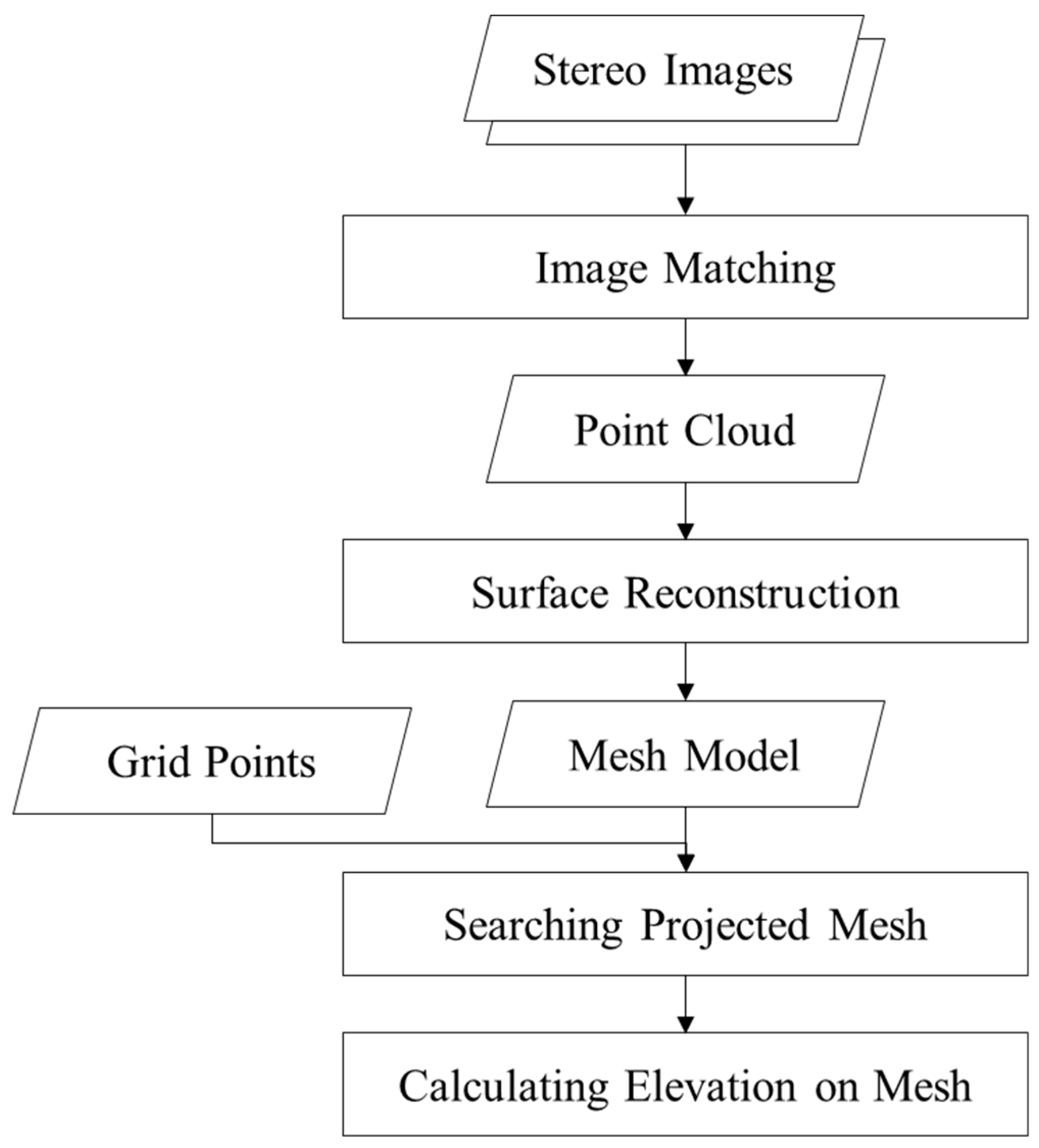
Figure 1 shows the overall work flow of DSM generation from stereo image matching and a 3D mesh model. From stereo images, a point cloud is generated by applying stereo image matching. In this paper, we used the stereo matching algorithms proposed in the work of [4]. A 3D mesh model was then generated from a point cloud created by 3D surface reconstruction. In order to reconstruct a 3D mesh model with a point cloud, it is necessary to estimate the surface normal vectors of the point cloud. The surface normal estimation process consists of surface normal calculation and surface normal adjustment. For each point, we computed the covariance matrix from the nearest neighbors and performed principal component analysis (PCA).
Figure 2 shows the process of estimating a surface normal vector with PCA. This process searches the points surrounding the selected point and calculates a covariance matrix with the neighboring points using Equation (1). PCA can be done by eigenvalue decomposition of the covariance matrix. Then, three eigenvectors are extracted. The eigenvector with the smallest scalar value is estimated as the surface normal vector. In Equation (1), where is the number of point neighbors considered in the neighborhood of , represents the 3D centroid of the nearest neighbors, is the -th eigenvalue of the covariance matrix, and is the -th eigenvector [21].
The direction of the surface normal extracted through PCA may be inconsistent because it is determined using only the surrounding points [22]. For this reason, the directions of the surface normal vectors are adjusted using sensor position. The process of adjusting the direction of the surface normal vector is shown in Figure 3. First, the surface normal vector of each point and the direction vector towards the sensor position at each point are calculated. Then, if the relation between the surface normal vector and the direction vector does not satisfy Equation (2), the direction of the surface normal vector is reversed toward the sensor position. In Equation (2), is the normal vector of , is the sensor position, and represents the position of each point. The sensor position of each point is obtained during extraction of the point cloud by image matching.
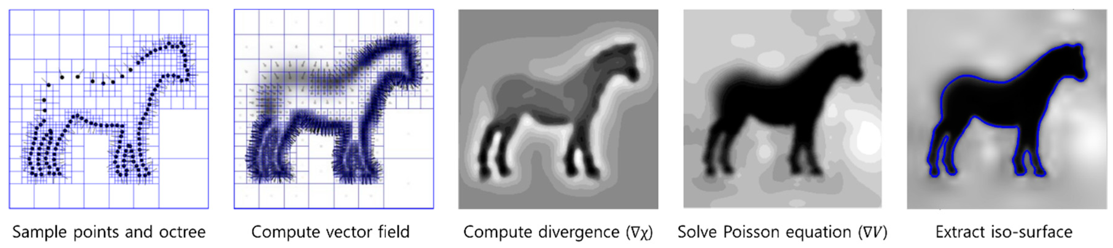
A Poisson surface reconstruction method is then applied to generate a mesh model [23]. This surface reconstruction technique is mainly used to create meshes with unstructured point clouds. As this technique generates a mesh model by estimating the surface using the surface normal of input points, an accurate surface normal is required. This has the advantages of being flexible to noisy data and constructing the surface in a large hole with an empty point [19]. The result produced from the Poisson surface reconstruction method is a smooth approximate surface, positioned near the initial point cloud. An important characteristic of Poisson surface reconstruction is the tendency to over-smooth the data. This may be undesirable in most cases, but it can be adjusted to the current needs of each implementation by defining the depth of the octree. The form of the Poisson surface reconstruction is based on the normal field (inward pointing), which represents the boundary of a solid and may be interpreted as the gradient of the solid’s indicator function. Thus, the main phases of Poisson surface reconstruction of a set of oriented points may be defined as follows: (a) transformation of the oriented point cloud into a continuous vector field in 3D, (b) finding a scalar function whose gradients best match the vector field, and (c) extraction of the appropriate iso-surface. In the next phase, an oriented point cloud is created by resampling the iso-surface. Then, the mesh model is generated using the oriented point cloud.
The surface reconstruction method starts by computing a 3D indicator function, χ, defined as 1 at points inside the model, and as 0 at points outside it (Figure 4). The gradient of the indicator function is non-zero only at points near the surface. At such points, it is taken to be equal to the inward surface normal. Thus, the oriented point samples can be viewed as samples of the gradient of the model’s indicator function. The problem reduces to finding χ where the gradient best approximates vector field V, defined by the input points. Next, if we apply the divergence operator, this problem transforms into a standard Poisson problem. In Equation (4), scalar function χ is calculated, where the Laplacian equals the divergence of vector field V. The implicit function χ is represented using an adaptive octree, rather than a regular 3D grid. The output scalar function χ, represented in an adaptive octree, is then iso-contoured using adaptive marching cubes to obtain the mesh [19]. Figure 5 shows an example of Poisson surface reconstruction in 2D.
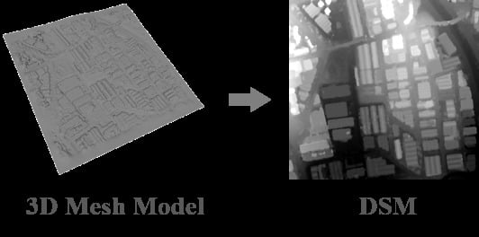
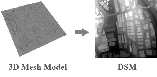
After a 3D mesh model is generated, a DSM is generated with a DSM interpolation process. Figure 6 shows the process of calculating the elevation of a grid point projected onto the mesh. First, grid points are created on the XY plane to generate a DSM. The point spacing of the grid points is determined by the ground sampling distance (GSD) of the DSM to be generated. Then, each grid point searches a vertically projected mesh, and we extract the Z value of the mesh. For this, a plane equation is constructed using the vertex coordinates of a triangular mesh. An elevation value is calculated using the X and Y coordinates of the grid point. If there are several projected meshes, the Z value of the mesh at the highest position is selected as the elevation value of the grid point. Finally, the extracted Z value is set as the elevation value of the grid point, and thereby, the mesh-based DSM is generated [19].
For comparison, we generated interpolations based on a DSM with the IDW method. The IDW method estimates unknown values by specifying search distance, closest points, and the power setting. Formally, the unknown value, ŷ(S0), in location S0, is estimated using the observed y values at sampled locations Si in the following manner:
Essentially, the estimated value in S0 is a linear combination of the weights (λi) and observed y values in Si, where λi is often defined as follows:
In Equation (6), the numerator is the inverse of the distance (d0i) between S0 and Si with a power, α, and the denominator is the sum of all inverse distance weights for all locations i so that the sum of all λi’s for an unsampled point will be 1, as seen in Equation (7). The α parameter is specified as a geometric form for the weight, and it is possible to set other specifications. This specification implies that if α is larger than 1, the distance decay effect will be more than proportional to an increase in distance, and vice versa. Thus, a small α tends to yield estimated values as averages of Si in the neighborhood, whereas a large α tends to give larger weights to the nearest points and increasingly down-weights the points that are farther away [24].
The interpolation-based DSM was created by adjusting the search distance to analyze the tendency to interpolate empty grid cells and the accuracy of the DSM. The unit of the distance is the GSD of the DSM, and means one grid space of the grid data.
2.2. Dataset
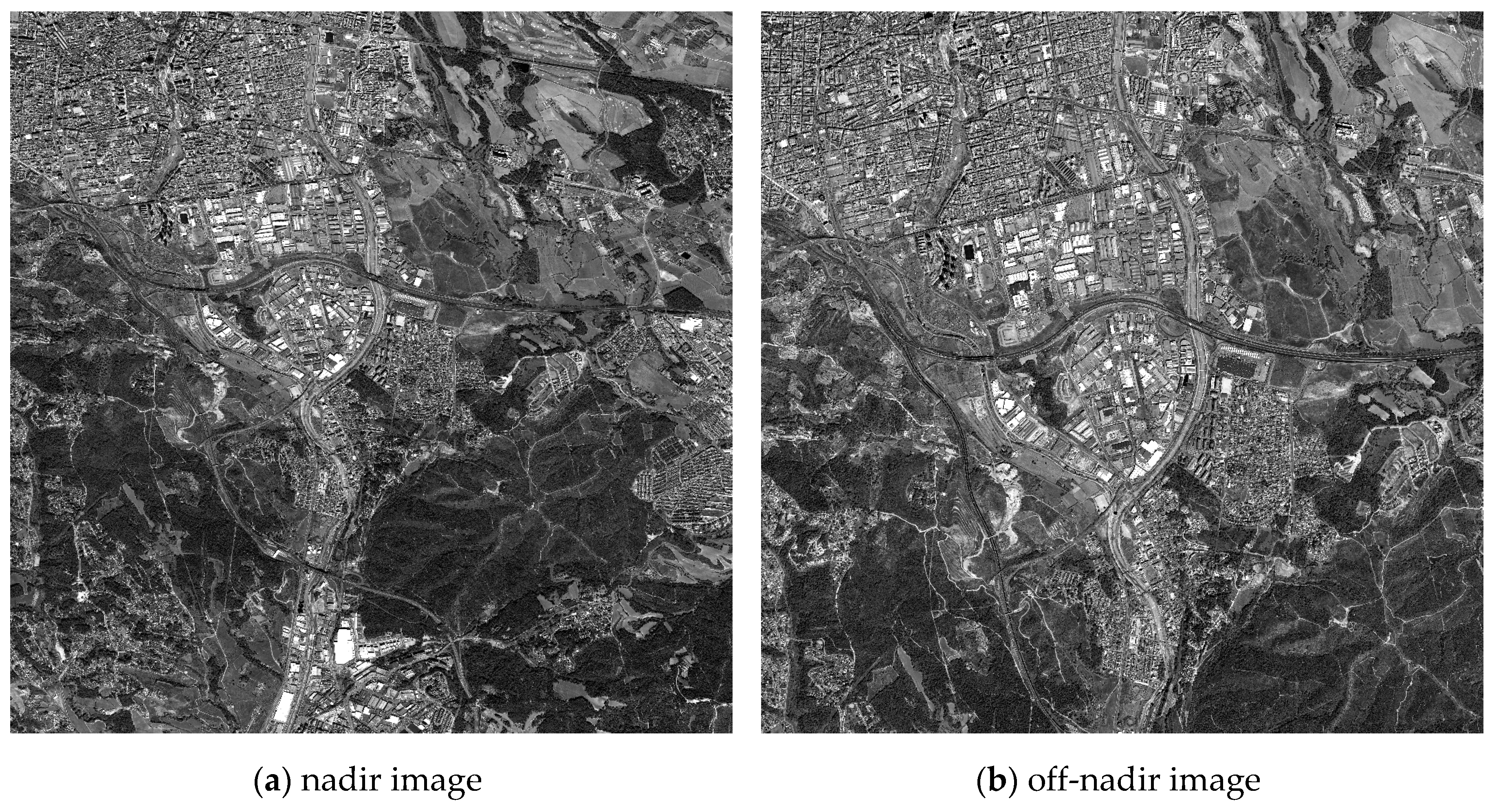
The stereo Worldview-1 images used came from one L1B stereo scene acquired in August 2008. One image was a nadir image (−1.3°), and the other was an off-nadir (33.9°); ground sample distances were 0.5 m and 0.76 m, respectively. Figure 7a is the left image of the stereo pair, and Figure 7b is the right image. The two images were the same size: 10,000 × 10,000 pixels. However, the scale of the two images was not the same as a result of different GSDs.
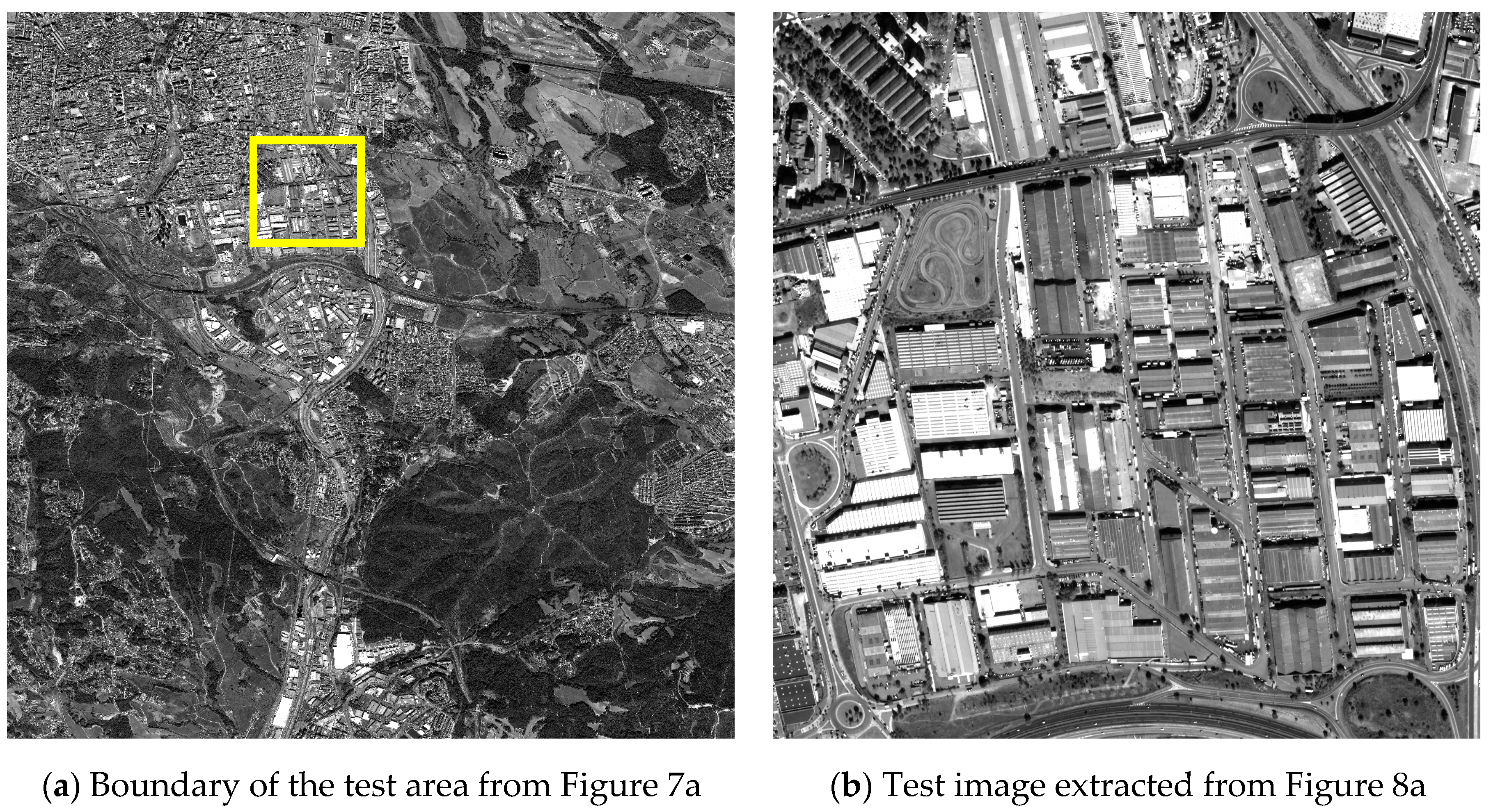
We set up test areas in the original images, and created a point cloud for the test area. The test area was set to about 1 km × 1 km in an urban area of the original stereo images. Figure 8a shows the boundary of the test area in the original left image. Figure 8b is the test image extracted from the original (left) image.
We created the point cloud by applying a stereo image-matching method to the test images. The method performs patch-based image matching using epipolar geometry constraints. Thus, we generated epipolar images through the geometry of the original image. Then, we set epipolar lines to the search range and performed image matching using a search window.
In the image matching process, we used a multi-dimensional search window-based image matching technique [4]. This technique creates a multi-dimensional search window by setting an adaptive and variable search window for the calculation of similarity. The multi-dimensional search window consisted of many sets of full, upper left, upper right, lower left, and lower right windows according to various window sizes. Compared with a fixed window, many similarity comparisons can be performed. It has been reported that this technique presents a more reliable and accurate image matching performance than using a fixed search window when the amount of texture information in the patch and the resolution of the images is different [4]. Figure 9 is an example of a search window set to perform a point match. As can be seen from the figure, a plurality of correlation results is calculated at one target point existing on the epipolar line.
Figure 10 shows a point cloud extracted only for the test area by stereo image matching. The point cloud was generated by matching on a pixel-by-pixel basis using original scale images. Average spacing is 0.7 m. The textured areas in the figure are where the point cloud was generated and textureless areas are where there were no matching results. For example, points on the walls of the building in the test image have been extracted with difficulty because of the usage of one nadir and one off-nadir image. These areas appeared without texture in the right-hand images of Figure 10. There were outlier points and large holes in the point cloud as a result of match failure.
3. Results and Discussion
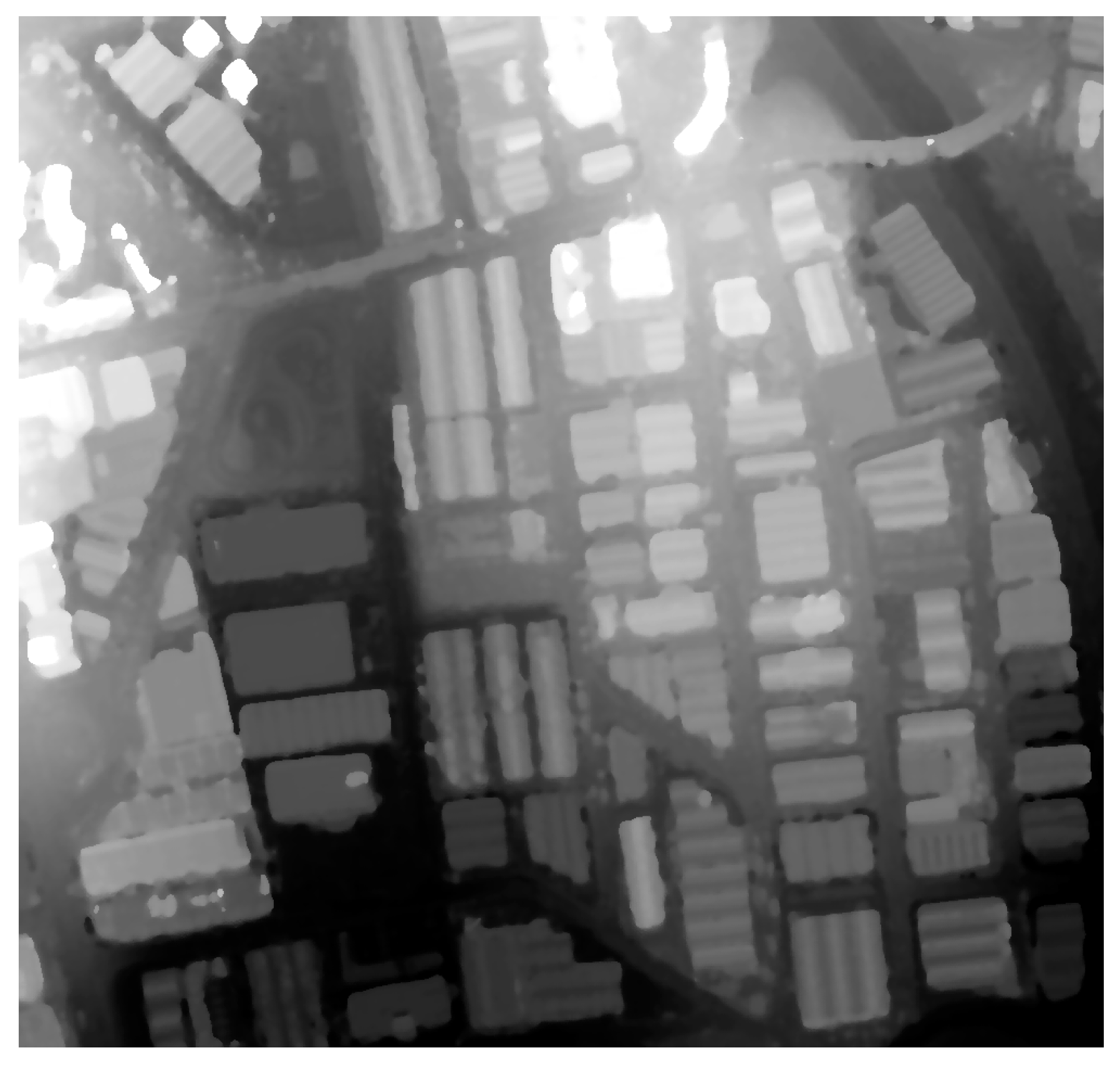
A 3D mesh model was generated from the point cloud using PCA and a Poisson surface reconstruction method to create a mesh-based DSM. In the process of Poisson surface reconstruction, the octree depth level was set to 9, and other parameters were set to default values. We implemented this process through Point Cloud Library 1.8.0 and Microsoft Visual Studio 2013 C++. A 3D mesh model was generated with the point cloud (Figure 11). There were no holes in the mesh model. Then, we created a mesh-based DSM using the proposed method (Figure 12). The GSD of the mesh-based DSM was set to 1 m. There were no empty grid cells and outliers.
For comparing the performance of the mesh-based DSM, we generated an IDW-based DSM using Equations (5)–(7). Parameter was set to 2.
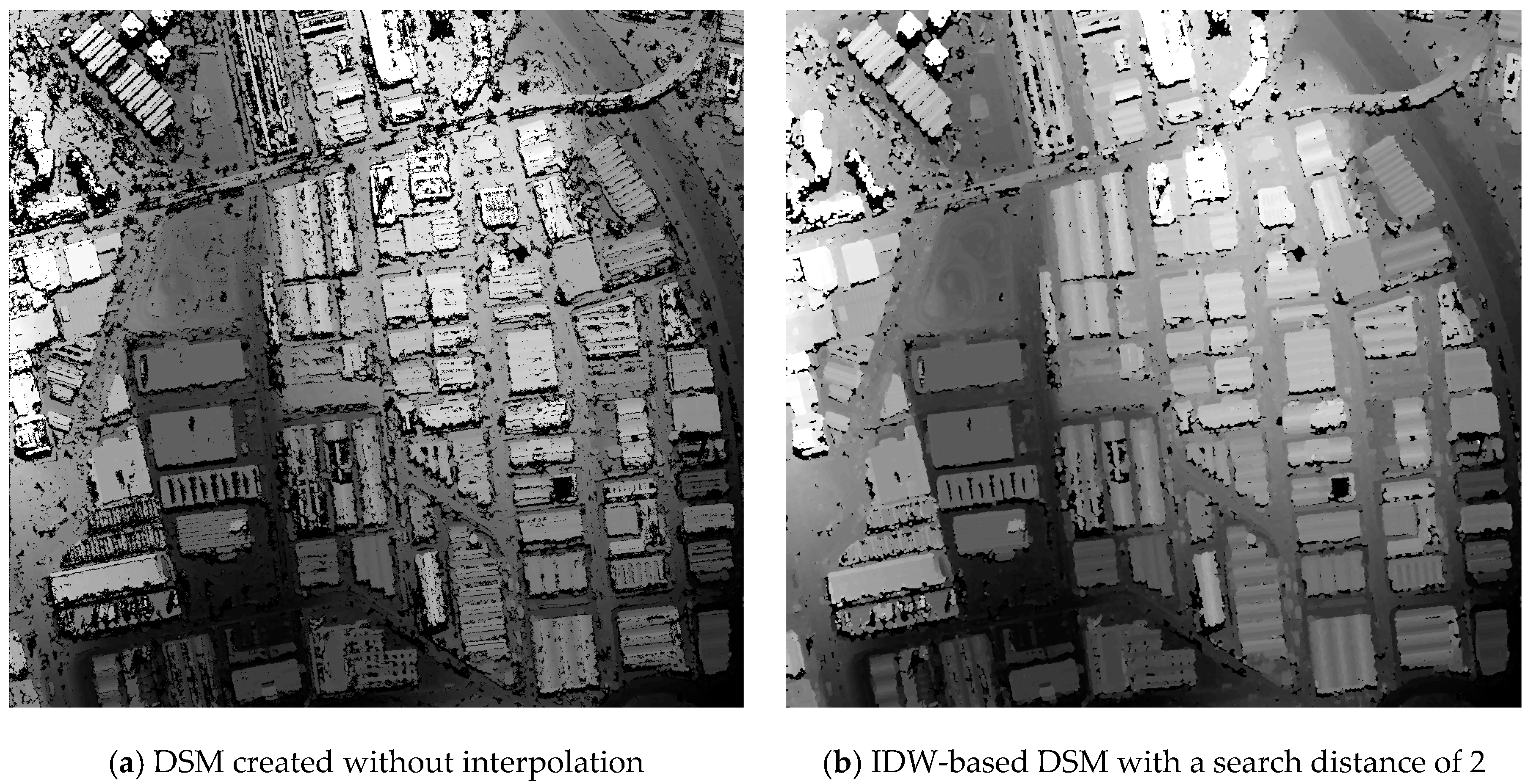
We created the IDW-based DSM repeatedly by increasing the search distance incrementally by one GSD until all empty grids were filled. Figure 13 shows the DSM without interpolation and the IDW-based DSM without empty grid cells. All empty grid cells were interpolated when the search distance was set to 15. For the purpose of conciseness, only the results from search distances of 0, 1, 2, 5, and 15 times GSD are shown.
Table 1 shows the number of empty grid cells and the accuracy of the DSM based on the search distance. The accuracy of the DSM was analyzed with a reference DSM. In this result, we confirmed that the empty grid cells decrease as the search distance increases; however, the accuracy of the DSM gets lower. Moreover, the DSM where all empty grid cells were interpolated by setting the search distance to a large value still had problems with outliers.
As a result, we confirmed that it is difficult to set a search distance to interpolate all empty grid cells. Moreover, we found the search distance where all empty grids were interpolated through the experiment, but error cells generated by outliers were not completely removed.
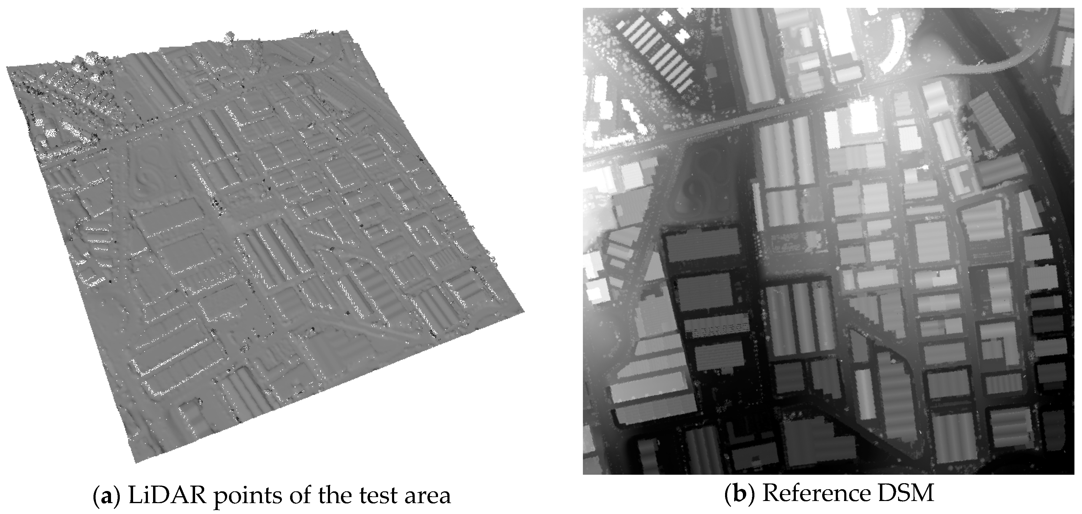
For analyzing the accuracy of DSMs, we generated a reference DSM. The reference data consisted of an airborne laser scanning point cloud (first pulse and last pulse) with approximately 0.3 points per square meter. The LiDAR points were acquired at the end of November 2007. The reference DSM was used to evaluate the accuracy of the DSMs and to generate the ground control point (GCP). GCPs were used to correct the rational rational polynomial coefficient (RPC) parameters of the stereo image.
The reference DSM was created by extracting points from the test area of LiDAR points. The GSD of the reference DSM was set to 1 m, and the elevation of each grid was calculated as the average value. The GSD and geometry information of the DSM generated during the experiment were set to be identical to those of the reference DSM. Figure 14 shows the LiDAR points of the test area, and the reference DSM created with the extracted point cloud.
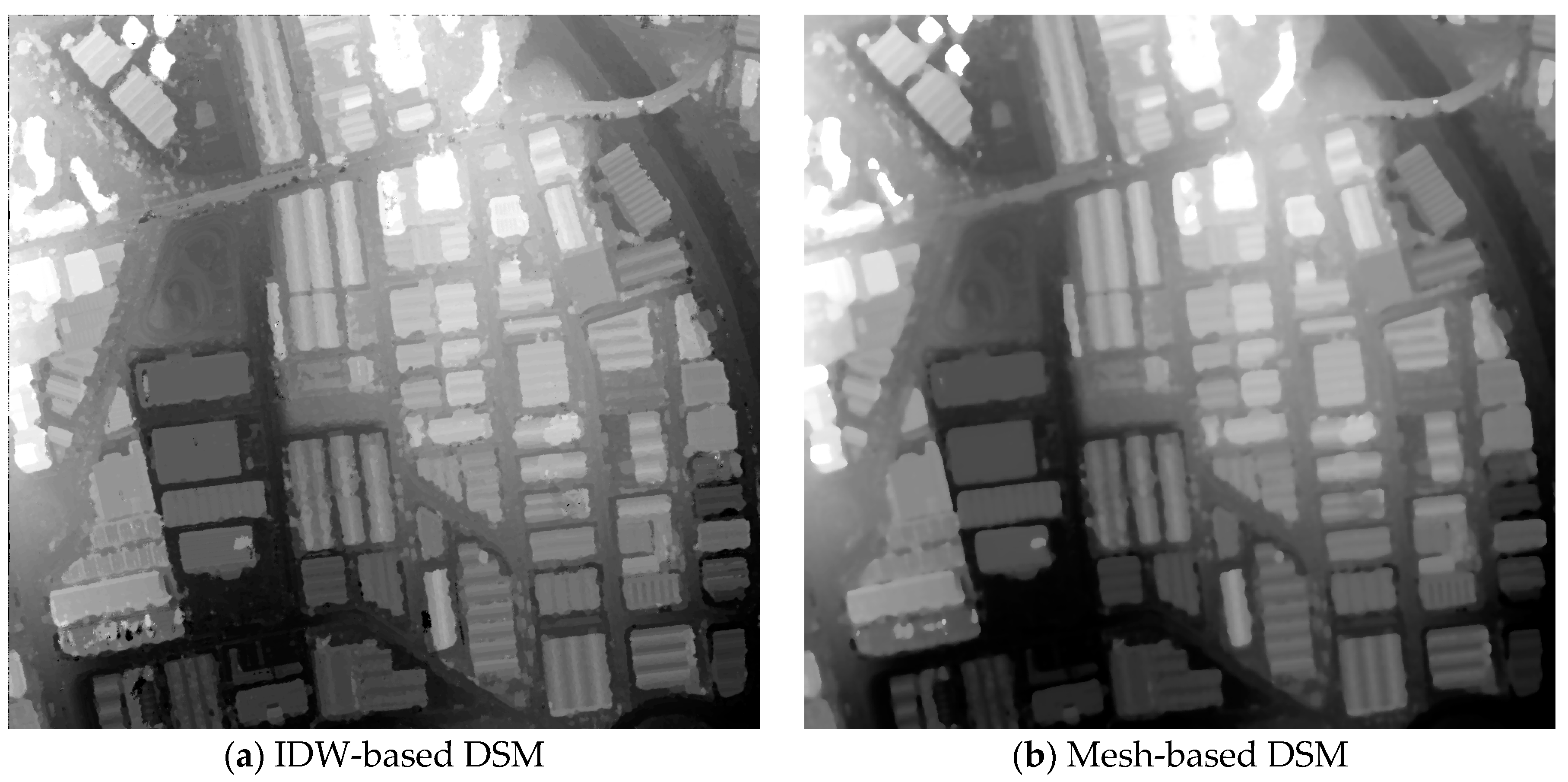
Accuracy was analyzed by calculating the RMSE of the DSMs generated compared with the reference DSM. For additional comparison of DSM quality, we performed a visual analysis to check the clarity of object boundaries of the buildings. Figure 15 shows the results from comparing an IDW-based DSM and a mesh-based DSM. The RMSE of the mesh-based DSM was 2.7983 m, which was better than the accuracy of the interpolation-based DSM with a radius of 15 in Table 1. Figure 15a is the IDW-based DSM and (b) is the mesh-based DSM. Comparing Figure 15a1,b1 shows that because of the nature of surface reconstruction based on mesh models, building boundaries appear smoother on the mesh-based DSM. In the comparison of Figure 15a2,b2, the results show that the problem of a blurred building boundary makes it difficult to differentiate the boundary of the nearest buildings. The red circle in Figure 15b3 means the mesh-based DSM is robust to outliers. As a result, the accuracy of the mesh-based DSM was the best, but the building boundaries were not clear.
Therefore, we performed an additional experiment to create an integrated DSM by combining the IDW-based DSM and the mesh-based DSM. For the experiment, we used an IDW-based DSM with a search distance of 2. The DSM integration processing consisted of replacing the empty cells and filtering outliers of the IDW-based DSM using the mesh-based DSM. In the process of replacing the empty cells, the elevation value of an empty cell in the IDW-based DSM was replaced with the value from the cell in the same position in the mesh-based DSM. In order to interpolate empty grid cells using the mesh-based DSM, it is necessary to extract empty grid cells in the interpolated DSM and find the cell at the same position in the mesh-based DSM. Therefore, the GSD of the two DSMs should be set to the same value. In this experiment, we set GSD to 1.0 m because the GSD of the reference data was set to 1.0 m. In the process of replacing empty grid cells, outliers in the interpolation-based DSM were not replaced. These outliers degrade the quality of the integrated DSM. On the other hand, the mesh-based DSM is robust to noise such as outliers. Therefore, if the elevation difference between the mesh-based DSM and the interpolation-based DSM in a cell at the same position is large, the elevation of the interpolation-based DSM is likely to be the outlier. In the DSM integration step, if the elevation difference between each DSM is greater than a set threshold, we defined the elevation as the outlier and replaced it with the elevation of the mesh-based DSM. In this experiment, the threshold to remove an outlier was set at 3 m.
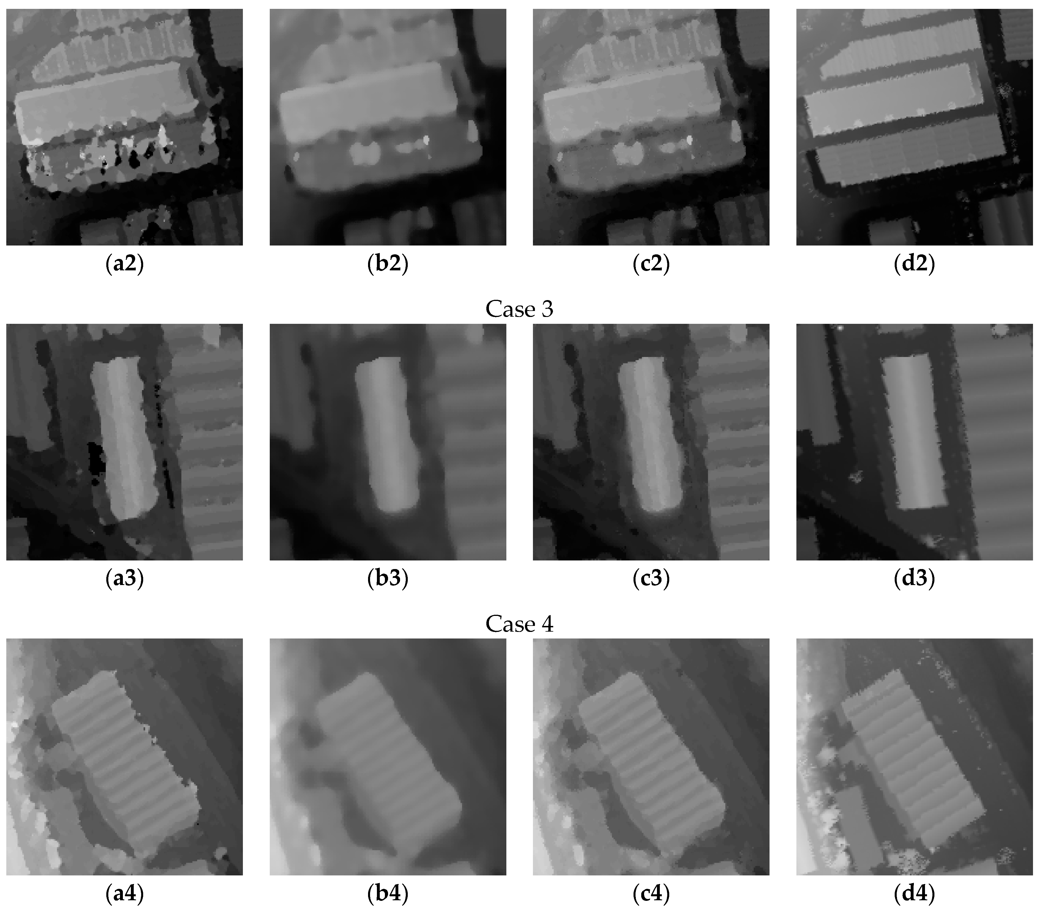
Figure 16 shows the IDW-based DSM, the mesh-based DSM, the integrated DSM, and the reference DSM. Figure 16a shows the IDW-based DSM without empty grid cells. Figure 16c is the integrated DSM created by setting the search distance of the IDW interpolation to 2. When set to 1, the integrated DSM was less affected by large holes, and the building boundaries were clear. For settings of 2, 3, and 4, the clarity of the boundary of the buildings was maintained, and most of the error cells due to outliers were removed. In particular, the result of the comparison between Figure 16a4,c4 shows that much noise disappeared from the building boundaries.
Table 2 shows the accuracy of DSMs created by different interpolation methods. The accuracy of the integrated DSM was better than that of the IDW-based DSM and lower than that of the mesh-based DSM.
As mentioned before, IDW has limitations in interpolating the DSM of an urban area because of outliers and large holes in the point cloud created from stereo image matching. The results of the comparison showed that the mesh-based DSM has successfully improved the problem of outliers and holes. However, the mesh-based DSM also has the limitation of blurring the building boundaries. We suspect that this side effect was caused from over-smoothing in the surface reconstruction method [25]. The results of the comparison between the integrated DSM and other DSMs (Figure 16 and Table 2) showed that our proposed method can improve the accuracy and maintain the sharpness of object boundaries.
Unlike previous studies using the auxiliary DSM, our results showed that interpolation method using the mesh model can be a good candidate for generating the DSM from stereo image matching when there is no knowledge of surface type or supplementary data available. Moreover, in the relevant study [9], they used only the original images and the unfilled DSM itself for interpolation. Their proposed method utilizes the shadow information and image segmentation information from the original images. They conducted DSM interpolation experiments on high-resolution satellite images of urban areas and reported an accuracy of 3.3 m. Thus, we expect that our proposed method with additional information extracted from the original images can improve DSM interpolation performance.
4. Conclusions
This paper proposed a new DSM interpolation method based on a 3D mesh model to handle outliers and large holes more efficiently without any a priori knowledge of surface types. We showed that the surface reconstruction method, which has been used mainly for 3D visualization, could be used for DSM interpolation as an alternative solution to interpolation models based on a local distribution model. In the results of the experiments, the mesh-based DSM was more accurate than the IDW-based DSM, and there were no erroneous grid cells due to large holes and outliers. However, object boundaries were smoothed out on the mesh-based DSM owing to the nature of surface reconstruction techniques. To overcome this weakness, we integrated the two DSMs to fill the erroneous grid cells and maintain the clarity of the boundaries. We confirmed that DSM quality was improved by the integration.
From this paper, it will be possible to complement the limits of the previous interpolation method. In particular, the proposed method is expected to contribute to improving the quality of a DSM that is generated by images of urban areas with large artificial structures. In the future, we will perform experiments to segment areas in an image domain and interpolate areas that are semantically classified. The limitations of our experiments include having processed an area that is mostly urban. Although we chose this type because it is the most challenging, we need to test the proposed method with various surface types. Our future research will include an extension of the proposed method to apply it to the generation of digital terrain models where non-terrain objects have to be removed and replaced by interpolation of neighboring terrain heights.
Author Contributions
Research design and supervision by T.K.; Methodology, S.K.; Literature review and discussion S.K., T.K. and S.R.; Software, S.K.; Validation, S.K. and T.K.; Formal analysis, S.K.; Data processing and analysis, S.K. and S.R.; Writing (original draft reparation), S.K.; Writing (review and editing), S.K. and T.K.; Funding acquisition, S.R.; Project administration, S.R.
Funding
This research was supported by a grant (18SIUE-B148326-01) from CAS 500-1/2 Image Acquisition and Utilization Technology Development funded by the Ministry of Land, Infrastructure, and Transport (MOLIT) of the Korea government and the Korea Agency for Infrastructure Technology Advancement (KAIA).
Conflicts of Interest
The authors declare no conflict of interest.
References
- Wang, L.; Neumann, U. A robust approach for automatic registration of aerial images with untextured aerial LiDAR data. In Proceedings of the IEEE Conference on Computer Vision and Pattern Recognition 2009, Miami, FL, USA, 20–25 June 2009; pp. 2623–2630. [Google Scholar]
- Hirschmller, H. Stereo Processing by Semiglobal Matching and Mutual Information. IEEE Trans. Pattern Anal. Mach. Intell. 2008, 30, 328–341. [Google Scholar] [CrossRef] [PubMed] [Green Version]
- Lee, H.Y.; Kim, T.; Park, W.; Lee, H.K. Extraction of digital elevation models from satellite stereo images through stereo matching based on epipolarity and scene geometry. Image Vis. Comput. 2003, 21, 789–796. [Google Scholar] [CrossRef]
- Rhee, S.; Kim, T. Dense 3D Point Cloud Generation from UAV Images from Image Matching and Global Optimazation. Remote Sens. Spat. Inf. Sci. 2016, 41, 1005–1009. [Google Scholar]
- Choi, H.; Hong, S. Utilization Methods and Generation DEMs by Using Aerial Photographs. J. Korea Contents Assoc. 2007, 7, 168–175. [Google Scholar] [CrossRef] [Green Version]
- Setianto, A.; Triandini, T. Comparison of kriging and inverse distance (IDW) interpolation methods in lineament extraction and analysis. J. Appl. Geol. 2013, 5, 21–29. [Google Scholar]
- Lloyd, C.D.; Atkinson, P.M. Deriving DSMs from LiDAR data with kriging. Int. J. Remote Sens. 2002, 23, 2519–2524. [Google Scholar] [CrossRef]
- Gonçalves, G. Analysis of interpolation errors in urban digital surface models created from Lidar data. In Proceedings of the 7th International Symposium on Spatial Accuracy Assessment in Natural Resources and Environmental Sciences, Lisbon, Portugal, 5–7 July 2006. [Google Scholar]
- Bafghi, Z.G.; Tian, J.; Angelo, P.; Reinartz, P. A new algorithm for void filling in a DSM from stereo satellite images in urban areas. ISPRS Ann. Photogramm. Remote Sens. Spat. Inf. Sci. 2016, 3, 55–61. [Google Scholar] [CrossRef]
- Grohman, G.; Kroenung, G.; Strebeck, J. Filling SRTM voids: The delta surface fill method. Photogramm. Eng. Remote Sens. 2006, 72, 213–216. [Google Scholar]
- Karkee, M.; Kusanagi, M.; Steward, B.L. Fusion of Optical and InSAR DEMs: Improving the Quality of Free Data. In Proceedings of the 2006 ASABE Annual International Meeting, Portland, OR, USA, 9–12 July 2006; Volume 43, p. 1. [Google Scholar]
- Ling, F.; Zhang, Q.W.; Wang, C. Filling voids of SRTM with Landsat sensor imagery in rugged terrain. Int. J. Remote Sens. 2007, 28, 465–471. [Google Scholar] [CrossRef]
- Yue, T.X.; Chen, C.F.; Li, B.L. A high-accuracy method for filling voids and its verification. Int. J. Remote Sens. 2012, 33, 2815–2830. [Google Scholar] [CrossRef]
- Grimaldi, S.; Teles, V.; Bras, R.L. Sensitivity of a physically based method for terrain interpolation to initial conditions and its conditioning on stream location. Earth Surf. Process. Landf. 2004, 29, 587–597. [Google Scholar] [CrossRef]
- Grimaldi, S.; Teles, V.; Bras, R.L. Preserving first and second moments of the slope area relationship during the interpolation of digital elevation models. Adv. Water Resour. 2005, 28, 583–588. [Google Scholar] [CrossRef]
- Dowding, S.; Kuuskivi, T.; Li, X. Void Fill of SRTM Elevation Data—Principles, Processes and Performance. 2004. Available online: http://www.tsym3.selcuk.edu.tr/docs/dowding_etal.pdf (accessed on 31 October 2018).
- Kuuskivi, T.; Lock, J.; Li, X.; Dowding, S.; Mercer, B. Void fill of SRTM elevation data: Performance evaluations. In Proceedings of the ASPRS Annual Conference 2005, Baltimore, MD, USA, 7–11 March 2005; pp. 7–11. [Google Scholar]
- Reuter, H.I.; Nelson, A.; Jarvis, A. An evaluation of void-filling interpolation methods for SRTM data. Int. J. Geogr. Inf. Sci. 2007, 21, 983–1008. [Google Scholar] [CrossRef]
- Kazhdan, M.; Bolitho, M.; Hoppe, H. Poisson Surface Reconstruction. In Proceedings of the 4th Eurographics Symposium on Geometry Processing, Cagliari, Sardinia, Italy, 26–28 June 2006. [Google Scholar]
- Rusu, R.B.; Marton, Z.C.; Blodow, N.; Beetz, M. Persistent point feature histograms for 3D point clouds. Auton. Syst. 2008, 10, 119–129. [Google Scholar]
- Smith, L.I. A Tutorial on Principal Components Analysis; Cornell University: Ithaca, NY, USA, 2002; Volume 51, pp. 12–17. [Google Scholar]
- Hoppe, H.; DeRose, T.; Duchamp, T.; McDonald, J.; Stuetzle, W. Surface reconstruction from unorganized points. In Proceedings of the 19th Annual Conference on Computer Graphics and Interactive Techniques, Chicago, IL, USA, 27–31 July 1992; pp. 71–78. [Google Scholar]
- Kazhdan, M.; Hoppe, H. Screened Poisson surface reconstruction. ACM Trans. Graph. 2013, 32, 29. [Google Scholar] [CrossRef]
- Lu, G.Y.; Wong, D.W. An adaptive inverse-distance weighting spatial interpolation technique. Comput. Geosci. 2008, 34, 1044–1055. [Google Scholar] [CrossRef]
- Hornung, A.; Kobbelt, L. Robust reconstruction of watertight 3D models from non-uniformly sampled point clouds without normal information. In Proceedings of the Fourth Eurographics Symposium on Geometry Processing 2006, Cagliari, Sardinia, Italy, 26–28 June 2006; pp. 41–50. [Google Scholar]
Figure 1.
Workflow for generating a mesh-based digital surface model (DSM).

Figure 2.
Estimating a surface normal vector with principal component analysis (PCA).

Figure 3.
Adjusting the surface normal based on the geometry condition with a sensor position vector.
Figure 3.
Adjusting the surface normal based on the geometry condition with a sensor position vector.

Figure 4.
Concept of Poisson surface reconstruction in 2D.

Figure 5.
Example of Poisson surface reconstruction in 2D.

Figure 6.
Process of extracting the elevation of grid points from a mesh model.

Figure 7.
Stereo Worldview-1 images from August 2008.

Figure 8.
Stereo Worldview-1 images.

Figure 9.
Multi-dimensional search window (five steps).

Figure 10.
Point cloud of the test area.

Figure 11.
3D mesh model of the test area.

Figure 12.
Mesh-based DSM.

Figure 13.
DSMs according to increasing search distances. IDW—inverse distance weight.


Figure 14.
Reference data. LiDAR—light detection and ranging.

Figure 15.
Comparison results of DSMs created with IDW and mesh. (a1) building boundary of the IDW-based DSM, (b1) building boundary of the mesh-based DSM, (a2) separated boundaries of buildings of the IDW-based DSM, (b2) blurry boundaries of buildings of the mesh-based DSM, (a3) noise of the IDW-based DSM, (b3) interpolated surface of the mesh-based DSM.


Figure 16.
Comparison of the resulting DSMs. (a1–a4) results from the IDW-based DSM, (b1–b4) results from the mesh-based DSM, (c1–c4) results from the integrated DSM, (d1–d4) results from the reference DSM.
Figure 16.
Comparison of the resulting DSMs. (a1–a4) results from the IDW-based DSM, (b1–b4) results from the mesh-based DSM, (c1–c4) results from the integrated DSM, (d1–d4) results from the reference DSM.


Table 1.
The accuracy of the inverse distance weight (IDW)-based digital surface model (DSM) with search distance adjustment. GSD—ground sampling distance; RMSE—root mean square error.
Table 1.
The accuracy of the inverse distance weight (IDW)-based digital surface model (DSM) with search distance adjustment. GSD—ground sampling distance; RMSE—root mean square error.
| Search Distance (Unit GSD) | 0 | 1 | 2 | 5 | 15 |
|---|---|---|---|---|---|
| Number of all cells | 950,000 | ||||
| Number of empty grid cells | 229,851 (24%) | 183,940 (19%) | 68,208 (7%) | 6,686 (1%) | 0 (0%) |
| RMSE of all cells (m) | 2.3840 | 2.4661 | 2.8084 | 3.1537 | 3.2160 |
Table 2.
Comparison of the accuracy of the DSMs.
| Interpolation Method | IDW | Mesh | Integration |
|---|---|---|---|
| RMSE (m) | 3.2160 | 2.7983 | 2.9104 |
© 2018 by the authors. Licensee MDPI, Basel, Switzerland. This article is an open access article distributed under the terms and conditions of the Creative Commons Attribution (CC BY) license (http://creativecommons.org/licenses/by/4.0/).
Share and Cite
MDPI and ACS Style
Kim, S.; Rhee, S.; Kim, T. Digital Surface Model Interpolation Based on 3D Mesh Models. Remote Sens. 2019, 11, 24. https://doi.org/10.3390/rs11010024
AMA Style
Kim S, Rhee S, Kim T. Digital Surface Model Interpolation Based on 3D Mesh Models. Remote Sensing. 2019; 11(1):24. https://doi.org/10.3390/rs11010024
Chicago/Turabian StyleKim, Soohyeon, Sooahm Rhee, and Taejung Kim. 2019. "Digital Surface Model Interpolation Based on 3D Mesh Models" Remote Sensing 11, no. 1: 24. https://doi.org/10.3390/rs11010024
Note that from the first issue of 2016, this journal uses article numbers instead of page numbers. See further details here.