Exploring Bamboo Forest Aboveground Biomass Estimation Using Sentinel-2 Data

Abstract

Bamboo forests, due to rapid growth and short harvest rotation, play an important role in carbon cycling and local economic development. Accurate estimation of bamboo forest aboveground biomass (AGB) has garnered increasing attention during the past two decades. However, remote sensing-based AGB estimation for bamboo forests is challenging due to poor understanding of the mechanisms between bamboo forest growth characteristics and remote sensing data. The objective of this research is to examine the remote sensing characteristics of on-year and off-year bamboo forests at different dates and their AGB estimation performance. This research used multiple Sentinel-2 data to explore AGB estimation of bamboo forests in Zhejiang Province, China, by taking into account the unique characteristics of on-year and off-year bamboo forest growth features. Combining field survey data and Sentinel-2 spectral responses (spectral bands and vegetation indices) and textural images, random forest was used to identify key variables for AGB estimation. The results show that (1) the on-year and off-year bamboo forests have considerably different spectral signatures, especially in the wavelengths between red edge 2 and near-infrared wavelength (NIR2) (740–865 nm), making it possible to separate on-year and off-year bamboo forests; (2) on-year bamboo forests have similar spectral signatures although AGB increases from as small as 40 Mgha⁻¹ to as high as 90 Mgha⁻¹, implying that optical sensor data cannot effectively model on-year bamboo AGB; (3) off-year bamboo AGB has significant relationships with red and shortwave infrared (SWIR) spectral bands in the April image and with red edge 2 in the July image, but the AGB saturation problem yields poor estimation accuracy; (4) stratification considerably improved off-year bamboo AGB estimation but not on-year, non-stratification using the April image is recommended; and (5) Sentinel-2 data cannot solve the bamboo AGB data saturation problem when AGB is greater than 70 Mgha⁻¹, similar to other optical sensor data such as Landsat. More research should be conducted in the future to integrate multiple sources—remotely sensed data (e.g., lidar, optical sensor data) and ancillary data (e.g., soil, topography)—into AGB modeling to improve the estimation. The use of very high spatial resolution images that can effectively extract tree density information may improve bamboo AGB estimation and yield new insights.

1. Introduction

Bamboo forests occur extensively in tropical and subtropical regions, playing important roles in improving economic conditions by providing construction materials and food (bamboo shoots) and influencing carbon cycling due to their unique characteristics of rapid growth and short harvest rotation [1,2,3]. The continuous increase of bamboo forest area in the world and its important role in carbon sequestration make mapping its distribution and modeling aboveground biomass (AGB) urgent tasks [4,5,6,7]. The ability to repeatedly capture land surface features makes remote sensing a major data source for quickly updating spatial distribution of bamboo forests and estimating AGB [1,2,3,8]. However, compared to broadleaf and coniferous forests, bamboo forests have some unique characteristics during growth stages [9] that result in challenges when using remote sensing techniques to model AGB in large areas [10,11].

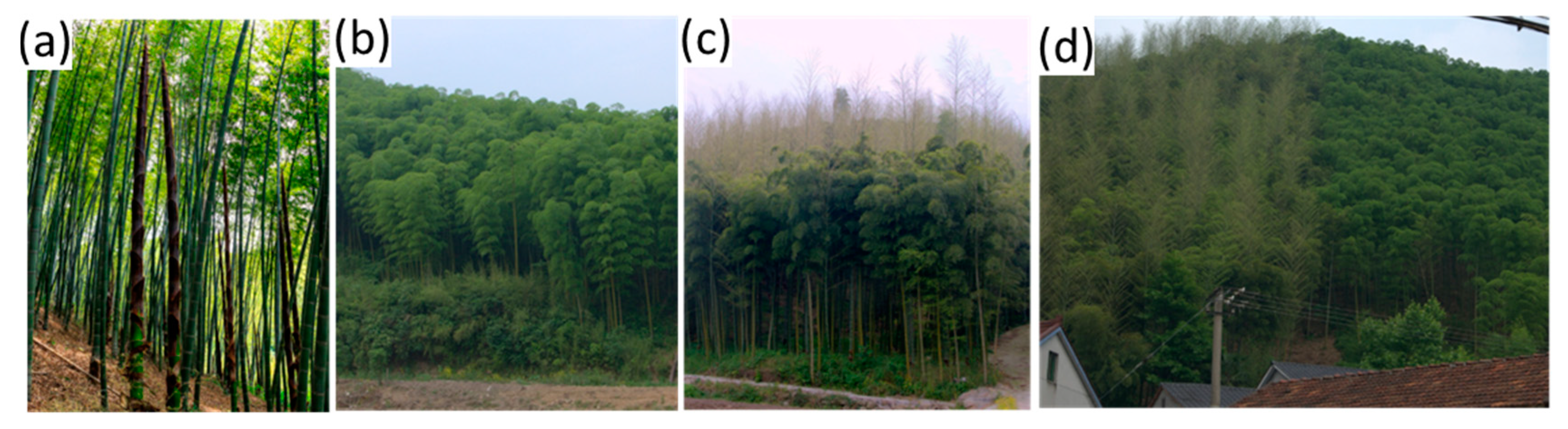
As shown in Figure 1, bamboo forests can change quickly in a short time and have some unique characteristics: (1) On-year and off-year phenomena: An “on-year bamboo forest” represents many bamboo shoots growing during spring (Figure 1a), whereas in an “off-year bamboo forest” almost no bamboo shoots grow (Figure 1b). (2) Rapid growing period of bamboo shoots to fully developed trees (Figure 1c): In the on-year bamboo forest, bamboo shoots emerge between mid-March and mid-April, then take about 40 to 60 days to attain full size (usually until May), depending on soil conditions, and the leaves develop completely in June [9]. (3) Visibility of bamboo canopy: The boundary between on-year and off-year bamboo forest canopy is very clear from April to September (Figure 1d). (4) Intensive management of bamboo forests: In a typical site, forest owners may remove some bamboo shoots in early spring and cut old bamboo trees during fall and early winter; they also remove tree crowns (about 2 to 3 m) of the newly grown bamboo trees in November to make brooms and to avoid tree falls due to snow in the winter. (5) On-year and off-year bamboo forests have different stand structures between April and November but are similar after removal of crowns (Figure 1d), mainly between December and March.

Due to the unique growth stages resulting in a change in stand structure within one year [9], on-year and off-year bamboo forests display different or similar colors on the images, depending on the season (Figure 2). The on-year and off-year bamboo forests in April and May have clear color differences (Figure 2a,b), implying that they can be easily separated, while in July such differences almost disappear (Figure 2c) and they are difficult to distinguish based on spectral signatures. In particular, the difference of on-year and off-year bamboo forests in color composites disappear after summer and before spring seasons (Figure 2d–f). The color changes in the true color composites from Sentinel-2 images at different dates throughout a year imply the importance of selecting suitable image acquisition dates for separation of on-year and off-year bamboo forest distribution and for AGB estimation, which previous research has not explored.

When remote sensing data and sample plots are determined, selection of suitable variables and use of proper modeling algorithms are two critical steps for AGB studies in a given region [12,13]. Many studies have examined the mapping of bamboo forest distribution and modeling AGB using remote sensing data such as Landsat [2,14]. In addition to spectral bands, vegetation indices, image transform algorithms such as principal component analysis (PCA), and textures are often used, and stepwise regression is used to identify the variables for AGB modeling [2,14,15,16]. Meanwhile, radar data such as ALOS (Advanced Land Observing Satellite) PALSAR (Phased Array type L-band Synthetic Aperture Radar) are also used for AGB estimation, but the estimation accuracy is not much better than with Landsat images [11]. Since different remote sensing (e.g., optical, radar, lidar) data with various spectral and spatial resolutions are available, a large number of potential variables may be used [12,17]. However, properly identifying key variables is critical for accurately estimating AGB, and the selected variables may vary considerably depending on the characteristics of forest types under investigation and remotely sensed data itself [10,11,18]. The impacts of forest phenology, growth conditions, and external factors such as moisture on remotely sensed data in representing forest canopy structure make AGB model transfer difficult [19]. Due to the intensive management (e.g., fertilization, selective logging) and the short growth period from bamboo shoots to fully developed bamboo trees [9], remote sensing-based AGB estimation for bamboo forests becomes especially challenging.

In addition to the selection of suitable variables, another critical step is to determine which algorithm should be used for developing the AGB estimation model [12]. Lu et al. [12] summarized the major characteristics of common algorithms used for AGB modeling, including parametric-based algorithms (e.g., regression-based methods) and non-parametric algorithms (e.g., k-nearest neighbor (kNN), artificial neural network (ANN), support vector regression (SVR)). The regression-based modeling approach is often used for developing AGB estimation; in particular, stepwise regression can automatically identify the variables for AGB modeling [13,14]. However, regression-based approaches require the assumption that the selected variables have linear relationships with AGB. In reality, the relationships between AGB and remote sensing-derived variables may be nonlinear, resulting in poor estimation accuracy, for example, the relative root mean squared error can be over 40% [13]. Therefore, in recent years, many studies have explored the use of machine learning algorithms such as kNN, ANN, SVR, and random forest (RF) for bamboo AGB estimation [5,13,20,21]. In particular, RF can provide the importance ranking of the variables [13] and is extensively employed for AGB modeling [22,23,24,25]. RF is a nonparametric ensemble modeling approach that can effectively construct numerous small regression trees for predictions [26]. Compared with other machine learning algorithms such as ANN and kNN, one key advantage of using RF is its ability to provide the importance ranking of the variables. This characteristic is especially valuable when key variables need to be identified from many potential variables. Another advantage is RF’s ability to deal with noise and large datasets [27,28] because it is insensitive to noisy data in training datasets.

In remote sensing-based AGB estimation, one important factor influencing AGB estimation accuracy is the data quality, including ground-truth and remotely sensed data [12]. The dates of sample collection and image acquisition are often inconsistent due to the variable availability of remotely sensed data in frequently cloud-covered tropical and subtropical regions [10,29]. Most previous studies assumed that different dates between sample collection and image acquisition would not significantly influence the relationships between AGB and remote sensing-derived variables [30]. This assumption may be valid for some forest types because forest growth in a short time period will not significantly change the forest stand structure, thus the spectral signature should be similar too. However, this assumption may not be valid for bamboo forests because of the completely different growth stages of bamboo forests (see Figure 1) and broadleaf or coniferous forests [10].

Although studies for modeling bamboo forest AGB have gained increasingly attention, some critical questions remain to be answered. For example, how do different bamboo growth stages affect AGB estimation performance? How do the unique features of on-year and off-year bamboo forests affect AGB estimation? Can the increase of spectral bands in red edge and NIR wavelengths in Sentinel-2 data compared to the common Landsat data improve AGB estimation? In subtropical regions, acquiring cloud-free Landsat images is often difficult due to the cloud-cover problem and relatively low re-visit frequency. The higher spatial and temporal resolutions and more spectral bands in red edge and NIR wavelengths in Sentinel-2 data than in Landsat may provide new insights in bamboo forest AGB studies, but they have not been examined yet.

The overall goals of this research are to explore the impacts of on-year and off-year bamboo forests on AGB modeling effects and the potential role of increased spectral bands in Sentinel-2 data in improving AGB estimation. Specifically, the objectives of this research are to (1) better understand the impacts of on-year and off-year bamboo forests on AGB estimation, (2) understand the impacts of suitable image acquisition dates for AGB estimation, (3) examine AGB saturation in Sentinel-2 data, and (4) better understand the mechanism of bamboo forest AGB estimation using optical sensor data. The new contribution of this research is to better understand the impacts of the unique characteristics of bamboo growing stages on AGB estimation, the impacts of on-year and off-year bamboo forests on AGB estimation, and the roles of multi-seasonal Sentinel-2 images in mapping on-year and off-year bamboo forest distribution and AGB estimation.

2. Materials and Methods

2.1. Study Area

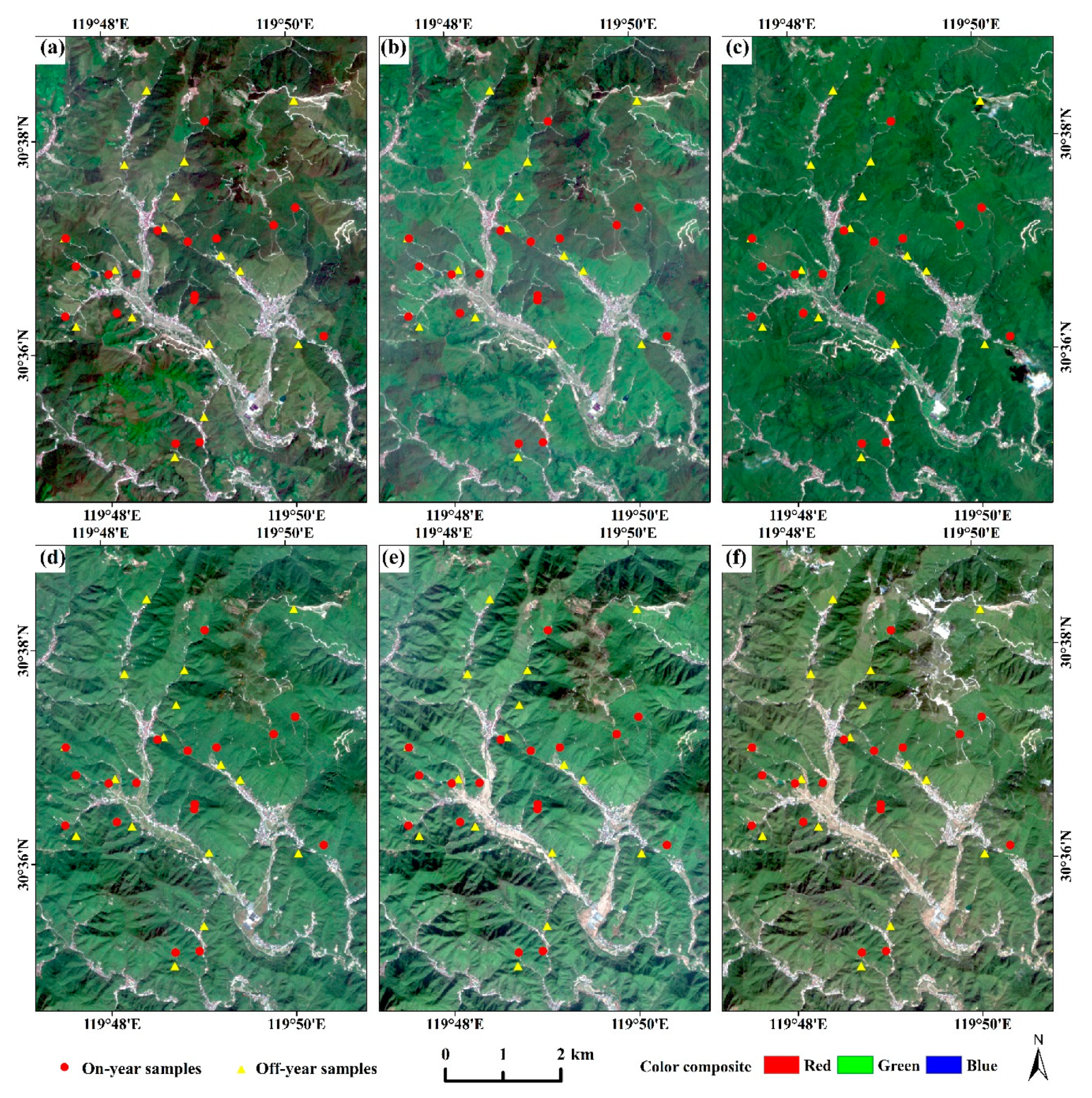
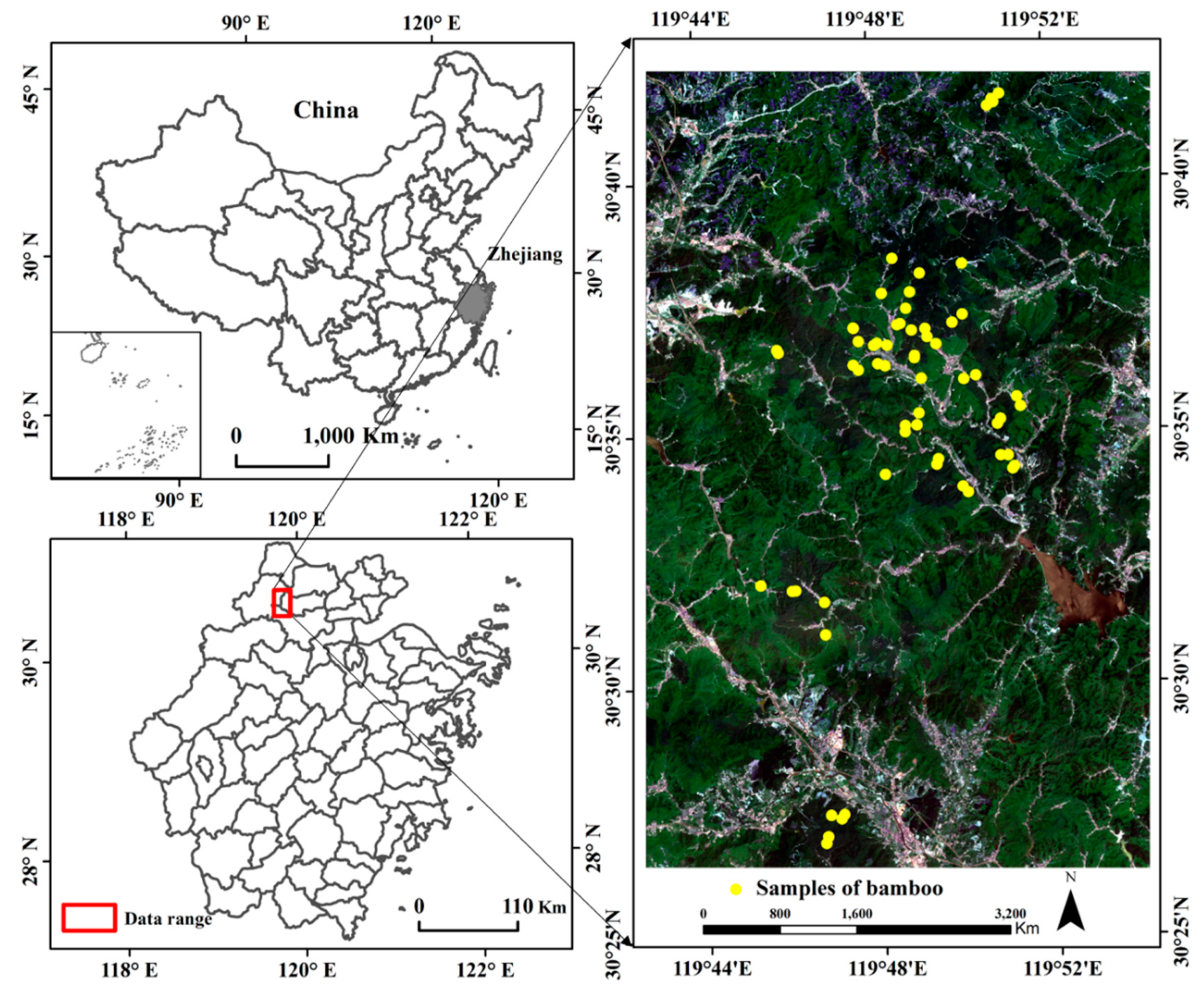
The study area is located in northwest Zhejiang Province, China (Figure 3), covering about 538.06 km². The terrain is undulating with elevations between 20 and 846 m and average slope of 16 degrees. Five soil types—red, yellow, lithologic, fluvoaquic, and paddy—were found [31]. The climate in this region is subtropical monsoon that has abundant illumination and precipitation with four distinct seasons: Warm in spring, hot and humid in summer, cool in fall, cold and damp in winter. The average annual temperature is 15 °C with the lowest temperature of 2 °C in winter and the highest temperature of 37 °C in summer. Annual rainfall is 1400 mm with the highest rainfall in June and lowest rainfall in December [32].

This study area is in subtropical evergreen forests, including coniferous evergreen, broadleaf evergreen, and bamboo. There are also other plantations such as pines, Chinese fir, and agroforestry. Moso bamboo forest (Phyllostachys pubescens) is the most widely distributed bamboo forest type in this study area, accounting for 86% of the total bamboo forests [31]. Moso bamboo trees are taller and have larger diameter at breast height (DBH) than any other bamboo forests such as Phyllostachy snuda [32]. The average height of Moso bamboo is between 9 and 12 m and the average DBH is between 8 and 11 cm. In addition, Moso bamboo forests have single species and stand structure, but stand densities may vary greatly in sites and different seasons because of their on-year and off-year growth characteristics and intensive management, such as selective logging of trees 3 du or older in the on-year bamboo forests during winter [33].

2.2. Data Preparation

The datasets used in our research are summarized in

Table 1. Data used in research.

Data	Description
Field survey	1. A total of 517 sample plots covering different land-cover types were collected in 2016 to 2018. Of these sample plots, about 300 were bamboo forests, including on-year and off-year. 2. A total of 62 sample plots, including 31 on-year and 31 off-year, with plot size of 400 m2 each, were inventoried in May to August 2018.
Sentinel-2	Sentinel-2 data cover 13 spectral bands: 1. Three visible bands (blue, green, red—490, 560, and 665 nm, respectively) and one NIR band (NIR1—842 nm) with 10 m spatial resolution. 2. Three red edge bands (RedEdge 1,2,3), one NIR (NIR2), and two SWIR (SWIR1,2) (705, 740, 783, 865, 1610, and 2190 nm, respectively) with 20 m spatial resolution. 3. Other spectral bands (443, 945, and 1375 nm) with 60 m spatial resolution. Due to coarse spatial resolutions, these three bands were not used. The Sentinel-2 L1C products were downloaded from https://scihub.copernicus.eu/s2/#/home. Sentinel-2 L1C images acquired on 13 February 2018, 19 April 2018, 4 May 2018, and 18 July 2018 were used in this research.
DEM	ALOS GDEM data with spatial resolution of 12.5 m were collected for the study area. The DEM data were downloaded from http://earthdata.nasa.gov/about/daacs/daac-asf.

Note: GDEM, global digital elevation model; NIR, near-infrared; SWIR, shortwave infrared; ALOS, advanced land observing satellite.

, including field survey data, multitemporal Sentinel-2 multispectral images, and digital elevation model (DEM) data. The fieldwork was conducted between 2016 and 2018. A total of 517 sample plots covering different land-cover types, especially forest types, were collected during this period. The coordinates of each plot were recorded. Of these sample plots, about 300 were bamboo forests, including on-year and off-year bamboo forests. These sample plots were used to support mapping of on-year and off-year bamboo forest distribution. Meanwhile, 62 20 × 20 m sample plots of bamboo forests (31 each for on-year and off-year) were measured in May to August 2018. Within each plot, the DBH and age were measured for each tree. The age of a bamboo tree was determined by visually checking the stem colors: White ring in the bamboo joint, cyan in stem, and un-dropped shell in the stem bottom indicate 1 du (Figure 1a,c); powder ring in the bamboo joint and green in stem indicate 2 du; yellow-green in stem and lignified stem indicate 3 du; tan in stem and sparsely scattered because of selective logging indicate 4 du and older [9].

The bamboo AGB is often calculated using an allometric equation based on DBH and age [28] because the special physiological characteristics in bamboo tree species have high relationships between age and AGB. In this research, the AGB for a single bamboo tree was calculated using Equation (1) [34]:

M = 747.787 D^2.771 [0.148 A/(0.028 + A)]^5.555 + 3.772,

(1)

where M is the dry aboveground biomass for a single bamboo tree in kg, D is the DBH in cm, and A is the bamboo tree age in du. In each plot, all bamboo tree AGBs were totaled to produce the AGB density in Mgha⁻¹.

Table 2. Statistics of collected sample plot data.

	Number of Samples	AGB Range (Mgha−1)	Mean (Mgha−1)	Standard Deviation (Mgha−1)
Number of total samples	62	24.82–93.95	56.50	15.05
Number of on-year samples	31	41.74–87.10	64.39	11.56
Number of off-year samples	31	24.82–93.95	48.60	14.08

summarizes the AGB statistical results for all collected sample plots. According to the statistical results, off-year samples have wider AGB ranges than on-year samples, but the mean AGB in on-year samples is significantly higher than in off-year samples (64.4 vs. 48.6 Mgha⁻¹).

Three scenes of Sentinel-2 multispectral images with acquisition dates closest to field collection dates were selected for AGB estimation (

Table 3. Sentinel-2 data used in this study.

Data Identification	Product Level	Cloud Coverage	Acquisition Date
S2B_MSIL1C_20180419T023549_N0206_R089_T50RQU_20180419T051329	L1C	0%	19 April 2018
S2A_MSIL1C_20180504T023551_N0206_R089_T50RQU_20180504T042739	L1C	7%	4 May 2018
S2B_MSIL1C_20180718T023549_N0206_R089_T50RQU_20180718T070956	L1C	1%	18 July 2018

). Four spectral bands with 10 m spatial resolution and six spectral bands with 20 m spatial resolution were used, but another three spectral bands with 60 m spatial resolution were not used because of their coarse spatial resolutions. The atmospheric calibration was implemented using the Sen2Cor software, which is specific for Sentinel-2 data [35]. Due to the different spatial resolutions in the Sentinel-2 spectral data, this research used the nearest neighbor resampling approach to resample the Sentinel-2 spectral data into a cell size of 10 × 10 m. Meanwhile, the ALOS global digital elevation model (GDEM) data with spatial resolution of 12.5 m was also resampled to a cell size of 10 m, and was used for topographic correction of the Sentinel-2 data using the C-correction model [36].

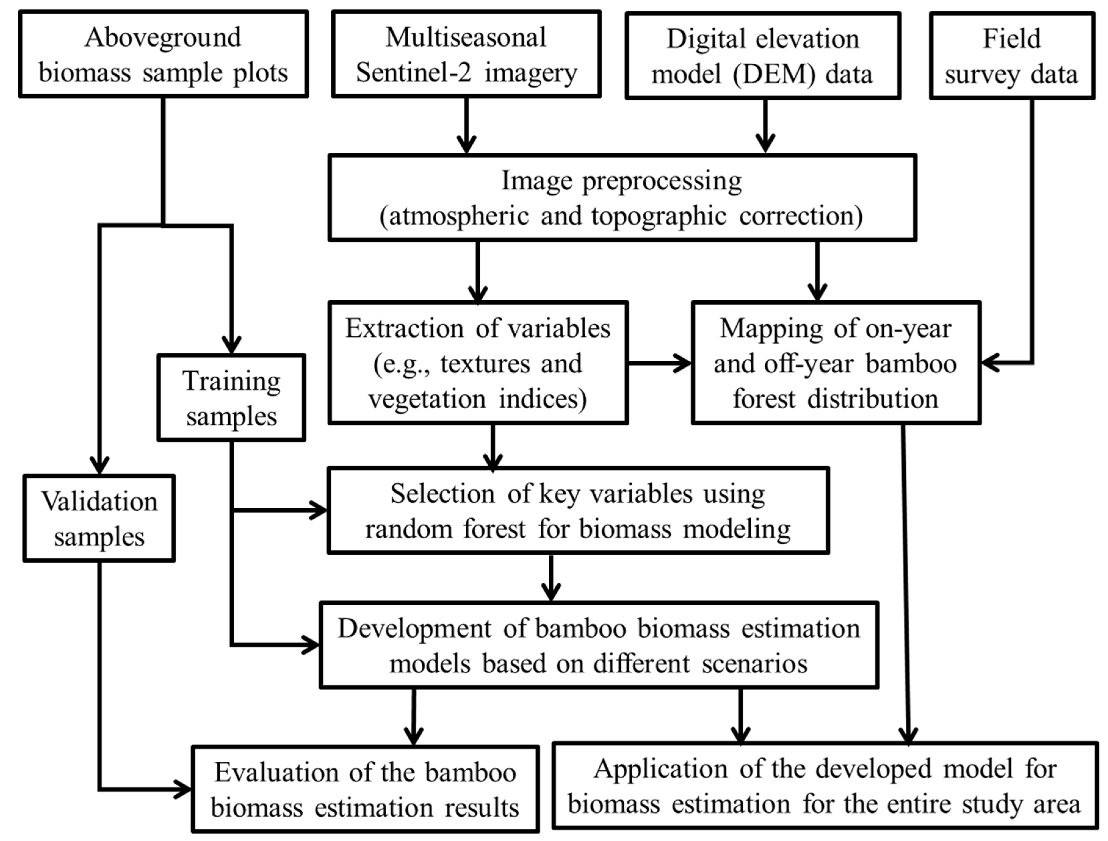
The framework for modeling AGB using Sentinel-2 data is illustrated in Figure 4, including three major steps: (1) Mapping on-year and off-year bamboo forest distribution using multitemporal Sentinel-2 data; (2) extraction of variables from multi-seasonal Sentinel-2 images and selection of key variables using the RF approach; and (3) development of AGB estimation model and evaluation of the modeling results.

2.3. Analysis of Spectral Signature and Mapping of Bamboo Forest Distribution

Accurately mapping bamboo forest distribution is required for bamboo AGB estimation. In order to identify suitable variables for quickly extracting bamboo forests, spectral analysis of on-year and off-year bamboo forests and other forest types was examined based on multitemporal Sentinel-2 images. Compared to Landsat multispectral bands, the Sentinel-2 multispectral bands provide two red edge bands and one NIR band with improved spatial resolution. It is necessary to examine how the newly added spectral bands can separate land-cover types, especially on-year and off-year bamboo forests, which previous research has not examined, probably due to unavailable data sources in the spring season.

As shown in Figure 2, the images acquired in the spring season have obviously different colors for on-year and off-year bamboo forests. Based on the analysis of spectral curves among different dates, a new index based on seasonal images was proposed and a decision tree classifier was then used to map the distribution of on-year and off-year bamboo forests. The Normalized Difference Vegetation Index (NDVI) for winter was first used to mask non-vegetation (e.g., impervious surface, bare soil, croplands, and water) and deciduous forest in the Sentinel-2 image; that is, when NDVI(winter) was less than 0.5, those pixels were masked and the remaining pixels indicated evergreen forests, such as evergreen broadleaf and needle-leaf forests and bamboo forests. The proposed seasonal index was then applied to discriminate on-year and off-year bamboo forests from other evergreen forest types (e.g., teagarden, evergreen broadleaf forest, coniferous forest). The index value of bamboo forests and other forest types is greater than 1 because their spectral values began to increase during the growth season, but the index value of teagarden is less than 1 because teagarden is pruned in May and its spectral value decreases between April and May. In addition, because the spectral value of off-year bamboo forest changes more obviously than other forest types between April and May while the spectral values of on-year bamboo forests are almost unchanged, thresholds can be used to discriminate on-year bamboo, off-year bamboo, and other forest types based on training samples.

Validation sample plots were collected during fieldwork and used to evaluate the classification image. A total of 600 sample plots, including 150 on-year and 150 off-year bamboo forest samples, and 300 other land-cover samples were collected from the field survey data and Google Earth images. The traditional error matrix approach was used to evaluate the classification image [37,38]. Overall accuracy and kappa coefficient were used to evaluate the overall classification performance, and user’s and producer’s accuracies were used to evaluate on-year and off-year bamboo forest classification accuracy.

2.4. Selection of Variables for Development of Biomass Estimation Models

Selection of suitable variables is one of the critical steps in AGB modeling. The most common variables from optical sensor data are spectral responses and textures [12]. Previous research has indicated that the relationships between AGB and spectral responses (spectral bands, vegetation indices) varied, depending on the complexity of forest stand structure and composition of tree species [30]. Spectral bands are fundamental variables for AGB modeling, and proper use of vegetation indices can improve their relationships with AGB [12,30] because external factors such as soil moisture and atmospheric conditions have various impacts on spectral signatures while vegetation indices can reduce these kinds of impacts [39]. Considering the extra red edge spectral bands in the Sentinel-2 data, this research included some vegetation indices that used the red edge wavelength of 750 nm (see

Table 4. A summary of vegetation indices used in research.

Variables	Equations	References
Normalized Different Vegetation index (NDVI)	NDVI = (NIR1 − RED)/(NIR1 + RED)	[41]
Enhance Vegetation index (EVI)	EVI = 2.5(NIR1 − R)/(NIR1 + 6R − 7.5B + 1)	[42]
Soil Adjusted Vegetation Index (SAVI)	SAVI = (NIR1 − R)(1 + L)/(NIR1 + R + L), L = 0.5	[43]
Green Chlorophyll Index (CIgreen)	CIgreen = (NIR1/G) − 1	[44]
Canopy Vegetation Index (CVI)	CVI = (NIR1 − SWIR1)/(NIR1 + SWIR1)	[45]
Simple Ratio (SR)	SR = NIR1/R	[46]
RedEdge Chlorophyll Index (CIre)	CIre = (NIR1/RedEdge1) − 1	[44]
RedEdge Simple Ratio (SRre)	SRre = NIR1/RedEdge1	[47]
RedEdge Normalized Different Vegetation index (NDVIre)	NDVIre = (NIR1 − RedEdge1)/(NIR + RedEdge1)	[47]
MERIS Terrestrial Chlorophyll Index (MTCI)	MTCI = (NIR1 − RedEdge1)/(RedEdge1 − R)	[48]

Note: NIR, near infrared; SWIR, shortwave infrared

for the vegetation indices used in this research), because previous research indicated that this wavelength is more sensitive to vegetation health and chlorophyll contents than other red edge wavelengths [40]. The Pearson’s correlation analysis was used to examine relationships between AGB and these variables.

Spatial feature is another important factor used in AGB modeling. Textural images are often used through a combination of spectral responses [10,11,17]. For effective extraction of a texture image, the spectral band, texture measure, and moving window size must be determined [49]. The GLCM (gray-level co-occurrence matrix) is often used to calculate textural images [10]. Based on our previous research [10,11,17], the textural images were extracted from the first component based on a principal component analysis (PCA) of the Sentinel-2 multispectral images and GLCM measures with a window size of 9 × 9 pixels.

After extraction of variables using vegetation indices and texture measures, another important step is to determine which variables should be used for AGB modeling [13]. Previous research usually used stepwise regression to automatically select variables based on the assumption that the selected variables have no or weak correlation to each other and have a linear relationship with the dependent variable, AGB here. In reality, the remote sensing variables may not have linear relationships with AGB. Thus, we used RF to identify key variables because it can provide the importance ranking of the variables [26]. Some previous studies explored the use of RF for AGB estimation [13] and provided a detailed description of this approach. Therefore, the theory of RF is not described here.

According to the importance ranking of selected variables, Pearson’s correlation analysis was used to examine the relationships between these variables. The backward feature elimination method was used to remove the less important variables while keeping the minimum of root mean squared error (RMSE). By repetitively implementing the RF procedure, we can identify the minimum number of variables but produce the most accurate AGB estimation. A detailed description of the RF-based variable selection and modeling is provided in Gao et al. [13].

After optimization of the parameters in RF, this RF-based model with the finally selected variables was used to estimate bamboo forest AGB for the entire study area. The RF optimization procedure was conducted based on the following scenarios separately: Individual Sentinel-2 data in April, May, and July and combination of all images based on non-stratification (all bamboo forests as one population) and stratification (on-year and off-year groups) for AGB modeling. For non-stratification, 40 samples were used for AGB modeling and 22 samples for validation. For stratification, 20 samples were used for on-year bamboo AGB modeling and 11 samples for AGB estimation validation; the same numbers of samples were used for off-year AGB study. The common evaluation approach with RMSE, relative RMSE (RMSEr), and MAE (mean absolute error) was used, in addition to R². System error (SE) was calculated to examine whether the results were under- or over-estimated. In order to compare the AGB estimation results using different scenarios, Akaike’s Information Criterion (AIC) and Bayesian Information Criterion (BIC) [50,51] were calculated, in which the lowest AIC or BIC value represents the best modeling result.

$$R^2=\frac{{\displaystyle \sum _{i=1}^n{\left(y{e}_i-\overline{ym}\right)}^2}}{{\displaystyle \sum _{i=1}^n{\left(y{m}_i-ym\right)}^2}}$$

(2)

$$RMSE=\sqrt{\frac{{\displaystyle \sum _{i=1}^n{\left(y{e}_i-y{m}_i\right)}^2}}{n}}$$

(3)

$$RMSEr=\frac{RMSE}{\overline{ym}}$$

(4)

$$MAE=\frac{1}{n}{\displaystyle \sum _{i=1}^n\left|y{e}_i-y{m}_i\right|}$$

(5)

$$SE=\frac{1}{n}{\displaystyle \sum _{i=1}^n\left(y{e}_i-y{m}_i\right)}$$

(6)

$$AIC=n\ast \log \left(\frac{SSE}{n}\right)+2K$$

(7)

$$BIC=n\ast \log \left(\frac{SSE}{n}\right)+\log \left(n\right)\ast K$$

(8)

where $y{e}_i$ is the estimated AGB value from the model, $y{m}_i$ is the measured AGB value, $n$ is the number of sampling plots, $\overline{ym}$ is the mean value of the measured AGB value, $SSE$ is the sum of square errors, $K$ is the number of parameters, and $K=p+1$ where $p$ is the number of predictors. Meanwhile, the scatterplots between AGB reference data and estimates and the residual images were used to examine the AGB modeling performance.

3. Results

3.1. Spectral Analysis of On-Year and Off-Year Bamboo Forests and Mapping of Bamboo Distribution

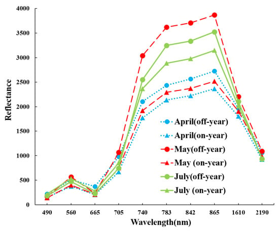
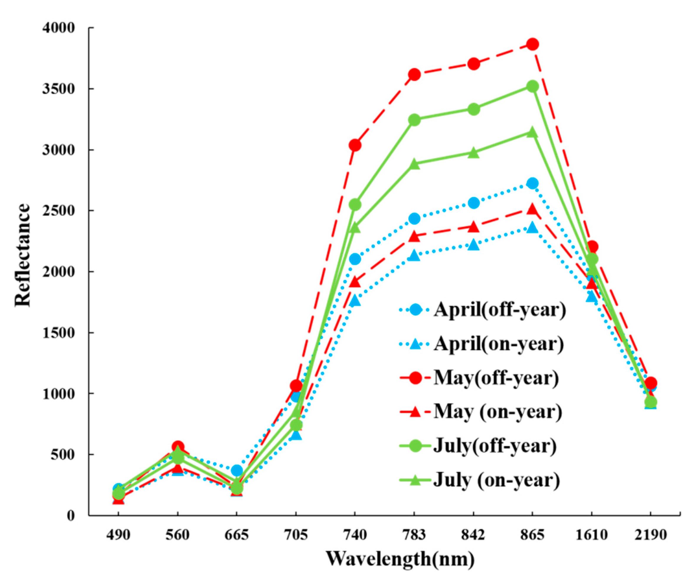
Different spectral signatures of on-year and off-year bamboo forests over time provide the possibility to effectively separate them (Figure 5). In particular, the spectral signatures of on-year and off-year bamboo forests in RedEdge2, RedEdge3, NIR1, and NIR2 (between 740 and 865 nm) have considerably different values in May, indicating that on-year and off-year bamboo forests can be separated, and vegetation indices based on RedEdge2, RedEdge3, NIR1, and NIR2 with visible bands may further improve the separability.

The different spectral curves among the dates indicate the value of using the combination of different dates in classification of on-year and off-year bamboo forests, which previous research had not examined. Based on this idea, a seasonal bamboo index is proposed here:

SBI = (NIR1_S5 + NIR2_S5 + RedEdge3_S5)/(NIR1_S4 + NIR2_S4 + RedEdge3_S4),

(9)

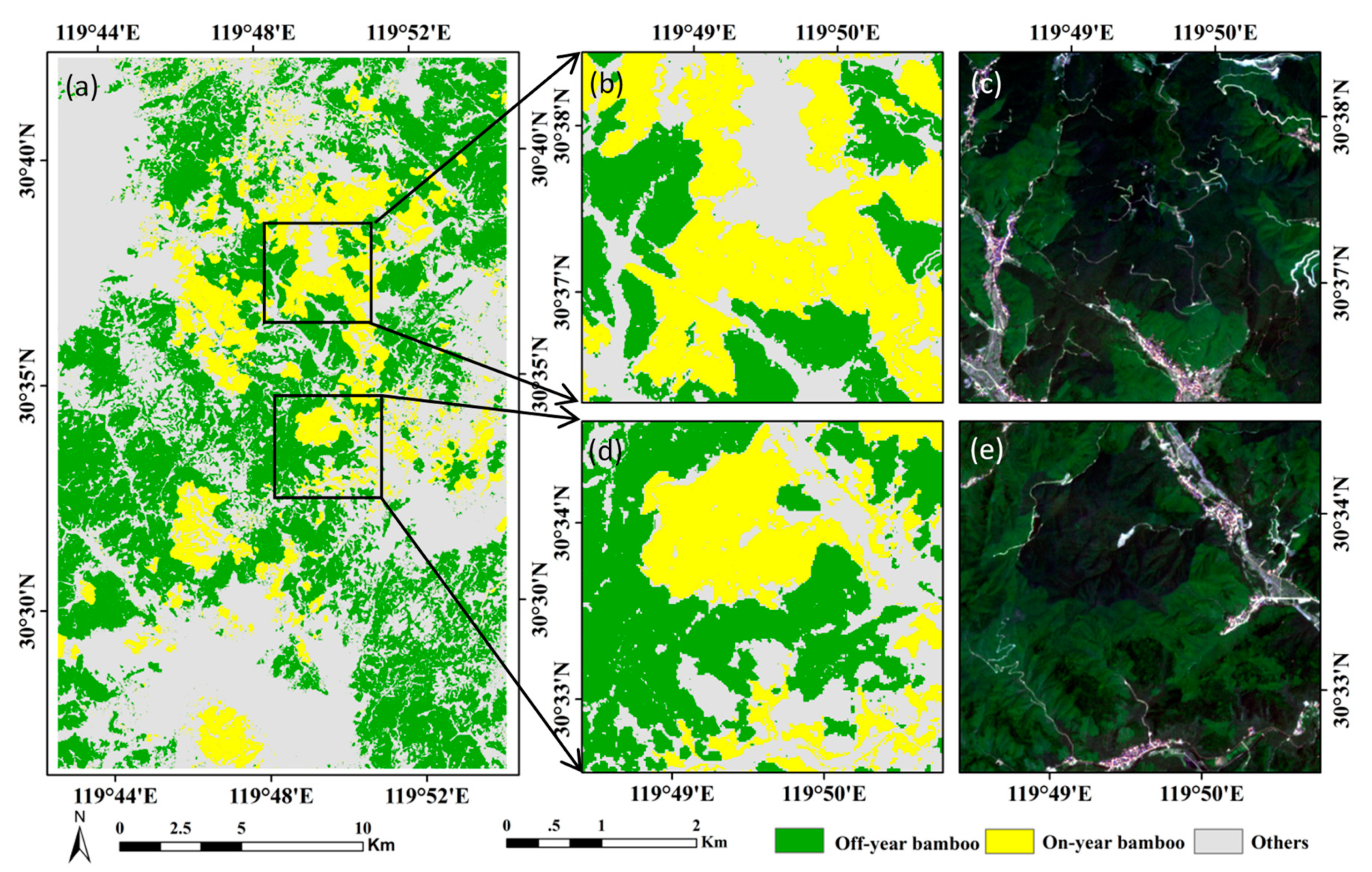
where S5 and S4 represent Sentinel-2 data in May and April. The on-year and off-year bamboo forests in April and May have obvious forest stand structure change, resulting in high variation of SBI compared to other forest types. Therefore, the thresholds of SBI were used to separate on-year and off-year bamboo forests; that is, when SBI > 1.35, the pixels were grouped as off-year bamboo forest, and when SBI < 1.1, the pixels were grouped as on-year bamboo forest. The final results were classified as three classes: On-year bamboo, off-year bamboo, and others, as illustrated in Figure 6. In 2018, the on-year bamboo forests were mainly distributed in the central part of this study area, while off-year bamboo forests were in the southeast, west, and north. The accuracy assessment result (

Table 5. Accuracy assessment results of on-year and off-year bamboo forests classification.

		Reference Data			Producer’s Accuracy	User’s Accuracy	Overall Accuracy
		On-Year Bamboo	Off-Year Bamboo	Others
Classified data	On-year bamboo	140	3	7	93.3	93.3	OCA: 92.6 OKC: 0.88
	Off-year bamboo	1	137	12	90.1	91.3
	Others	9	12	279	92.9	93.0

) indicates that on-year and off-year bamboo forests can be accurately extracted from the bi-seasonal images with producer’s accuracy of 90% to 93% and user’s accuracy of 91% to 93%.

3.2. Correlation Analysis and Identification of Biomass Saturation in Sentinel-2 Data

The correlation coefficients indicate that AGB has different relationships with spectral bands, depending on dates (

Table 6. Pearson’s correlation analysis results.

Bands	Total Samples (62)			On-Year Samples (31)			Off-Year Samples (31)
	April	May	July	April	May	July	April	May	July
Blue	−0.502 **	−0.155	0.229	0.131	0.163	0.04	−0.353	−0.065	0.131
Green	−0.474 **	−0.389 **	0.456 **	0.213	0.166	0.24	0.252	−0.091	0.299
Red	−0.594 **	−0.273 *	0.242	−0.05	0.105	−0.027	−0.502 **	−0.215	0.097
RedEdge1	−0.523 **	−0.424 **	0.488 **	0.083	0.092	0.194	−0.237	0.187	0.376 *
RedEdge2	−0.216	−0.412 **	0.064	0.165	0.149	0.202	0.222	0.253	0.483 **
RedEdge3	−0.028	−0.398 **	−0.053	0.181	0.127	0.157	0.324	0.278	0.442 *
NIR1	−0.096	−0.413 **	−0.01	0.176	0.103	0.171	0.239	0.238	0.423 *
NIR2	−0.105	−0.401 **	−0.038	0.168	0.121	0.156	0.271	0.263	0.438 *
SWIR1	−0.346 **	−0.295 *	0.152	0.083	0.115	0.111	−0.243	0.156	0.448 *
SWIR2	−0.538 **	−0.304 *	0.13	0.095	0.136	0.069	−0.503 **	−0.04	0.219

** significance at 0.01 both-side confidential level; * significance at 0.05 both-side confidential level.

). For example, in April, visible, RedEdge1, and SWIR bands have significant correlations with AGB, but RedEdge2, RedEdge3, NIR1, and NIR2 bands do not. In May, all spectral bands except blue have significant correlations with AGB; in particular, the red edge and NIR bands have stronger correlation with AGB than visible and SWIR bands; however, in July, only green and RedEdge1 have a significant correlation with AGB. One interesting thing is in the on-year bamboo forests, no spectral bands have a significant correlation with AGB, whether in April, May or July, while in off-year bamboo forests, only red and SWIR2 bands have a significant correlation with AGB in April, but none do in May. On the other hand, in July, the spectral bands from RedEdge1 to SWIR1 (705–1610 nm) have a significant correlation with AGB. The correlation coefficients in Table 6 show that the on-year bamboo forests do not have linear relationships with AGB, implying that traditional linear regression models are not suitable for on-year bamboo AGB estimation; however, with proper selection of seasonal image and spectral bands, linear regression may be suitable for off-year bamboo AGB estimation. In contrast, if both on-year and off-year bamboo forests are combined as one population, the high correlation coefficients (0.52–0.59) between AGB and red, RedEdge1, and SWIR in the April image may imply that the April image provides the most accurate AGB estimation.

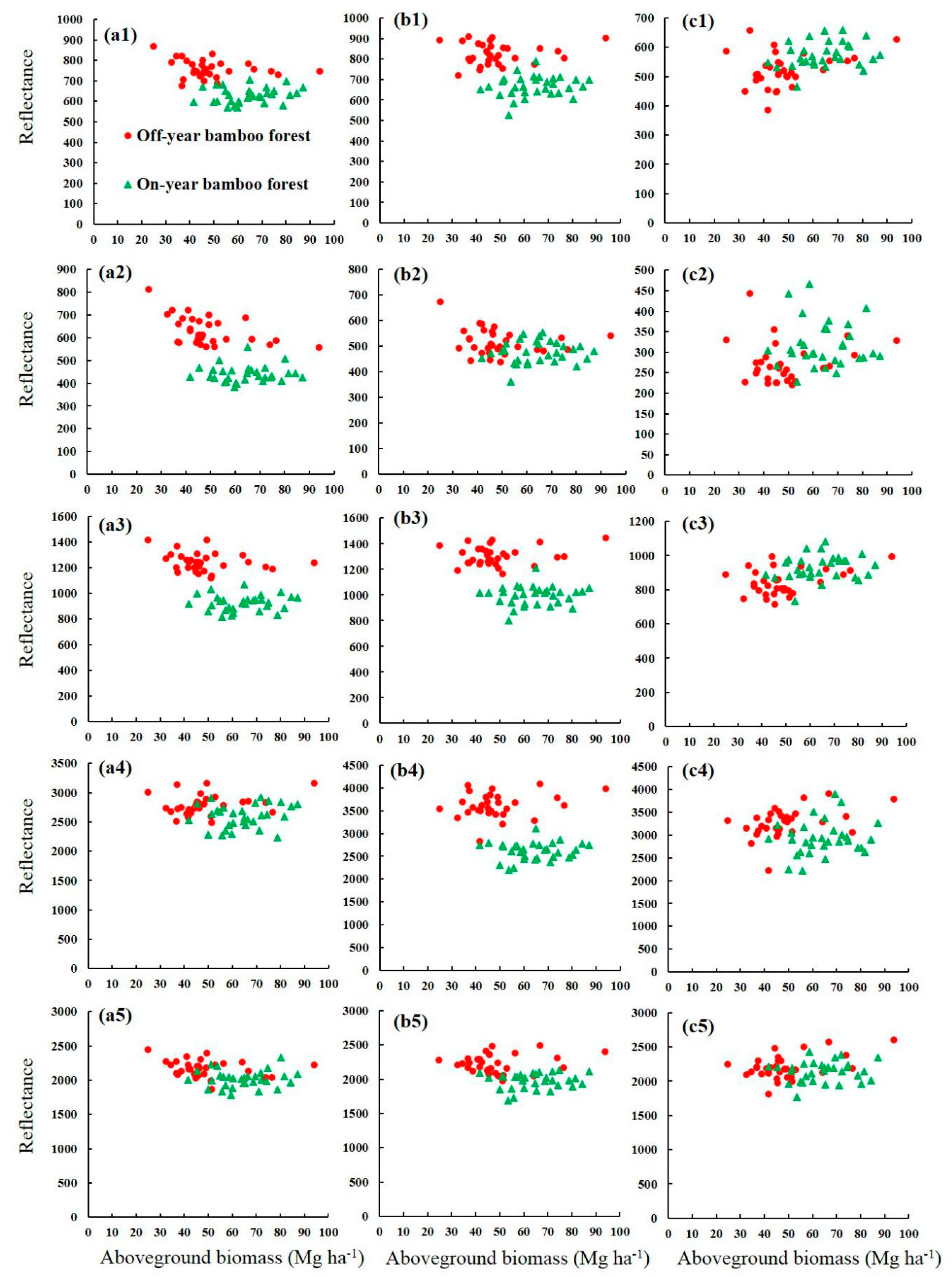
The relationships between spectral bands and AGB are illustrated in scatterplots (Figure 7). For on-year bamboo forests, the correlation results in Table 6 show that spectral bands have no relationships with AGB, and Figure 7 confirms that even as AGB increases from about 40 to about 90 Mgha⁻¹, their spectral values remain almost the same, implying that spectral bands cannot be used for on-year bamboo AGB estimation. For off-year bamboo forests, as AGB increases, spectral values in green, red, and RedEdge1 decease to AGB values of about 50 Mgha⁻¹ in April and May. In contrast, as AGB increases, spectral values of green and red bands in July increase, while spectral values in NIR and SWIR bands are almost the same in April, May, and July, even as AGB increases. This implies that visible bands may be used for off-year bamboo AGB estimation, but because of data saturation (when AGB is greater than about 50 Mgha⁻¹) spectral values cannot be effectively used for AGB estimation.

Figure 7 also indicates that with the combination of on-year and off-year bamboo forest as one population, the linear relationships between AGB and spectral bands in green, red, and RedEdge1 in April, green, RedEdge1, and NIR1 in May, and green and RedEdge1 in July have obviously linear relationships until AGB reaches about 60 Mgha⁻¹. The better linear relationships and higher AGB saturation values in the combination of on-year and off-year bamboo forest than in on-year or off-year alone imply that stratification of on-year and off-year bamboo forests may not be necessary.

3.3. Identification of Key Variables for Biomass Modeling

The key variables identified using RF (

Table 7. A summary of key variables used in random forest.

Dates	Variables	Non-Stratification			Variables	On-Year Bamboo			Variables	Off-Year Bamboo
		R2	MAE	RMSE		R2	MAE	RMSE		R2	MAE	RMSE
Comb. seasons	EVIS4, SRS4, RedEdge1S7	0.86	5.37	6.59	BlueS5, SWIR2S7, SWIR2S5	0.84	4.51	5.60	SWIR2S4, EVIS4, SWIR1S7	0.85	5.32	7.04
April	EVIS4, TW9SECS4, SWIR2S4, TW9VAS4	0.90	4.90	5.94	SRS4, NDVIreS4, REDS4	0.75	5.73	7.20	RedS4, SWIR2S4, SRreS4, EVIS4	0.85	5.73	7.25
May	RedS5, BlueS5, TW9MES5	0.86	5.62	7.13	BlueS5, RedS5, SWIR2S5, EVIS5	0.89	4.40	5.30	SWIR1S5, CIgreenS5, TW9MES5	0.78	6.69	8.77
July	RedEdge1S7, CIgreenS7, MTCIS7	0.89	5.41	7.03	SWIR2S7, SRreS7, CVIS7	0.84	5.61	6.75	NIR2S7, SWIR1S7, TW9ENS7	0.84	6.08	7.67

Note: NIR, near infrared; SWIR, shortwave infrared; RedEdge, vegetation red edge band; S4, Sentinel-2 multispectral data in April; S5, Sentinel-2 multispectral data in May; S7, Sentinel-2 multispectral data in July; NDVI, normalized difference vegetation index; T, texture. Different texture measures: EN, entropy; SEC, second moment; ME, mean; VA, variance; EVI, enhanced vegetation index; CIgreen, green chlorophyll index; CVI, canopy vegetation index; MTCI, MERIS terrestrial chlorophyll index; SR_RE, RedEdge simple ratio; SR, simple ratio.

) indicate that spectral responses (spectral bands and vegetation indices) are more important than textures in bamboo AGB modeling according to the importance ranking. Under the non-stratification condition, one texture in May and two textures in April were selected, but no textures were selected in July or in the combination of multiple seasons. With stratification of on-year and off-year bamboo forests, no textures were selected for on-year bamboo AGB modeling, and only one texture was selected in off-year bamboo AGB modeling using the May or July imagery. Table 7 implies that texture may not be a critical variable in bamboo AGB modeling. Although Figure 7 indicates that AGB has weak linear correlation with most of the spectral bands, especially for the on-year bamboo forests, the high R² and relatively low MAE and RMSE values in Table 7 imply that the RF-based approach may be valuable for bamboo AGB estimation. For example, in non-stratification, the April image provides the best overall AGB estimation performance, the May image provides the best performance for on-year bamboo forest, and the combination of April and July imagery provides the most accurate estimation for off-year bamboo forest.

3.4. Analysis of Bamboo Forest Biomass Estimation Results

The accuracy assessment results (

Table 8. Evaluation of estimation results using the non-stratification- and stratification-based models.

Data	Evaluation of Estimation Using Non-Stratified Models						Evaluation of Estimation Using Stratified Models
	R2	RMSE	RMSEr	MAE	AIC	BIC	R2	RMSE	RMSEr	MAE	AIC	BIC
Comb. seasons	0.24	12.97	23.17%	9.91	54.96	52.99	0.34	12.00	21.45%	9.35	53.49	51.52
April	0.43	11.44	20.45%	9.43	54.28	51.95	0.25	12.72	22.72%	10.84	55.59	53.29
May	0.15	13.44	24.02%	10.81	55.65	53.68	0.29	12.35	22.07%	9.93	55.03	52.73
July	0.13	14.12	25.23%	10.77	56.59	54.62	0.46	10.68	19.09%	8.56	51.26	49.29

Note: R²—coefficient of determination; RMSE, RMSEr, and MAE—root mean squared error, relative root mean squared error, and mean absolute error; AIC and BIC—Akaike’s Information Criterion and Bayesian Information Criterion.

) show that under the non-stratification condition, the April image provides the best estimation performance with the highest R² value and lowest values of other evaluation parameters (e.g., RMSE, RMSEr, MAE, AIC and BIC). The overall estimation results based on this stratification condition using the July image slightly improved the AGB estimation over the best estimation with non-stratification using the April image. On the other hand, the highest R² value (0.46) and the lowest error evaluation parameter values imply that the stratification-based AGB estimation model using the July image can predict the best AGB estimates

When this non-stratification-based AGB model was used to map the entire study area, the April image also provided the lowest errors for both on-year or off-year bamboo AGB estimations. The combination of April and July images did not improve AGB estimation performance compared to the April image alone. Although the RMSE, RMSEr, and MAE for on-year and off-year bamboo forests in April have small values using the non-stratification-based AGB model, the low R² values (0.05 for on-year and 0.03 for off-year) may imply poor estimation results because the estimates and reference data do not have a good linear relationship. With stratification of on-year and off-year bamboo forests, the AGB modeling using the July image based on either on-year or off-year bamboo samples, the RMSE and RMSEr are the lowest values compared to the April and May images, and combination of multiple dates of images cannot improve AGB estimation performance. The off-year bamboo AGB estimation based on the stratification indeed considerably improved estimation performance, with RMSE of 7.75 Mgha⁻¹ and RMSEr of 17.88% using the July image, compared to non-stratification with RMSE of 10.0–14.6 Mgha⁻¹ and RMSEr of 23.1% to 33.7%. For on-year bamboo AGB estimation, the estimation results between stratification and non-stratification did not differ much; for example, RMSE was 13–14.1 Mgha⁻¹ and RMSEr was 18.9% to 20.6% for stratification, and 12.7–15.1 Mgha⁻¹, 18.5% to 22.1% for non-stratification, implying the difficulty of AGB estimation for on-year bamboo forest using the Sentinel-2 data.

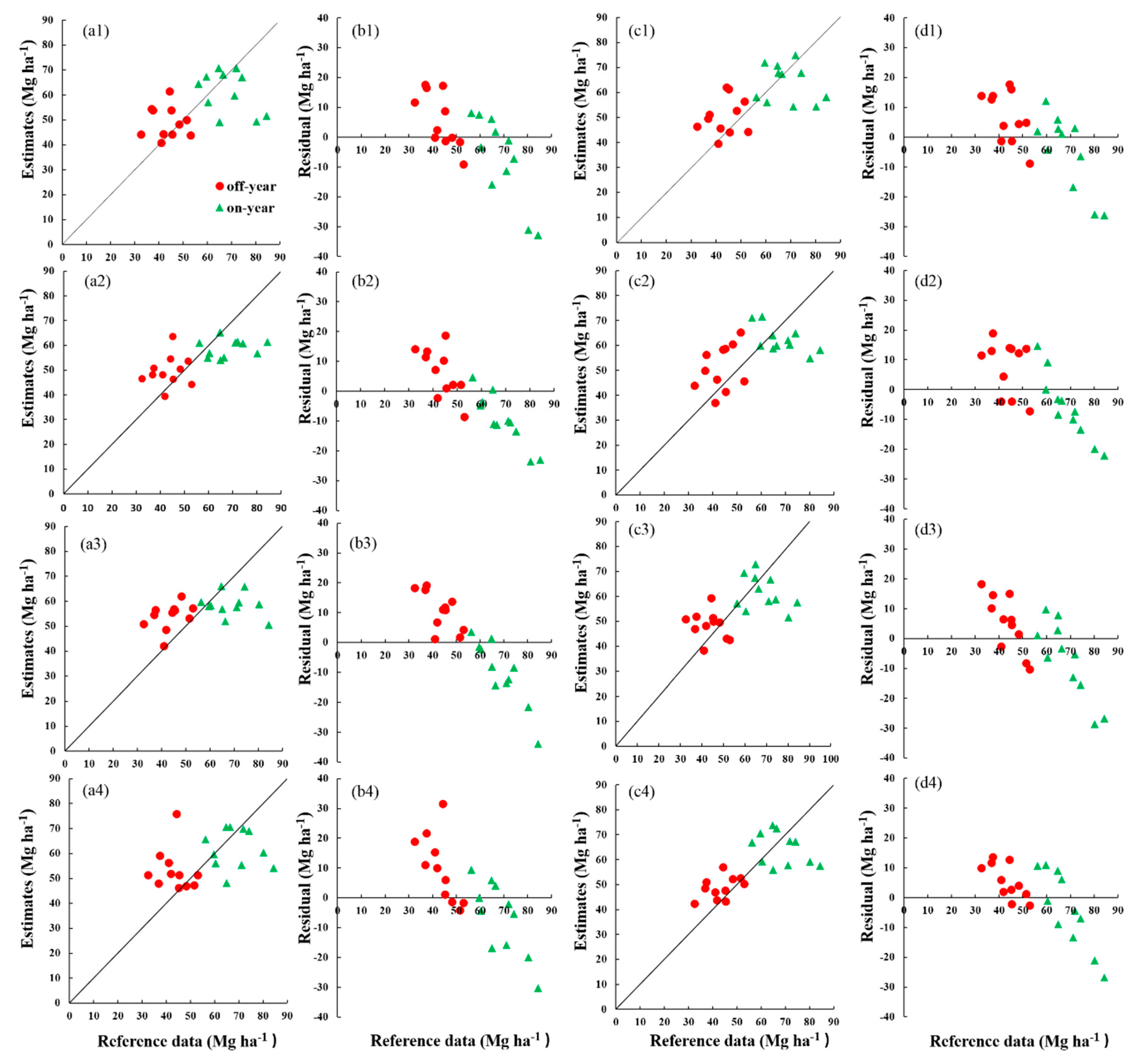
The scatterplots in Figure 8 indicate that the off-year bamboo forests are more prone to be overestimated, especially when AGB is less than 40 Mgha⁻¹, while on-year bamboo forests are more apt to be underestimated. This situation is especially serious when AGB is greater than 70 Mgha⁻¹ because of the data saturation problem as illustrated in Figure 7. Comparing the residual results between non-stratification and stratification models, the under- or over-estimation problems were slightly reduced but still very obvious in the stratification-based models. For example, when AGB is greater than 80 Mgha⁻¹, the underestimation value can be over 30 Mgha⁻¹ (Figure 8).

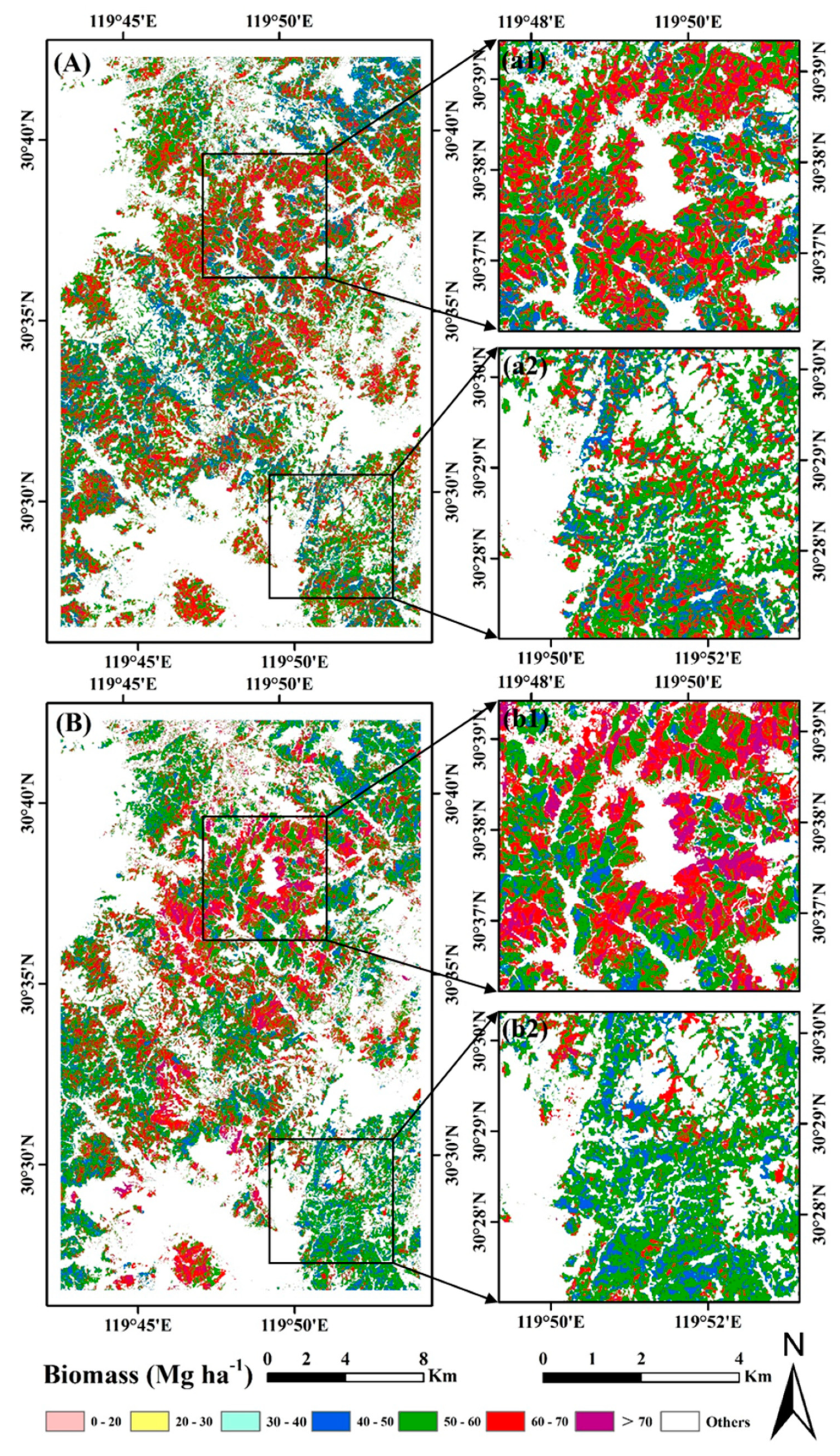
The spatial distributions of the predicted AGB using the most accurate AGB models under non-stratification and stratification conditions are illustrated in Figure 9. Comparison of Figure 9 and Figure 6 indicates that the lower right region in Figure 9a2 has many more AGB pixels with high AGB values than the same region in Figure 9b2, confirming more accurate estimation using the stratification-based AGB model for off-year bamboo forest AGB estimation, which is confirmed in

Table 9. Evaluation of estimation results based on non-stratification- and stratification-based models using the on-year and off-year validation samples.

	Evaluation of Estimation Results Based on Non-Stratification Models
Data	Evaluation Using On-Year Samples				Evaluation Using Off-Year Samples
	R2	RMSE	RMSEr	MAE	R2	RMSE	RMSEr	MAE
Comb	0.24	15.12	22.05%	11.52	0.01	10.37	23.92%	8.31
April	0.05	12.71	18.53%	10.54	0.03	10.02	23.11%	8.31
May	0.06	14.51	21.16%	11.00	0.16	12.27	28.33%	10.63
July	0.01	13.62	19.86%	11.17	0.02	14.60	33.69%	10.37
Evaluation of Estimation Results Based on Stratified Models
Data	Evaluation Using On-Year Samples				Evaluation Using Off-Year Samples
	R2	RMSE	RMSEr	MAE	R2	RMSE	RMSEr	MAE
Comb	0.05	13.17	19.20%	9.68	0.04	10.71	24.71%	9.00
April	0.42	13.71	20.00%	11.06	0.13	11.64	26.85%	10.63
May	0.12	14.12	20.59%	10.93	0.06	10.28	23.72%	8.92
July	0.16	12.97	18.91%	10.89	0.20	7.75	17.88%	6.24

. Based on analysis of system errors, on-year bamboo AGB is underestimated, and off-year bamboo AGB is overestimated (

Table 10. Comparison of system errors for on-year and off-year bamboo forest biomass estimation based on non-stratification and stratification conditions.

	On-Year	Off-Year
Non-stratification model in April	−9.61	+6.32
Stratification model in July	−4.20	+5.37

). The stratification-based AGB modeling approach is especially valuable in reducing the on-year underestimation problem.

4. Discussion

4.1. Impacts of Phenological Features of Bamboo Forests on Biomass Estimation Performance

In general, broadleaf and coniferous forests have relatively stable stand structures month to month or even year to year if no serious disturbance is inflicted by external factors, such as selective logging or serious drought. Therefore, previous studies often collected AGB field measurements and remotely sensed data for AGB modeling on different dates due to the difficulty of acquiring data sources during the same year [10,11,17]. However, bamboo forests change their canopies and structures rapidly, especially in spring due to the rapid growth from shoots to fully developed trees, and during fall and winter seasons due to selective logging of old trees (3 du or older). Therefore, the spectral values at different image acquisition dates have high variation due to the bamboo phenological characteristics, as shown in Figure 2 and Figure 5. Thus, the inconsistency of dates between field measurements and image acquisition for AGB calculation may considerably affect the relationships between the spectral bands and AGB, and even produce spurious relationships [13]. Another big difference between bamboo and other forest types is that bamboo forests have on-year and off-year growth features (see Figure 1), while other forest types do not. As shown in this research, the on-year bamboo forests can seriously affect AGB modeling effects due to the low AGB data saturation problem; that is, on-year bamboo forests may have high AGB variation, but their spectral signatures are very similar, and there are no significant relationships between on-year bamboo AGB and spectral responses, as shown in Table 6. This implies that the spectral bands are not suitable for on-year bamboo AGB modeling, especially the traditional linear regression models. More research is needed to use high spatial resolution images (e.g., QuickBird, WorldView) with better than 2 m to examine how changes in stand structure of on-year bamboo forests influence the relationships between AGB and spectral signatures.

4.2. The Potential to Improve Biomass Estimation Performance

Many previous studies have indicated that the combination of spectral responses and textures is valuable to improve AGB estimation performance, either in tropical or subtropical forest types [11,13,14,15]. However, our research indicates that textures are not critical variables for AGB estimation in bamboo forests. This may be due to the fact that bamboo forests have a single tree species with similar DBH, height, and stand structure. Thus, in bamboo AGB, the tree age and density caused by on-year and off-year phenology play important roles.

The challenge in bamboo AGB estimation is the difficulty in modeling on-year bamboo AGB because of the serious data saturation problem. Previous studies [1,2,10,11,14,20] as well as this study confirm the difficulty of using optical sensor data, and the RMSEr can be over 20%. Incorporation of remotely sensed data and ancillary data such as soil and topographic factors may improve AGB estimation if proper modeling algorithms, such as support vector machine, are used [17]. The common approaches, such as machine learning algorithms, that are valid for broadleaf and coniferous AGB modeling may not be suitable for bamboo AGB modeling due to their completely different growth characteristics. Researchers need to develop new algorithms that can effectively incorporate the bamboo forest’s growth stage information, such as how shoots grow quickly to fully developed trees causing a rapid increase in AGB within two to three months.

Optical sensor data can only provide land surface information and cannot provide vertical forest stand structure information. Previous research using optical or radar data for AGB modeling has indicated that data saturation is an important factor resulting in poor estimation performance [10,11,17]. This research also indicates that when bamboo forest AGB is greater than 70 Mgha⁻¹, Sentinel-2 data cannot effectively estimate off-year bamboo forest and yield very high underestimation values, especially for on-year bamboo forests. Previous research has shown that incorporating tree height can solve the data saturation problem; thus, using lidar or satellite stereo images can considerably improve AGB estimation [52]. However, bamboo forests have very different growth characteristics from other forest types, as described in the Introduction. The AGB in different bamboo forest sites may be considerably different, but their average DBH and canopy height can be similar. The difference in AGB is mainly caused by different bamboo ages and tree densities. Therefore, use of lidar or stereo images for bamboo AGB estimation may not be as helpful as for other forest types. Researchers need to develop new approaches to extract from bamboo forests the ages and densities of the trees. Bamboo age is related to tree density, because the increase in tree density is due to new bamboo shoots in the on-year bamboo forests. The Sentinel-2 or Landsat images with spatial resolution of 10 or lower cannot effectively capture the subtle difference in tree densities. Higher spatial resolution images such as QuickBird, WorldView, and Pleiades with sub-meter spatial resolution may be needed. To date, there are no such studies for bamboo AGB modeling. In the near future, we need to explore how the very high spatial resolution images can be used for bamboo forest AGB estimation. The available high-speed computers and sub-meter resolution satellite images provide a new opportunity for improvements. In particular, use of the Unmanned Aerial Vehicle (UAV) may provide a new way to estimate bamboo AGB.

5. Conclusions

Remote sensing-based bamboo AGB estimation has been extensively explored, but the estimation accuracy often has been very poor due to poor understanding of the impacts of the bamboo forest growth characteristics on remote sensing spectral signatures. This research examined using multiple dates of Sentinel-2 multispectral images in bamboo forest classification and AGB estimation based on stratification of on-year and off-year bamboo forests. This research identified the major problems that affect bamboo AGB estimation performance: Mismatch of dates of AGB sample collection and acquisition of remotely sensed data, the high variation of the bamboo stand structures within one year caused by rapid growth from shoots to full-size trees and selective logging, the on-year and off-year bamboo growth features, and the AGB saturation in optical sensor data, especially for the on-year bamboo forest. The on-year bamboo forests have a serious data saturation problem, thus, optical sensor data such as Landsat and Sentinel-2 are not suitable for on-year bamboo AGB estimation. The off-year bamboo forests had obviously linear relationships with AGB, especially when the July Sentinel-2 data were used; the estimation RMSE can be as low as 7.75 Mgha⁻¹. If an insufficient number of samples is available for on-year and off-year bamboo forests, the non-stratification-based AGB model using the April image can provide the most accurate estimation results. This research indicates the difficulty in using optical sensor data alone for bamboo forest AGB estimation. More research should be explored to incorporate multiple data sources such as lidar, optical sensor multispectral data, and ancillary data into AGB modeling. An alternative is to use very high spatial resolution images such as Pleiades and WorldView with sub-meter resolution for extraction of tree density that can be incorporated into the AGB estimation models.

References

- Zhou, G.; Meng, C.; Jiang, P.; Xu, Q. Review of carbon fixation in bamboo forests in China. Bot. Rev. 2011, 77, 262–270. [Google Scholar] [CrossRef]
- Du, H.; Zhou, G.; Ge, H.; Fan, W.; Xu, X.; Fan, W.; Shi, Y. Satellite-based carbon stock estimation for bamboo forest with a non-linear partial least square regression technique. Int. J. Remote Sens. 2012, 33, 1917–1933. [Google Scholar] [CrossRef]
- Yen, T. Culm height development, biomass accumulation and carbon storage in an initial growth stage for a fast-growing Moso bamboo (Phyllostachypubescens). Bot. Stud. 2016, 57, 10–19. [Google Scholar] [CrossRef] [PubMed]
- Chen, X.; Zhang, Y.; Zhang, X.; Kuo, Y. Carbon stock changes in bamboo stands in China over the last 50 years. Acta Ecol. Sin. 2008, 8, 5218–5227. [Google Scholar]
- Zhou, G.; Xu, X.; Du, H.; Ge, H.; Shi, Y.; Zhou, Y. Estimating aboveground carbon of Moso bamboo forests using the k nearest neighbor’s technique and satellite imagery. Photogramm. Eng. Remote Sens. 2011, 77, 1123–1131. [Google Scholar] [CrossRef]
- Song, X.; Zhou, G.; Jiang, H.; Yu, S.; Fu, J.; Li, W.; Wang, W.; Ma, Z.; Peng, C. Carbon sequestration by Chinese bamboo forests and their ecological benefits: Assessment of potential, problems, and future challenges. Environ. Rev. 2011, 19, 418–428. [Google Scholar] [CrossRef]
- Nath, A.; Lal, R.; Das, A. Managing woody bamboos for carbon farming and carbon trading. Glob. Ecol. Conserv. 2015, 3, 654–663. [Google Scholar] [CrossRef]
- Du, H.; Sun, X.; Han, N.; Mao, F. RS estimation of inventory parameters and carbon storage of Moso bamboo forest based on synergistic use of object-based image analysis and decision tree. J. Appl. Ecol. 2017, 8, 3163–3173. [Google Scholar] [CrossRef]
- Fang, W.; Gui, R.; Ma, L.; Jin, A.; Lin, X.; Yu, X.; Qian, J. Chinese Economic Bamboo, 1st ed.; Science Press: Beijing, China, 2015; pp. 104–109. ISBN 9787030454607. [Google Scholar]
- Zhao, P.; Lu, D.; Wang, G.; Wu, C.; Huang, Y.; Yu, S. Examining spectral reflectance saturation in Landsat imagery and corresponding solutions to improve forest aboveground biomass estimation. Remote Sens. 2016, 8, 469. [Google Scholar] [CrossRef]
- Zhao, P.; Lu, D.; Wang, G.; Wu, C.; Huang, Y.; Yu, S. Forest aboveground biomass estimation in Zhejiang Province using the integration of Landsat TM and ALOS PALSAR data. Int. J. Appl. Earth Obs. Geoinf. 2016, 53, 1–15. [Google Scholar] [CrossRef]
- Lu, D.; Chen, Q.; Wang, G.; Liu, L.; Li, G.; Moran, E. A survey of remote sensing–based aboveground biomass estimation methods in forest ecosystems. Int. J. Earth. 2016, 9, 63–105. [Google Scholar] [CrossRef]
- Gao, Y.; Lu, D.; Li, G.; Wang, G.; Chen, Q.; Liu, L.; LI, D. Comparative analysis of modeling algorithms for forest aboveground biomass estimation in a subtropical region. Remote Sens. 2018, 10, 627. [Google Scholar] [CrossRef]
- Xu, X.; Zhou, G.; Du, H.; Zhou, Y.; Hu, J.; Lu, G. Effect of sample plots stratification on estimation accuracy of aboveground carbon storage for Phyllostachysedulis forest. Sci. Silvae Sin. 2013, 49, 18–24. [Google Scholar] [CrossRef]
- Du, H.; Cui, R.; Zhou, G.; Shi, Y.; Xu, X.; Fan, W.; Lü, Y. The responses of Moso bamboo (Phyllostachys Pubescens) forest aboveground biomass to Landsat TM spectral reflectance and NDVI. Acta Ecol. Sin. 2010, 30, 257–263. [Google Scholar] [CrossRef]
- Cui, R.; Du, H.; Zhou, G.; Xu, X.; Dong, D.; Lü, Y. Remote sensing–based dynamic monitoring of Moso bamboo forest and its carbon stock change in Anji County. J. Zhejiang A F Univ. 2011, 28, 422–431. [Google Scholar]
- Lu, D. The potential challenge of remote sensing–based biomass estimation. Int. J. Remote Sens. 2006, 27, 1297–1328. [Google Scholar] [CrossRef]
- Lu, D.; Batistella, M. Exploring TM image texture and its relationships with biomass estimation in Rondônia, Brazilian Amazon. Acta Amazonica 2005, 35, 249–257. [Google Scholar] [CrossRef]
- Lu, D.; Batistella, M.; Moran, E. Satellite estimation of aboveground biomass and impacts of forest stand structure. Photogramm. Eng. Remote Sens. 2005, 71, 967–974. [Google Scholar] [CrossRef]
- Han, N.; Du, H.; Zhou, G.; Xu, X.; Cui, R.; Gu, C. Spatiotemporal heterogeneity of Moso bamboo aboveground carbon storage with Landsat Thematic Mapper images: A case study from Anji County, China. Int. J. Remote Sens. 2013, 34, 4917–4932. [Google Scholar] [CrossRef]
- Yu, Z.; Du, H.; Zhou, G.; Xu, X.; Gui, Z. Transferability of remote sensing–based models for estimating Moso bamboo forest aboveground biomass. J. Appl. Ecol. 2012, 23, 2422–2428. [Google Scholar] [CrossRef]
- Avitabile, V.; Baccini, A.; Friedl, M.A.; Schmullius, C. Capabilities and limitations of Landsat and land cover data for aboveground woody biomass estimation of Uganda. Remote Sens. Environ. 2012, 117, 366–380. [Google Scholar] [CrossRef]
- Baccini, A.; Laporte, N.; Goetz, S.J.; Sun, M.; Dong, H. A first map of tropical Africa’s aboveground biomass derived from satellite imagery. Environ. Res. Lett. 2008, 3, 045011. [Google Scholar] [CrossRef]
- Pflugmatcher, D.; Cohen, W.B.; Kennedy, R.E.; Yang, Z. Using Landsat-derived disturbance and recovery history and lidar to map forest biomass dynamics. Remote Sens. Environ. 2014, 151, 124–137. [Google Scholar] [CrossRef]
- Tanase, M.A.; Panciera, R.; Lowell, K.; Tian, S.; Hacker, J.M.; Walker, J.P. Airborne multi-temporal L-band polarimetric SAR data for biomass estimation in semi-arid forests. Remote Sens. Environ. 2014, 145, 93–104. [Google Scholar] [CrossRef]
- Breiman, L. Random Forests. Mach. Learn. 2001, 45, 5–32. [Google Scholar] [CrossRef] [Green Version]
- Ismail, R.; Mutanga, O.; Kumar, L. Modeling the potential distribution of pine forests susceptible to SirexNoctilio infestations in Mpumalanga, South Africa. Trans. GIS. 2010, 14, 709–726. [Google Scholar] [CrossRef]
- Vincenzi, S.; Zucchetta, M.; Franzoi, P.; Pellizzato, M.; Pranovi, F.; De Leo, G.A.; Torricelli, P. Application of a Random Forest algorithm to predict spatial distribution of the potential yield of Ruditapes Philippinarum in the Venice lagoon, Italy. Ecol. Model. 2011, 222, 1471–1478. [Google Scholar] [CrossRef]
- Lu, D. Aboveground biomass estimation using Landsat TM data in the Brazilian Amazon. Int. J. Remote Sens. 2005, 26, 2509–2525. [Google Scholar] [CrossRef]
- Lu, D.; Mausel, P.; Brondízio, E.; Moran, E. Relationships between forest stand parameters and Landsat Thematic Mapper spectral responses in the Brazilian Amazon Basin. For. Ecol. Manag. 2004, 198, 149–167. [Google Scholar] [CrossRef]
- Zhang, L. The Estimation of Gross Primary Production of Phyllostachys Pubescens Based on MODIS and Eddy Covariance Flux Data in Zhejiang Anji. Master’s Thesis, Zhejiang A&F University, Hangzhou, China, 2013. [Google Scholar]
- Cui, R. Satellite-Based Spatiotemporal Variation of Carbon Storage of Moso Bamboo Forest in Anji County. Master’s Thesis, Zhejiang A&F University, Hangzhou, China, 2011. [Google Scholar]
- Anji Forestry Bureau. Anji County Forestry Resources Survey Results Report; Anji Forestry Bureau: Anji, China, 2016.
- Zhou, G. Carbon Storage, Ixation and Distribution in Moso Bamboo (Phyllostachys pubescens) Stands Ecosystem. Ph.D. Thesis, Zhejiang University, Hangzhou, China, 2006. [Google Scholar]
- Muller-Wilm, U.; Louis, J.; Richter, R.; Gascon, F.; Niezette, M. Sentinel-2 Level 2A Prototype Processor: Architecture, Algorithms and First Results. ESA Spec. Publ. 2013, 722, 2–13. [Google Scholar]
- Sola, I.; González-Audícana, M.; Álvarez-Mozos, J. Multi-criteria evaluation of topographic correction methods. Remote Sens. Environ. 2011, 184, 247–262. [Google Scholar] [CrossRef]
- Foody, G. Status of land cover classification accuracy assessment. Remote Sens. Environ. 2002, 80, 185–201. [Google Scholar] [CrossRef]
- Foody, G. Assessing the Accuracy of Remotely Sensed Data: Principles and Practices. Photogramm. Rec. 2010, 25, 204–205. [Google Scholar] [CrossRef]
- Finley, A.O.; Munoz, J.D.; Gehl, R. Nonlinear hierarchical models for predicting cover crop biomass using Normalized Difference Vegetation Index. Remote Sens. Environ. 2010, 114, 2833–2840. [Google Scholar] [CrossRef]
- Zheng, Y.; Wu, B.; Zhang, M. Estimating the aboveground biomass of winter wheat using the Sentinel-2 data. J. Remote Sens. 2017, 21, 318–328. [Google Scholar] [CrossRef]
- Tucker, C. Red and photographic infrared linear combinations for monitoring vegetation. Remote Sens. Environ. 1979, 8, 127–150. [Google Scholar] [CrossRef] [Green Version]
- Liu, H.; Huete, R. A Feedback based modification of the NDVI to minimize canopy background and atmosphere noise. IEEE Trans. Geosci. Remote Sens. 1995, 33, 457–465. [Google Scholar] [CrossRef]
- Huete, R. A Soil-adjusted vegetation index (SAVI). Remote Sens. Environ. 1988, 25, 295–309. [Google Scholar] [CrossRef]
- Gitelson, A.; Vina, A.; Ciganda, V.; Rundquist, D.; Arkebauer, J. Remote estimation of canopy chlorophyll content in crops. Geophys. Res. Lett. 2005, 32, 93–114. [Google Scholar] [CrossRef]
- Xu, R.; Ma, Y.; He, C. Remote Sensing Biogeochemistry, 2nd ed.; Guangdong Science and Technology Press: Guangzhou, China, 2003; pp. 99–103. ISBN 9787535932143. [Google Scholar]
- Jordan, C. Derivation of leaf-area index from quality of light on the forest floor. Ecology 1969, 50, 663–666. [Google Scholar] [CrossRef]
- Sims, D.; Gamon, J. Relationships between leaf pigment content and spectral reflectance across a wide range of species, leaf structures and developmental stages. Remote Sens. Environ. 2002, 81, 337–354. [Google Scholar] [CrossRef]
- Dash, J.; Curran, P.J. The MERIS terrestrial chlorophyll index. Int. J. Remote Sens. 2004, 25, 5403–5413. [Google Scholar] [CrossRef]
- Lu, D.; Li, G.; Moran, E.; Dutra, L.; Batistella, M. The roles of textural images in improving land-cover classification in the Brazilian Amazon. Int. J. Remote Sens. 2014, 35, 8188–8207. [Google Scholar] [CrossRef]
- Pham, T.D.; Yoshino, K.; Bui, D.T. Biomass estimation of Sonneratia Caseolaris (I.) Engler at a coastal area of Hai Phong city (Vietnam) using ALOS-2 PALSAR imagery and GIS-based multi-layer perceptron neural networks. Gisci. Remote Sens. 2017, 54, 329–353. [Google Scholar] [CrossRef]
- Vafaei, S.; Soosani, J.; Adeli, K.; Fadaei, H.; Naghavi, H.; Pham, T.D.; Bui, D.T. Improving accuracy estimation of forest aboveground biomass based on incorporation of ALOS-2 PALSAR-2 and Sentinel-2A imagery and machine learning: A case study of the Hyrcanian Forest Area (Iran). Remote Sens. 2018, 10, 172. [Google Scholar] [CrossRef]
- Feng, Y.; Lu, D.; Chen, Q.; Keller, M.; Moran, E.; Dos-Santos, M.N.; Bolfe, E.L.; Batistella, M. Examining effective use of data sources and modeling algorithms for improving biomass estimation in a moist tropical forest of the Brazilian Amazon. Int. J. Digit. Earth 2017, 10, 996–1016. [Google Scholar] [CrossRef]
Figure 1.
Photos showing on-year and off-year bamboo forests. (a) New bamboo shoots; (b) off-year bamboo forests; (c) new bamboo trees in the on-year bamboo forests; (d) clear boundary between on-year and off-year bamboo forests.
Figure 2.
Comparison of on-year and off-year bamboo forests in true color composites using red, green, and blue spectral bands of the Sentinel-2 data at different dates. (a) 19 April 2018; (b) 4 May 2018; (c) 18 July 2018; (d) 31 October 2017; (e) 25 December 2017; (f) 23 February 2018.
Figure 3.
Study area in northwest Zhejiang Province, China.
Figure 4.
Framework of mapping bamboo forest aboveground biomass distribution using Sentinel-2 data.
Figure 5.
Spectral curves of on-year and off-year bamboo forest at different dates.
Figure 6.
Spatial distribution of on-year and off-year bamboo forests for this study area.
Figure 7.
The scatterplots between spectral bands and biomass ((a–c) represent April, May, and July, respectively; 1, 2, 3, 4, and 5 represent green, red, RedEdge1, NIR1, and SWIR1spectral bands, respectively).
Figure 8.
With non-stratification, (a1–a4) represent the relationships between biomass estimates and sample plots based on combined April and July images (a1), individual April (a2), May (a3), and July (a4), respectively, and (b1–b4) are corresponding residuals; with stratification, (c1–c4) represent the relationships between biomass estimates and sample plots based on combined two seasonal images (c1), individual April (c2), May (c3) and July (c4), respectively, and (d1–d4) are corresponding residuals.
Figure 9.
Biomass estimation results with non-stratification using the April image (A) with highlighted sites (a1) and (a2); and stratification of on-year and off-year bamboo forests using the July image (B) with highlighted sites (b1) and (b2).