Landsat-Based Estimation of Seasonal Water Cover and Change in Arid and Semi-Arid Central Asia (2000–2015)

 ,
, 
Abstract
:
1. Introduction
2. Materials and Methods
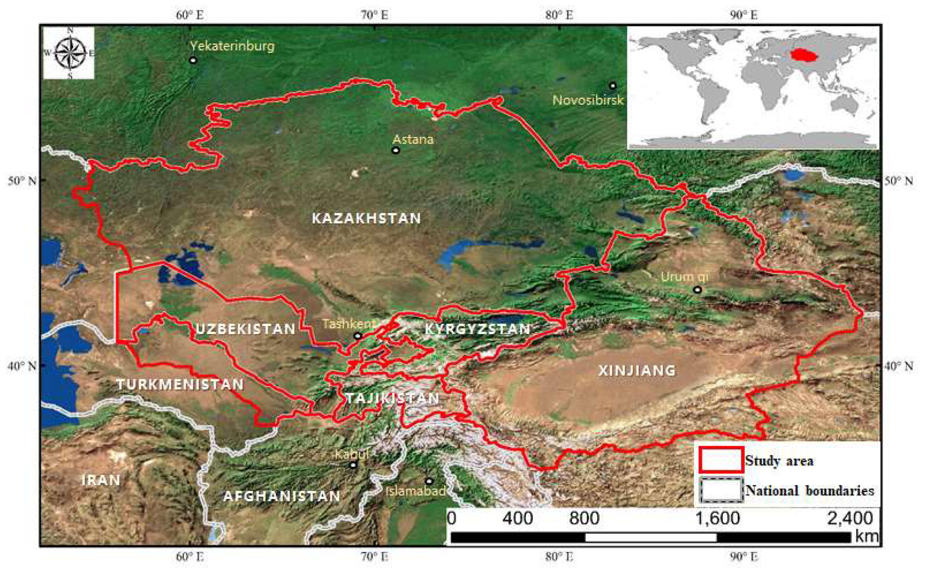
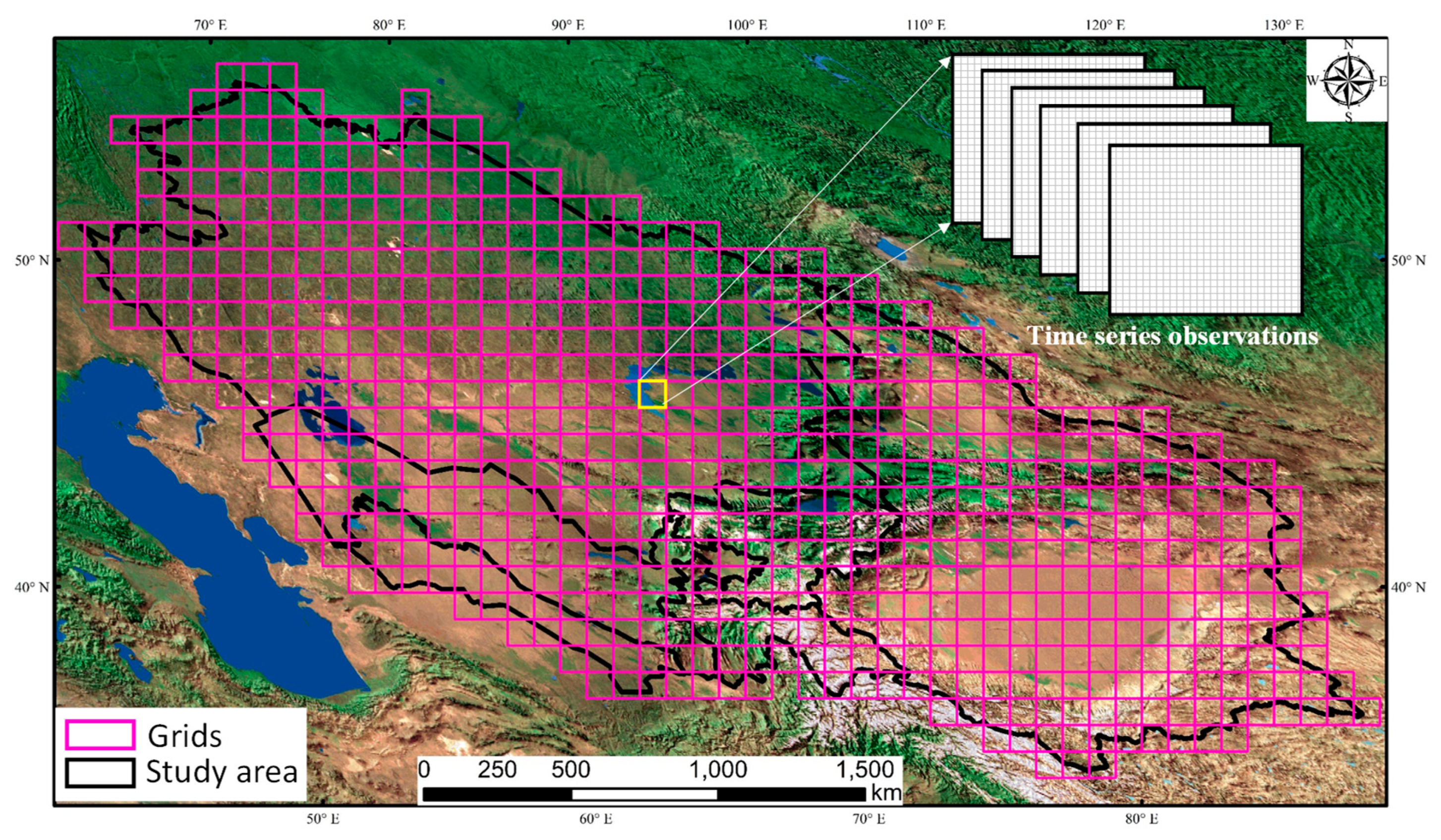
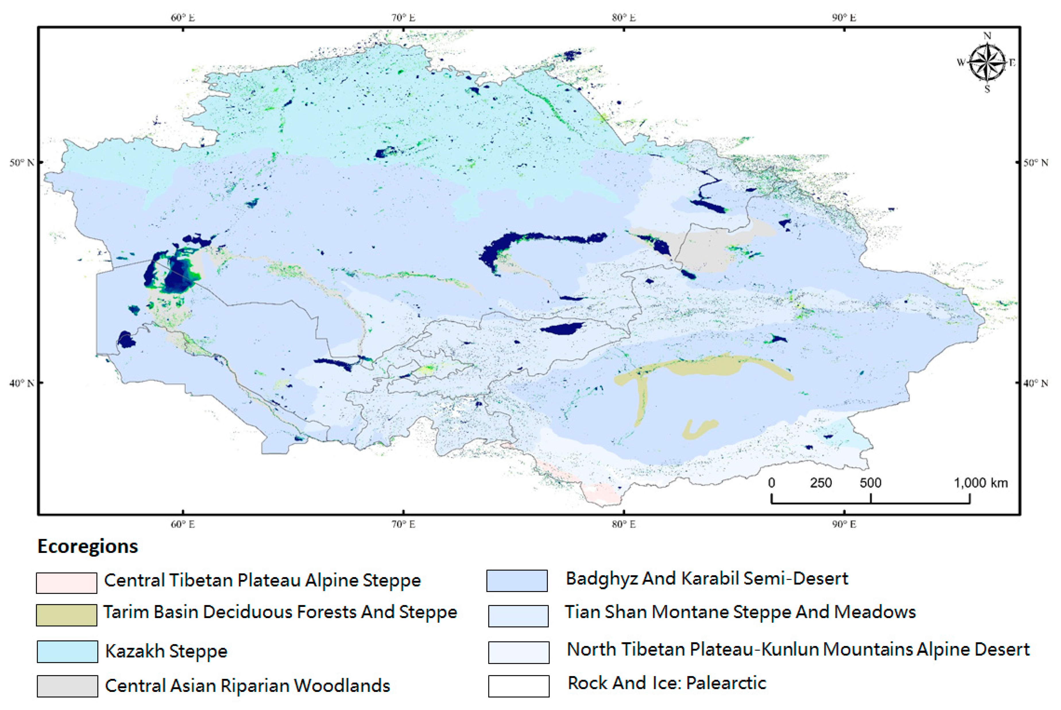
2.1. Study Area
2.2. Datasets
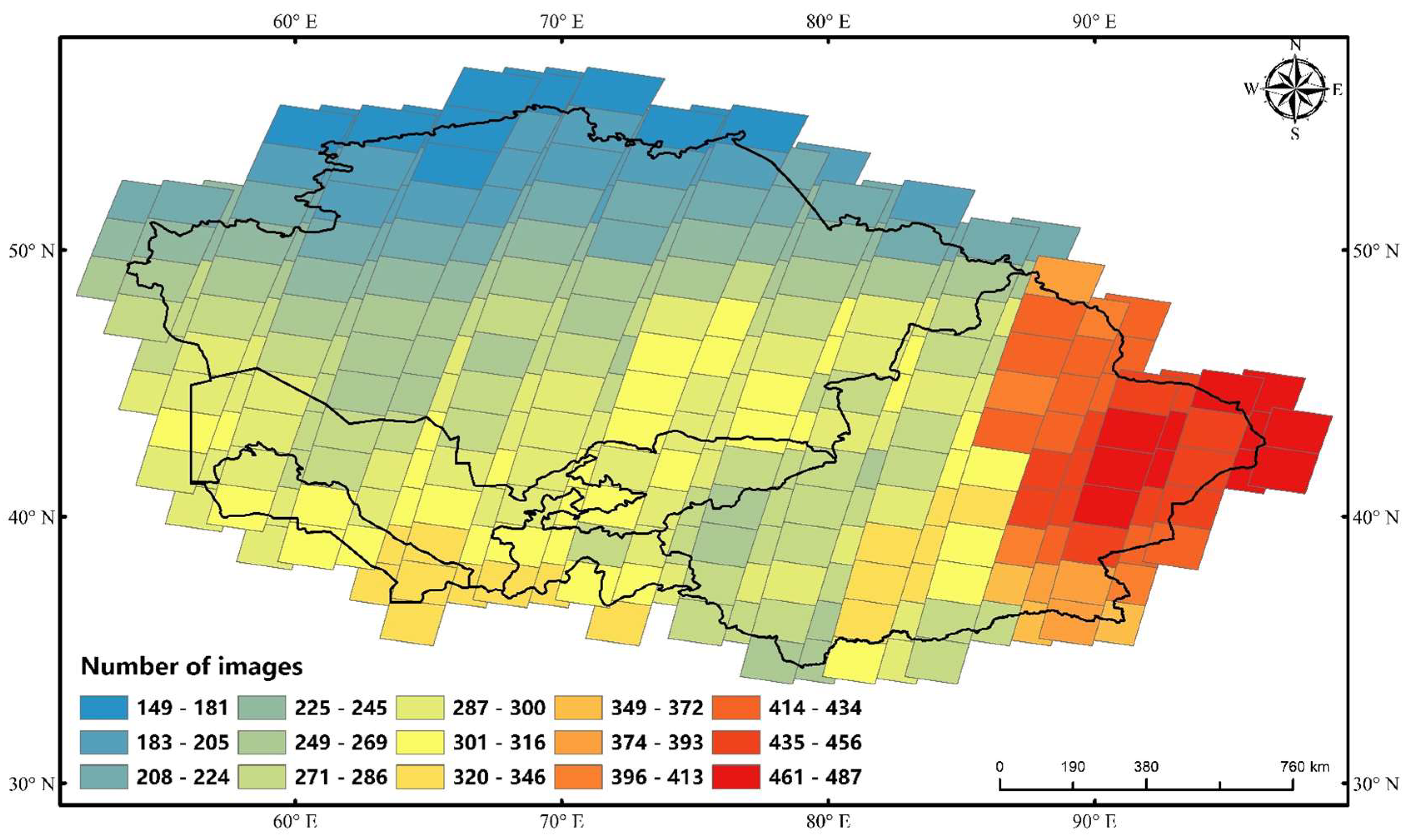
2.2.1. Landsat Data
2.2.2. Ancillary Datasets
2.3. Methods
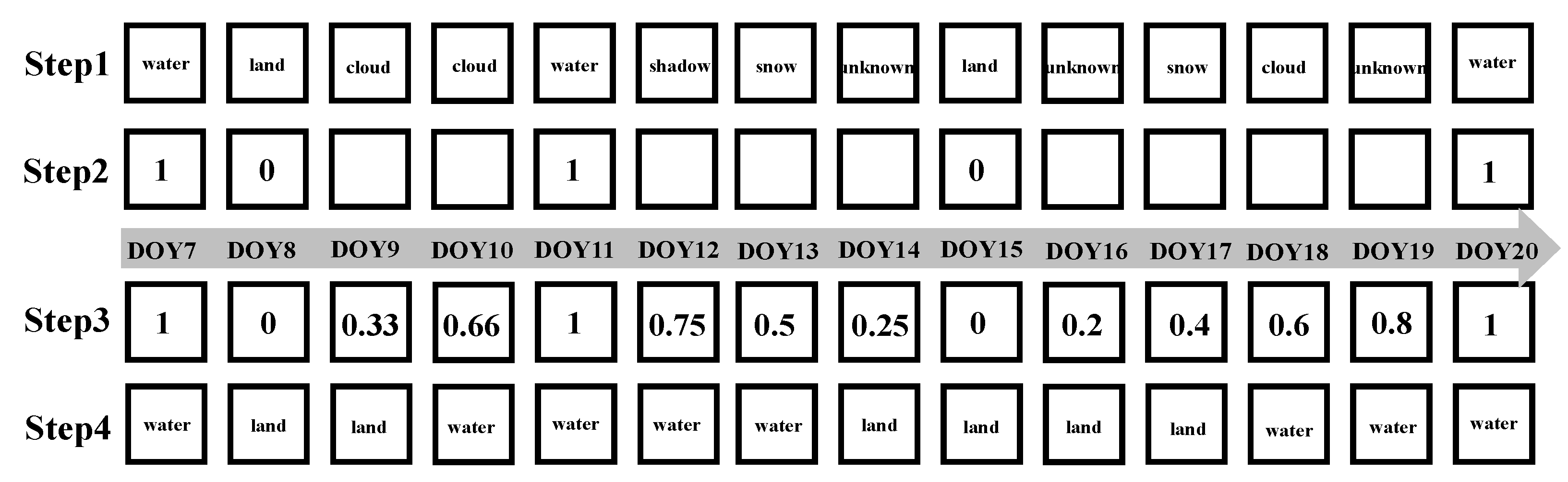
2.3.1. Water Detection Algorithm
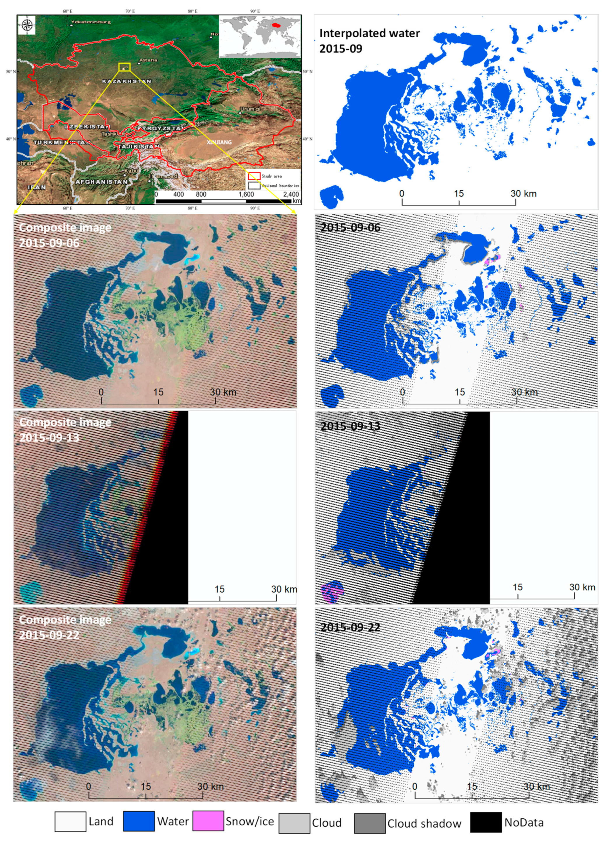
2.3.2. Temporal Interpolation
2.3.3. Implementation and Data Processing
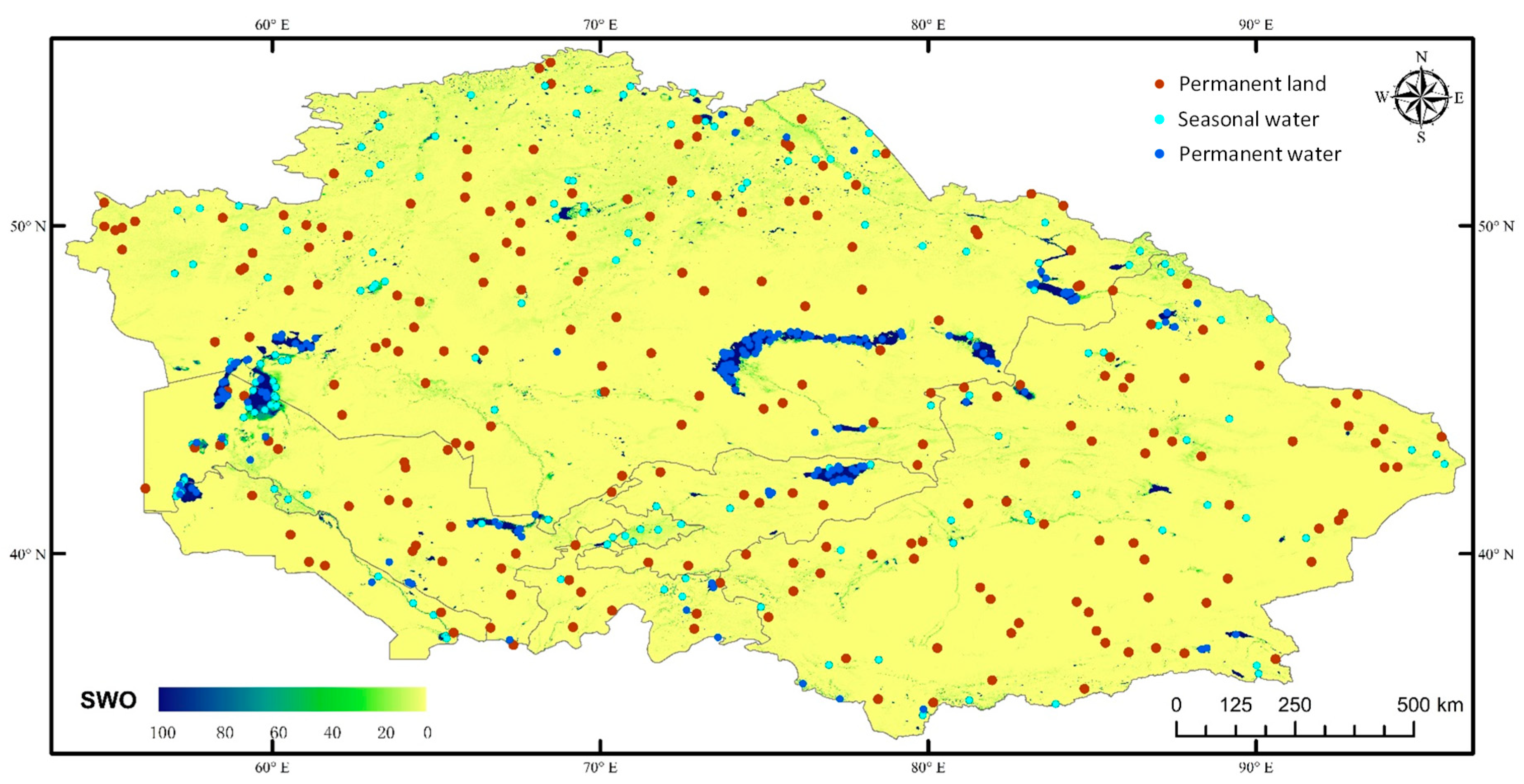
2.3.4. Accuracy Assessment
3. Results
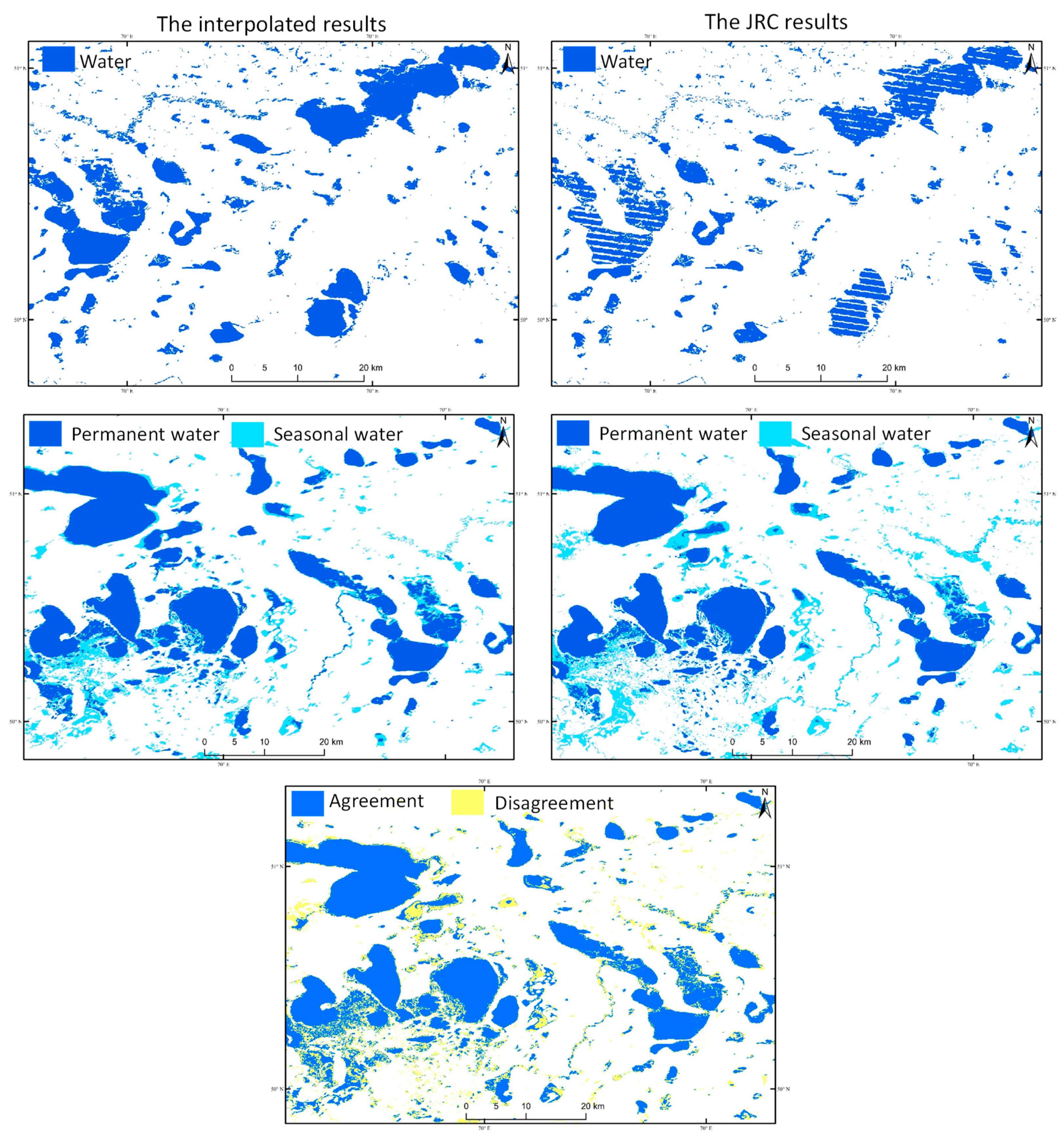
3.1. Surface Water Estimates and Its Uncertainties
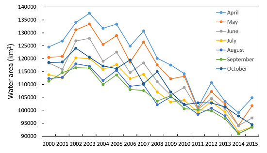
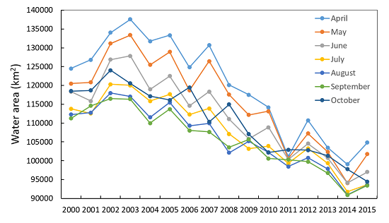
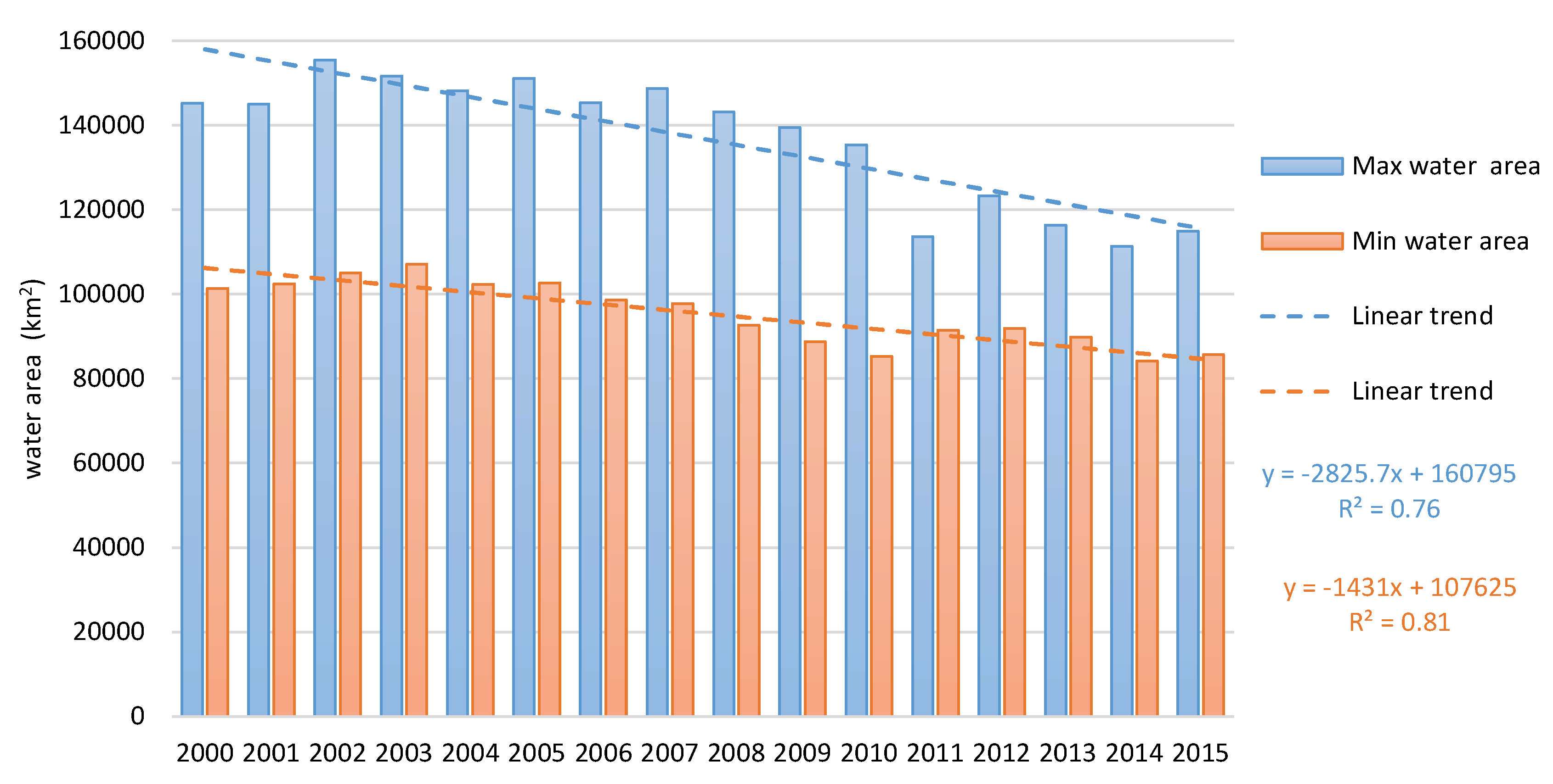
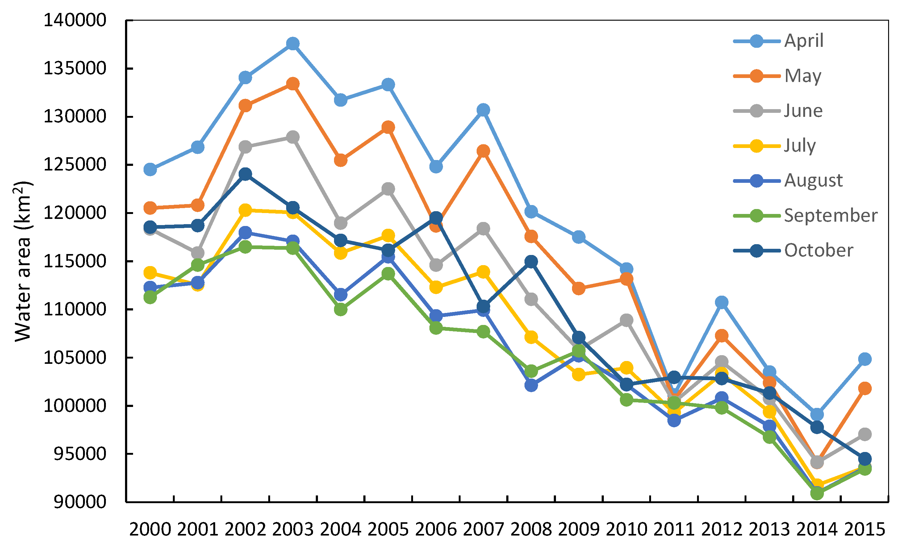
3.2. Surface Water Dynamics in the Area
4. Discussion
5. Conclusions
Author Contributions
Funding
Acknowledgments
Conflicts of Interest
References
- Feng, M.; Sexton, J.O.; Channan, S.; Townshend, J.R. A global, high-resolution (30-m) inland water body dataset for 2000: First results of a topographical-spectral classification algorithm. Int. J. Digit. Earth 2016, 9, 113–133. [Google Scholar] [CrossRef]
- Palmer, S.C.J.; Kutser, T.; Hunter, P.D. Remote sensing of inland waters: Challenges, progress and future directions. Remote Sens. Environ. 2015, 157, 1–8. [Google Scholar] [CrossRef] [Green Version]
- Bai, J.; Chen, X.; Li, J.; Yang, L.; Fang, H. Changes in the area of inland lakes in arid regions of central Asia during the past 30 years. Environ. Monit. Assess. 2011, 178, 247–256. [Google Scholar] [CrossRef] [PubMed]
- Yao, T. The response of environmental changes on Tibetan Plateau to global changes and adaptation strategy. Adv. Earth Sci. 2006, 21, 459–464. [Google Scholar]
- Li, C.; Kang, S. Review of studies in climate change over the Tibetan Plateau. Acta Geogr. Sin. Chin. Ed. 2006, 61, 335. [Google Scholar]
- Kang, S.; Xu, Y.; You, Q.; Flügel, W.A.; Pepin, N.; Yao, T. Review of climate and cryospheric change in the Tibetan Plateau. Environ. Res. Lett. 2010, 5, 015101. [Google Scholar] [CrossRef]
- Haas, E.M.; Bartholomé, E.; Combal, B. Time series analysis of optical remote sensing data for the mapping of temporary surface water bodies in sub-Saharan western Africa. J. Hydrol. 2009, 370, 52–63. [Google Scholar] [CrossRef]
- Kuenzer, C.; Guo, H.; Huth, J.; Leinenkugel, P.; Li, X.; Dech, S. Flood Mapping and Flood Dynamics of the Mekong Delta: ENVISAT-ASAR-WSM Based Time Series Analyses. Remote Sens. 2013, 5, 687–715. [Google Scholar] [CrossRef] [Green Version]
- Kuenzer, C.; Klein, I.; Ullmann, T.; Georgiou, E.; Baumhauer, R.; Dech, S. Remote sensing of river delta inundation: Exploiting the potential of coarse spatial resolution, temporally-dense MODIS time series. Remote Sens. 2015, 7, 8516–8542. [Google Scholar] [CrossRef]
- Feng, L.; Hu, C.; Chen, X.; Song, Q. Influence of the three gorges dam on total suspended matters in the Yangtze estuary and its adjacent coastal waters: Observations from MODIS. Remote Sens. Environ. 2014, 140, 779–788. [Google Scholar] [CrossRef]
- Ogilvie, A.; Belaud, G.; Delenne, C.; Bailly, J.S.; Bader, J.C.; Oleksiak, A.; Ferry, L.; Martin, D. Decadal monitoring of the Niger Inner Delta flood dynamics using MODIS optical data. J. Hydrol. 2015, 523, 368–383. [Google Scholar] [CrossRef] [Green Version]
- Klein, I.; Dietz, A.J.; Gessner, U.; Galayeva, A.; Myrzakhmetov, A.; Kuenzer, C. Evaluation of seasonal water body extents in Central Asia over the past 27 years derived from medium-resolution remote sensing data. Int. J. Appl. Earth Obs. Geoinf. 2014, 26, 335–349. [Google Scholar] [CrossRef]
- Sun, F.; Zhao, Y.; Gong, P.; Ma, R.; Dai, Y. Monitoring dynamic changes of global land cover types: Fluctuations of major lakes in China every 8 days during 2000–2010. Chin. Sci. Bull. 2014, 59, 171–189. [Google Scholar] [CrossRef]
- Yamazaki, D.; Trigg, M.A.; Ikeshima, D. Development of a global~ 90 m water body map using multi-temporal Landsat images. Remote Sens. Environ. 2015, 171, 337–351. [Google Scholar] [CrossRef]
- Global Land Survey (GLS). Available online: https://www.usgs.gov/land-resources/nli/landsat/global-land-survey-gls?qt-science_support_page_related_con=0#qt-science_support_page_related_con (accessed on 31 May 2019).
- Tulbure, M.G.; Broich, M.; Stehman, S.V.; Kommareddy, A. Surface water extent dynamics from three decades of seasonally continuous Landsat time series at subcontinental scale in a semi-arid region. Remote Sens. Environ. 2016, 178, 142–157. [Google Scholar] [CrossRef]
- Mueller, N.; Lewis, A.; Roberts, D.; Ring, S.; Melrose, R.; Sixsmith, J.; Lymburner, L.; McIntyre, A.; Tan, P.; Curnow, S. Water observations from space: Mapping surface water from 25 years of Landsat imagery across Australia. Remote Sens. Environ. 2016, 174, 341–352. [Google Scholar] [CrossRef]
- Halabisky, M.; Moskal, L.M.; Gillespie, A.; Hannam, M. Reconstructing semi-arid wetland surface water dynamics through spectral mixture analysis of a time series of Landsat satellite images (1984–2011). Remote Sens. Environ. 2016, 177, 171–183. [Google Scholar] [CrossRef]
- Pekel, J.-F.; Cottam, A.; Gorelick, N.; Belward, A.S. High-resolution mapping of global surface water and its long-term changes. Nature 2016, 540, 418. [Google Scholar] [CrossRef] [PubMed]
- Yan, Q.; Liao, J.; Sheng, G. Remote sensing analysis and hydrological model simulation of the variation of Ulan Ula lake in recent 40 years. Remote Sens. Land Res. 2014, 1, 152–157. [Google Scholar]
- Bai, J.; Chen, X.; Li, J.; Yang, L. Changes of inland lake area in arid Central Asia during 1975–2007: A remote-sensing analysis. J. Lake Sci. 2011, 1, 80–88. [Google Scholar]
- Chen, C.; Fu, W.; Hu, Z.; Li, X. Changes of main lakes in central Asia in recent 30 years based on remote sensing technology. Remote Sens. Land Res. 2015, 1, 146–152. [Google Scholar]
- Wu, J.; Ma, L.; JI, L. Lake surface change of the Aral Sea and its environmental effects in the arid region of the Central Asia. Arid Land Geogr. 2009, 3, 418–422. [Google Scholar]
- Li, J.; Chen, X.; Bao, A. Spatial-temporal characteristics of lake level changes in Central Asia during 2003-2009. J. Geogr. Sci. 2011, 66, 1219–1229. [Google Scholar]
- De Pauw, E. ICARDA regional GIS datasets for Central Asia: Explanatory notes. GIS unit technical bulletin. Int. Cent. Agric. Res. Dry Areas (ICARDA) 2008. Available online: http://gu.icarda.org/geocms/public/en/cms/metadata/index/133/Central+Asia%3A+Climate+Productivity+Index+%28Crop+Group+II%2C+rainfed%29%2E/ (accessed on 31 May 2019).
- Aizen, V.B.; Aizen, E.M.; Kuzmichenok, V.A. Geo-informational simulation of possible changes in Central Asian water resources. Glob. Planet. Chang. 2007, 56, 341–358. [Google Scholar] [CrossRef]
- UNDP. Water Resources of Kazakhstan in the New Millennium. 2004. Available online: http://www.undp.kz/library_of_publications/files/2496-19223.pdf (accessed on 31 May 2019).
- USGS Landsat Mission. Available online: http://landsat.usgs.gov (accessed on 31 May 2019).
- Wulder, M.A.; White, J.C.; Loveland, T.R.; Woodcock, C.E.; Belward, A.S.; Cohen, W.B.; Fosnight, E.A.; Shaw, J.; Masek, J.G.; Roy, D.P. The global Landsat archive: Status, consolidation, and direction. Remote Sens. Environ. 2016, 185, 271–283. [Google Scholar] [CrossRef] [Green Version]
- Pekel, J.-F.; Vancutsem, C.; Bastin, L.; Clerici, M.; Vanbogaert, E.; Bartholomé, E.; Defourny, P. A near real-time water surface detection method based on HSV transformation of MODIS multi-spectral time series data. Remote Sens. Environ. 2014, 140, 704–716. [Google Scholar] [CrossRef] [Green Version]
- Masek, J.G.; Vermote, E.F.; Saleous, N.E.; Wolfe, R.; Hall, F.G.; Huemmrich, K.F.; Gao, F.; Kutler, J.; Lim, T.K. A Landsat surface reflectance dataset for North America, 1990–2000. IEEE Geosci. Remote Sens. Lett. 2006, 3, 68–72. [Google Scholar] [CrossRef]
- Schmidt, G.; Jenkerson, C.B.; Masek, J.; Vermote, E.; Gao, F. Landsat Ecosystem Disturbance Adaptive Processing System (LEDAPS) Algorithm Description; US Geological Survey: Sioux Falls, SD, USA, 2013.
- Claverie, M.; Ju, J.; Masek, J.G.; Dungan, J.L.; Vermote, E.F.; Roger, J.-C.; Skakun, S.V.; Justice, C. The Harmonized Landsat and Sentinel-2 surface reflectance data set. Remote Sens. Environ. 2018, 219, 145–161. [Google Scholar] [CrossRef]
- USGS. Guide P. Landsat 8 Surface Reflectance Code (LaSRC) Product. Available online: https://prd-wret.s3-us-west-2.amazonaws.com/assets/palladium/production/s3fs-public/atoms/files/LSDS-1368_%20L8_Surface-Reflectance-Code-LASRC-Product-Guide.pdf (accessed on 31 May 2019).
- Zhu, Z.; Woodcock, C.E. Object-based cloud and cloud shadow detection in Landsat imagery. Remote Sens. Environ. 2012, 118, 83–94. [Google Scholar] [CrossRef]
- Tachikawa, T.; Kaku, M.; Iwasaki, A.; Gesch, D.B.; Oimoen, M.J.; Zhang, Z.; Danielson, J.J.; Krieger, T.; Curtis, B.; Haase, J.; et al. ASTER Global Digital Elevation Model Version 2-Summary of Validation Results; NASA: Washington, DC, USA, 2011.
- Schaaf, C.B.; Gao, F.; Strahler, A.H.; Lucht, W.; Li, X.; Tsang, T.; Strugnell, N.C.; Zhang, X.; Jin, Y.; Muller, J.-P. First operational BRDF, albedo nadir reflectance products from MODIS. Remote Sens. Environ. 2002, 83, 135–148. [Google Scholar] [CrossRef] [Green Version]
- Carroll, M.; Townshend, J.R.; DiMiceli, C.M.; Noojipady, P.; Sohlberg, R.A. A new global raster water mask at 250 m resolution. Int. J. Digit. Earth 2009, 2, 291–308. [Google Scholar] [CrossRef]
- USGS. SRTM Water Body Dataset. 2012. Available online: https://www.usgs.gov/centers/eros/science/usgs-eros-archive-digital-elevation-shuttle-radar-topography-mission-water-body?qt-science_center_objects=0#qt-science_center_objects (accessed on 31 May 2019).
- MODIS Water Dataset (MOD44W). Available online: http://landcover.org/data/watermask (accessed on 31 May 2019).
- Google Earth Engine. Available online: https://developers.google.com/earth-engine (accessed on 31 May 2019).
- Quinlan, J.R. Induction of decision trees. Mach. Learn. 1986, 1, 81–106. [Google Scholar] [CrossRef] [Green Version]
- Roy, D.P.; Ju, J.; Kline, K.; Scaramuzza, P.L.; Kovalskyy, V.; Hansen, M.; Loveland, T.R.; Vermote, E.; Zhang, C. Web-enabled Landsat Data (WELD): Landsat ETM+ composited mosaics of the conterminous United States. Remote Sens. Environ. 2010, 114, 35–49. [Google Scholar] [CrossRef]
- Edwards, K. Geometric processing of digital images of the planets. Photogramm. Eng. Remote Sens. 1987, 53, 1219–1222. [Google Scholar]
- GDAL/OGR Open-Source Libraries. Available online: http://www.gdal.org/ (accessed on 31 May 2019).
- PROJ4 Open-Source Libraries. Available online: http://trac.osgeo.org/proj/ (accessed on 31 May 2019).
- NumPy Open-Source Libraries. Available online: http://www.numpy.org/ (accessed on 31 May 2019).
- SciPy Open-Source Libraries. Available online: http://www.scipy.org/ (accessed on 31 May 2019).
- Matplotlib Open-Source Libraries. Available online: http://matplotlib.org/ (accessed on 31 May 2019).
- Stehman, S.V. Sampling designs for accuracy assessment of land cover. Int. J. Remote Sens. 2009, 30, 5243–5272. [Google Scholar] [CrossRef]
- Ying, Q.; Hansen, M.C.; Potapov, P.V.; Tyukavina, A.; Wang, L.; Stehman, S.V.; Moore, R.; Hancher, M. Global bare ground gain from 2000 to 2012 using Landsat imagery. Remote Sens. Environ. 2017, 194, 161–176. [Google Scholar] [CrossRef] [Green Version]
- Olson, D.M.; Dinerstein, E.; Wikramanayake, E.D.; Burgess, N.D.; Powell, G.V.; Underwood, E.C.; D’amico, J.A.; Itoua, I.; Strand, H.E.; Morrison, J.C. Terrestrial ecoregions of the world: A new map of life on Earth: A new global map of terrestrial ecoregions provides an innovative tool for conserving biodiversity. BioScience 2001, 51, 933–938. [Google Scholar] [CrossRef]
- Foody, G.M.; Muslim, A.M.; Atkinson, P.M. Super-resolution mapping of the waterline from remotely sensed data. Int. J. Remote Sens. 2005, 26, 5381–5392. [Google Scholar] [CrossRef]
- Niroumand-Jadidi, M.; Vitti, A. Reconstruction of river boundaries at sub-pixel resolution: Estimation and spatial allocation of water fractions. ISPRS Int. J. Geo-Inf. 2017, 6, 383. [Google Scholar] [CrossRef]
- Li, L.; Chen, Y.; Xu, T.; Liu, R.; Shi, K.; Huang, C. Super-resolution mapping of wetland inundation from remote sensing imagery based on integration of back-propagation neural network and genetic algorithm. Remote Sens. Environ. 2015, 164, 142–154. [Google Scholar] [CrossRef]
- Messager, M.L.; Lehner, B.; Grill, G.; Nedeva, I.; Schmitt, O. Estimating the volume and age of water stored in global lakes using a geo-statistical approach. Nature Commun. 2016, 7, 13603. [Google Scholar] [CrossRef]


| Reference | ||||
|---|---|---|---|---|
| Water | Non-Water | UA | ||
| Map (Algorithm) | Water | 30.246 | 1.323 | 87.12 (± 3.21) |
| Non-water | 0.412 | 68.005 | 99.96 (± 0.04) | |
| PA | 98.24 (±1.02) | 99.15 (±0.59) | 99.59 (±0.32) | |
| Strata | Class | Spring | Summer | Autumn | Winter | |
|---|---|---|---|---|---|---|
| Permanent water N = 780 | OA | 99.03 (±0.02) | 100 (±0.00) | 99.52 (±0.02) | 99.01 (±0.03) | |
| UA | Water | 98.87 (±1.01) | 100 (±0.00) | 100 (±0.00) | 99.57 (±0.30) | |
| Non-water | 100 (±0.00) | 100 (±0.00) | 92.12 (±0.03) | 97.89 (±0.02) | ||
| PA | Water | 100 (±0.00) | 100 (±0.00) | 99.42 (±0.54) | 99.23 (±1.10) | |
| Non-water | 95.02 (±0.02) | 100 (±0.00) | 100 (±0.00) | 98.83 (±0.02) | ||
| Seasonal water N = 792 | OA | 92.92 (±0.13) | 93.67 (±0.11) | 90.11 (±0.11) | 85.36 (±0.19) | |
| UA | Water | 74.16 (±3.14) | 82.58 (±2.77) | 72.87 (±2.64) | 70.21 (±1.99) | |
| Non-water | 97.64 (±0.08) | 98.83 (±0.03) | 98.12 (±0.05) | 99.92 (±0.01) | ||
| PA | Water | 87.23 (±2.99) | 94.45 (±1.38) | 90.01 (±2.01) | 99.12 (±0.42) | |
| Non-water | 93.87 (±0.11) | 93.12 (±0.12) | 89.67 (±0.12) | 83.49 (±0.17) | ||
| Permanent land N = 784 | OA | 99.87 (± 0.36) | 99.99 (±0.02) | 99.59 (±0.82) | 98.78 (±3.56) | |
| UA | Water | 92.32 (±10.89) | 98.48 (±4.01) | 90.26 (±16.32) | 80.89 (±19.32) | |
| Non-water | 98.71 (±0.14) | 98.56 (±0.11) | 97.43 (±0.22) | 99.78 (±0.03) | ||
| PA | Water | 100 (±0.00) | 100 (±0.00) | 100 (±0.00) | 100 (±0.00) | |
| Non-water | 99.89 (±0.49) | 99.98 (±0.02) | 99.56 (±0.89) | 98.01 (±0.83) |
| Month | April | May | June | July | August | September | October |
|---|---|---|---|---|---|---|---|
| AC/Slope | −2317.39 | −2148.73 | −1957.20 | −1724.14 | −1631.15 | −1596.67 | −1828.94 |
| RC | −1.94 | −1.86 | −1.75 | −1.60 | −1.54 | −1.51 | −1.66 |
| R2 | 0.747 | 0.729 | 0.794 | 0.814 | 0.856 | 0.889 | 0.880 |
© 2019 by the authors. Licensee MDPI, Basel, Switzerland. This article is an open access article distributed under the terms and conditions of the Creative Commons Attribution (CC BY) license (http://creativecommons.org/licenses/by/4.0/).
Share and Cite
Che, X.; Feng, M.; Sexton, J.; Channan, S.; Sun, Q.; Ying, Q.; Liu, J.; Wang, Y. Landsat-Based Estimation of Seasonal Water Cover and Change in Arid and Semi-Arid Central Asia (2000–2015). Remote Sens. 2019, 11, 1323. https://doi.org/10.3390/rs11111323
Che X, Feng M, Sexton J, Channan S, Sun Q, Ying Q, Liu J, Wang Y. Landsat-Based Estimation of Seasonal Water Cover and Change in Arid and Semi-Arid Central Asia (2000–2015). Remote Sensing. 2019; 11(11):1323. https://doi.org/10.3390/rs11111323
Chicago/Turabian StyleChe, Xianghong, Min Feng, Joe Sexton, Saurabh Channan, Qing Sun, Qing Ying, Jiping Liu, and Yong Wang. 2019. "Landsat-Based Estimation of Seasonal Water Cover and Change in Arid and Semi-Arid Central Asia (2000–2015)" Remote Sensing 11, no. 11: 1323. https://doi.org/10.3390/rs11111323